Dynamics of an Eco-Epidemic Predator–Prey Model Involving Fractional Derivatives with Power-Law and Mittag–Leffler Kernel

Abstract

In this paper, we consider a fractional-order eco-epidemic model based on the Rosenzweig–MacArthur predator–prey model. The model is derived by assuming that the prey may be infected by a disease. In order to take the memory effect into account, we apply two fractional differential operators, namely the Caputo fractional derivative (operator with power-law kernel) and the Atangana–Baleanu fractional derivative in the Caputo (ABC) sense (operator with Mittag–Leffler kernel). We take the same order of the fractional derivative in all equations for both senses to maintain the symmetry aspect. The existence and uniqueness of solutions of both eco-epidemic models (i.e., in the Caputo sense and in ABC sense) are established. Both models have the same equilibrium points, namely the trivial (origin) equilibrium point, the extinction of infected prey and predator point, the infected prey free point, the predator-free point and the co-existence point. For a model in the Caputo sense, we also show the non-negativity and boundedness of solution, perform the local and global stability analysis and establish the conditions for the existence of Hopf bifurcation. It is found that the trivial equilibrium point is a saddle point while other equilibrium points are conditionally asymptotically stable. The numerical simulations show that the solutions of the model in the Caputo sense strongly agree with analytical results. Furthermore, it is indicated numerically that the model in the ABC sense has quite similar dynamics as the model in the Caputo sense. The essential difference between the two models is the convergence rate to reach the stable equilibrium point. When a Hopf bifurcation occurs, the bifurcation points and the diameter of the limit cycles of both models are different. Moreover, we also observe a bistability phenomenon which disappears via Hopf bifurcation.

1. Introduction

The long history of mathematical biology reveals that predator–prey modeling plays an imperative role in scientific research. Since the classical Lotka–Volterra, as the fundamental predator–prey model, have been proposed [1,2,3], the theoretical ecology has been constantly developed. The Lotka–Volterra model has been modified by a lot of researchers to contrive the relevant model which corresponds to the actual phenomena, such as the functional response [4,5,6,7,8,9], the Allee effect [10,11,12,13,14], the impact of competition [15,16,17] and so forth. All of these modifications affect the density of populations as the result of interactions between two or more populations. From the biological point of view, the population density also depends on the epidemiological frameworks, which leads to the increment of the death rate caused by the disease in the population. Eco-epidemiology describes the occurrence of ecological and epidemiological circumstances simultaneously [18,19,20,21,22,23]. For instance, in a biotope that involves pests and its natural enemies, we observe that the eco-epidemiological problem occurs and described by the interaction between pest and its predator. One or both populations may be infected by a disease caused by microbiological pathogens such as parasites, viruses, fungi and bacteria, for further see refs. [24,25,26,27,28] and some references therein. For the real-world example, to suppress the growth rate of rats (Rattus sp.) in agricultural landscape, the farmers use barn owls (tyto alba) and some pathogens such as viruses (paramyxoviridae and pneumovirus family), bacterias (klebsiella pneumoniae, mycoplasma pulmonis, citrobacter rodentium and streptococcus pneumoniae), and parasites (giardia muris, spironucleus muris, oxyuriasis and acariasis) [29,30,31,32,33].

Regarding to the description above, some researchers have successfully constructed and studied the eco-epidemiological problem in a deterministic model. Mondal et al. [21], Wang et al. [34] and Suryanto et al. [35] study the dynamics of the interaction between two populations in a predator–prey relationship where the prey is infected by a disease and the predator is hunting the infected prey. In facts, many natural phenomena in the ecological system show that predation still occurs although the infected prey does not exist. This means both susceptible and infected prey are regarded to be predated. Based on this assumption, Sahoo [19], Saifuddin et al. [20], Panigoro et al. [23], Upadhyay et al. [36] and Nugraheni et al. [37] study the eco-epidemic model with the predation existing on both susceptible and infected prey. The fundamental differences of their models lie on the infectious transmission behavior, the predator functional response, the existence of the Allee effect and the operator of the derivative. Here, we study the eco-epidemic model formulated under the following assumptions.

(a)

In the presence of disease, the prey is divided into two compartments, namely susceptible prey $S\left(t\right)$ and infected prey $I\left(t\right)$. The susceptible prey becomes infected when the individuals have contact with the infected prey. Since the density of prey and predator are assumed large enough, the infection rate due to this contact is bilinear which is symbolized by b.

(b)

In the presence of the predator–prey relationship, the interaction between susceptible prey, infected prey and predator is following the Rosenzweig–MacArthur model [38] with a few adjustments. The susceptible prey growth logistically with intrinsic growth rate r and environmental carrying capacity K. The infected prey competes for food with the susceptible prey but has no contribution to the growth rate of susceptible prey. Both susceptible prey and infected prey are predated following Holling type-II with the attack rate of predator on susceptible prey $m_s$, the attack rate of predator on infected prey $m_i$, the half-saturation constant of predator for susceptible prey $k_s$ and the half-saturation constant of predator for infected prey $k_i$. Since both predations contribute to the predator birth, the conversion efficiency consists of two parts, i.e., the conversion efficiency of predator on susceptible prey $b_s$ and the conversion efficiency of predator on infected prey $b_i$. It is also assumed that both infected prey and predator are reduced due to mortality following exponential decay where d is the death rate of infected prey, and a is the death rate of predator.

Based on above assumptions, we have the following eco-pidemic model.

$$\begin{array}{cc}\hfill \frac{dS}{dt}=& rS\left(1-\frac{S+I}{K}\right)-bSI-\frac{m_{s}SP}{k_s+S},\hfill \\ \hfill \frac{dI}{dt}=& bSI-dI-\frac{m_{i}IP}{k_i+I},\hfill \\ \hfill \frac{dP}{dt}=& \left(\frac{b_{s}S}{k_s+S}+\frac{b_{i}I}{k_i+I}-a\right)P,\hfill \end{array}$$

(1)

For simplicity, model (1) is transformed into a non-dimensional system by introducing transformation of variables $(S,I,P,t)\to \left(\frac{S}{K},\frac{I}{K},\frac{m_{s}P}{rK},rt\right)$ to obtain the following eco-epidemic model.

$$\begin{array}{cc}\hfill \frac{dS}{dt}=& \left[1-S-(1+\widehat{\eta })I-\frac{P}{\kappa +S}\right]S,\hfill \\ \hfill \frac{dI}{dt}=& \left[\widehat{\eta }S-\widehat{\delta }-\frac{\widehat{m}P}{\omega +I}\right]I,\hfill \\ \hfill \frac{dP}{dt}=& \left[\frac{\widehat{\mu }S}{\kappa +S}+\frac{\widehat{\beta }I}{\omega +I}-\widehat{q}\right]P,\hfill \end{array}$$

(2)

where $\widehat{\eta }=\frac{bK}{r}$, $\widehat{\delta }=\frac{d}{r}$, $\widehat{m}=\frac{m_i}{m_s}$, $\widehat{\mu }=\frac{b_s}{r}$, $\widehat{\beta }=\frac{b_i}{r}$, $\kappa =\frac{k_s}{K}$, $\omega =\frac{k_i}{K}$ and $\widehat{q}=\frac{a}{r}$.

To approach the superlative shape of the eco-epidemiological model, the ordinary calculus is considered less effective in describing the complex ecological phenomena that involves the system memory and hereditary biological properties of complex multiple timescale dynamics, see refs. [39,40,41]. To overcome such problem, many researchers apply fractional calculus because it is considered to have the ability to represent biological conditions related to the memory effects more powerfully and accurately than the classical calculus [42,43,44,45,46,47,48]. Particularly, the fractional-order derivatives, as part of the fundamental theory of fractional calculus, have nonlocal properties which are naturally connected to the biological systems. It means that the current state of population density depends on all earlier states [49,50,51]. If we revisited the evolution of fractional-order derivative, the Riemann–Liouville [52] and Caputo [53] operators have been widely applied to the biological modeling. To investigate the behavior of the fractional-order dynamical system, the theoretical aspect of the Caputo operator is the most complete tool compared to others, see refs. [52,54,55]. However, the kernels of the first two definitions of fractional operators are single and local [56,57,58,59]. Therefore, Caputo operator is not sufficient enough to express better nonlocal dynamics. To cover the limitation of Caputo operator, in 2015, Caputo and Fabrizio proposed a new fractional operator, which is called the Caputo–Fabrizio derivative [60]. The non-singular and exponential kernel of this fractional derivative is the novelty of their result and has been successfully applied in several fields [40,61,62,63]. One year later, Atangana and Baleanu introduced a new fractional operator with a nonlocal and non-singular kernel. Such an operator is well-known as the Atangana–Baleanu operator, which has all the advantages of the Caputo–Fabrizio operator but it uses the Mittag–Leffler function as its kernel [64]. Most researchers reveal that the Atangana–Baleanu operator gives better results and claim that the effect of memory is represented efficiently, see refs. [9,40,51,65].

For a better approach in epidemiological modeling, the fractional-order derivative is utilized in a similar way with [48,66] which replace the first-order derivative $\frac{d}{dt}$ at the left-hand side of model (2) with the fractional-order derivative ${\mathcal{D}}_t^{\alpha }$. Therefore, we obtain

$$\begin{array}{cc}\hfill {\mathcal{D}}_t^{\alpha }S=& \left[1-S-(1+\widehat{\eta })I-\frac{P}{\kappa +S}\right]S,\hfill \\ \hfill {\mathcal{D}}_t^{\alpha }I=& \left[\widehat{\eta }S-\widehat{\delta }-\frac{\widehat{m}P}{\omega +I}\right]I,\hfill \\ \hfill {\mathcal{D}}_t^{\alpha }P=& \left[\frac{\widehat{\mu }S}{\kappa +S}+\frac{\widehat{\beta }I}{\omega +I}-\widehat{q}\right]P.\hfill \end{array}$$

(3)

Pay close attention to the dimension of the equations in model (3), where the fractional-order derivatives have the dimensions of (time)${}^{-\alpha }$ while the parameters $\widehat{\eta },\widehat{\delta },\widehat{m},\widehat{\mu },\widehat{\beta }$ and $\widehat{q}$ have the dimensions of (time)${}^{-1}$. This circumstance means the inconsistency of physical dimensions in the model (3) and can be surmounted by rescaling the parameters as in the following model.

$$\begin{array}{cc}\hfill {\mathcal{D}}_t^{\alpha }S=& \left[1-S-(1+{\widehat{\eta }}^{\alpha })I-\frac{P}{\kappa +S}\right]S,\hfill \\ \hfill {\mathcal{D}}_t^{\alpha }I=& \left[{\widehat{\eta }}^{\alpha }S-{\widehat{\delta }}^{\alpha }-\frac{{\widehat{m}}^{\alpha }P}{\omega +I}\right]I,\hfill \\ \hfill {\mathcal{D}}_t^{\alpha }P=& \left[\frac{{\widehat{\mu }}^{\alpha }S}{\kappa +S}+\frac{{\widehat{\beta }}^{\alpha }I}{\omega +I}-{\widehat{q}}^{\alpha }\right]P.\hfill \end{array}$$

(4)

By applying new parameters $\widehat{\eta }=\eta$, $\widehat{\delta }=\delta$, $\widehat{m}=m$, $\widehat{\mu }=\mu$, $\widehat{\beta }=\beta$ and $\widehat{q}=q$, we achieve

$$\begin{array}{cc}\hfill {\mathcal{D}}_t^{\alpha }S=& \left[1-S-(1+\eta )I-\frac{P}{\kappa +S}\right]S,\hfill \\ \hfill {\mathcal{D}}_t^{\alpha }I=& \left[\eta S-\delta -\frac{mP}{\omega +I}\right]I,\hfill \\ \hfill {\mathcal{D}}_t^{\alpha }P=& \left[\frac{\mu S}{\kappa +S}+\frac{\beta I}{\omega +I}-q\right]P.\hfill \end{array}$$

(5)

We note that model (5) consists of three fractional differential equations. The order of the fractional derivative in all equations is set to be the same to maintain their symmetrical aspect.

Notice that we have to assume in model (5) that the disease transmission follows a bilinear incidence rate. Previously, Nugraheni et al. [37] have studied the same model but with saturated incidence rate. However, Nugraheni et al. [37] have only presented some numerical simulations of model (5) with Caputo sense without any analytical studies. In this article, we start our work by constructing the fractional-order eco-epidemic model consisting of the model assumptions, the first-order modeling, its non-dimensional form and the fractional-order modeling including the replacement of the first-order derivative with fractional-order derivative and the time dimension adjustment for some parameters to prevent the inconsistency of physical dimensions. Furthermore, we present the complete dynamics of model (5) with Caputo operator including the local and global stability, the existence of Hopf bifurcation and their appropriated numerical simulations. We also use the Atangana–Baleanu in Caputo sense as the fractional-order operator of model (5) numerically by previously showing the existence and uniqueness of solution of the model. We compare numerically the difference between model (5) with Caputo and Atangana–Baleanu operators, especially the difference of the dynamical behaviors when the Hopf bifurcation occurs. All of these analytical results and numerical simulations have never been done in [37], which is the novelty of our work.

This paper is organized as follows. In Section 2, we present some fundamental concepts which consist of definitions, theorems and lemmas that are associated with Caputo and Atangana–Baleanu derivatives and dynamical systems. Further, in Section 3, we investigate the dynamics of model (5) with Caputo derivative. The investigation includes the existence, uniqueness, non-negativity, boundedness of the solutions, the existence of equilibrium points, their local and global stability, as well as the occurrence of Hopf bifurcation. The existence and uniqueness of solutions of model (5) with Atangana–Baleanu derivative in Caputo sense are discussed in Section 4. To support our theoretical findings, we demonstrate some numerical simulations in Section 5. Finally, we present some conclusions in Section 6.

2. Fundamental Concepts

In this section, we present the important results from previous research such as definitions, theorems and lemmas associated with the fractional-order differential equation.

Definition 1

([55]). Suppose $0<\alpha \le 1$. The Caputo fractional derivative of order$-\alpha$ is defined by

$${}^C{\mathcal{D}}_t^{\alpha }f\left(t\right)=\frac{1}{\Gamma (1-\alpha )}{\int }_0^t{(t-s)}^{-\alpha }{f}^{\prime }\left(s\right)ds,$$

(6)

where $t\ge 0,$$f\in C^n([0,+\infty ),\mathbb{R})$, and Γ is the Gamma function.

Definition 2

([64]). Suppose $0<\alpha \le 1$. The Atangana–Baleanu fractional integral and derivative in Caputo sense of order$-\alpha$ (ABC sense) are respectively defined by

$$\begin{array}{cc}\hfill {}^{ABC}{\mathcal{I}}_t^{\alpha }f\left(t\right)=& \frac{1-\alpha }{B\left(\alpha \right)}f\left(t\right)+\frac{\alpha }{\Gamma \left(\alpha \right)B\left(\alpha \right)}{\int }_0^t{(t-s)}^{\alpha -1}f\left(s\right)ds,\hfill \\ \hfill {}^{ABC}{\mathcal{D}}_t^{\alpha }f\left(t\right)=& \frac{B\left(\alpha \right)}{1-\alpha }{\int }_0^t{E}_{\alpha }\left[-\frac{\alpha }{1-\alpha }{(t-s)}^{\alpha }\right]f^{\prime }\left(s\right)ds,\hfill \end{array}$$

where $t\ge 0,$ $f\in C^n([0,+\infty ),\mathbb{R})$, $E_{\alpha }$ is the Mittag–Leffler function defined by $E_{\alpha }\left(t\right)={\sum }_{k=0}^{\infty }\frac{t^k}{\Gamma (\alpha k+1)}$, and $B\left(\alpha \right)$ is a normalization function with $B\left(0\right)=B\left(1\right)=1$. In this paper, we define $B\left(\alpha \right)=1-\alpha +\frac{\alpha }{\Gamma \left(\alpha \right)}$.

Theorem 1

([64]). By using the inverse Laplace transform and convolution theorem, the unique solution of the time fractional differential equation

$${}^{ABC}{\mathcal{D}}_t^{\alpha }f\left(t\right)=\phi \left(t\right)$$

(7)

can be written as

$$f\left(t\right)=\frac{1-\alpha }{B\left(\alpha \right)}\phi \left(t\right)+\frac{\alpha }{\Gamma \left(\alpha \right)B\left(\alpha \right)}{\int }_0^t\phi \left(s\right){(t-s)}^{\alpha -1}ds.$$

(8)

Lemma 1

([67]). Let $0<\alpha \le 1$. Suppose that $f\left(t\right)\in C[a,b]$ and ${}^C{\mathcal{D}}_t^{\alpha }f\left(t\right)\in C[a,b]$. If ${}^C{\mathcal{D}}_t^{\alpha }f\left(t\right)\ge 0,\forall t\in (a,b)$, then $f\left(t\right)$ is a non-decreasing function for each $t\in [a,b]$. If ${}^C{\mathcal{D}}_t^{\alpha }f\left(t\right)\le 0,\forall t\in (a,b)$, then $f\left(t\right)$ is a non-increasing function for each $t\in [a,b]$.

Theorem 2

(Matignon condition [55,68]). Consider a Caputo fractional-order system

$${}^C{\mathcal{D}}_t^{\alpha }\overrightarrow{x}=\overrightarrow{f}\left(\overrightarrow{x}\right);\overrightarrow{x}\left(0\right)={\overrightarrow{x}}_0;\alpha \in (0,1].$$

(9)

A point ${\overrightarrow{x}}^{*}$ is called an equilibrium point of Equation (9) if it satisfies $\overrightarrow{f}\left({\overrightarrow{x}}^{*}\right)=0$. This equilibrium point is locally asymptotically stable if all eigenvalues ${\lambda }_j$ of the Jacobian matrix $J=\frac{\partial \overrightarrow{f}}{\partial \overrightarrow{x}}$ evaluated at ${\overrightarrow{x}}^{*}$ satisfy $|arg\left({\lambda }_j\right)|>\frac{\alpha \pi }{2}$. If there exists at least one eigenvalue that satisfies $|arg\left({\lambda }_k\right)|>\frac{\alpha \pi }{2}$ while $|arg\left({\lambda }_l\right)|<\frac{\alpha \pi }{2}$, $k\ne l$, then ${\overrightarrow{x}}^{*}$ is a saddle-point.

Lemma 2

([69]). Consider a Caputo fractional-order system

$${}^C{\mathcal{D}}_t^{\alpha }x\left(t\right)=f(t,x\left(t\right)),t>0,x\left(0\right)\ge 0,\alpha \in (0,1],$$

(10)

where $f:(0,\infty )\times \Omega \to {\mathbb{R}}^n,\Omega \subseteq {\mathbb{R}}^n$. A unique solution of Equation (10) on $(0,\infty )\times \Omega$ exists if $f(t,x(t\left)\right)$ satisfies the locally Lipschitz condition with respect to x.

Lemma 3

(Standard comparison theorem for Caputo fractional-order derivative [42]). Let $x\left(t\right)\in C\left([0,+\infty )\right)$. If $x\left(t\right)$ satisfies

$${}^C{\mathcal{D}}_t^{\alpha }x\left(t\right)+\lambda x\left(t\right)\le \mu ,x\left(0\right)=x_0,$$

where $\alpha \in (0,1],(\lambda ,\mu )\in {\mathbb{R}}^2$ and $\lambda \ne 0$, then

$$x\left(t\right)\le \left(x_0-\frac{\mu }{\lambda }\right)E_{\alpha }[-\lambda t^{\alpha }]+\frac{\mu }{\lambda }.$$

Lemma 4

([70]). Let $x\left(t\right)\in C\left({\mathbb{R}}_{+}\right)$, $x^{*}\in {\mathbb{R}}_{+}$, and its Caputo fractional derivatives of order α exist for any $\alpha \in (0,1]$. Then, for any $t>0$, we have

$${}^C{\mathcal{D}}_t^{\alpha }\left[x\left(t\right)-x^{*}-x^{*}ln\frac{x\left(t\right)}{x^{*}}\right]\le \left(1-\frac{x^{*}}{x\left(t\right)}\right){{}^C\mathcal{D}}_t^{\alpha }x\left(t\right).$$

Lemma 5

(Generalized Lasalle Invariance Principle [71]). Suppose Ω is a bounded closed set and every solution of system

$${}^C{\mathcal{D}}_t^{\alpha }x\left(t\right)=f\left(x\left(t\right)\right),$$

(11)

which starts from a point in Ω remains in Ω for all time. If $\exists V\left(x\right):\Omega \to \mathbb{R}$ with continuous first order partial derivatives satisfies following condition:

$${}^C{\mathcal{D}}_t^{\alpha }{V|}_{Eq.\left(11\right)}\le 0,$$

then every solution $x\left(t\right)$ originating in Ω tends to M as $t\to \infty$, where M is the largest invariant set of E and $E:=\left\{x|{}^C{\mathcal{D}}_t^{\alpha }{V|}_{Eq.\left(11\right)}=0\right\}$.

3. Eco-Epidemic Model in the Caputo Sense

In this section, we consider a fractional-order eco-epidemic model (5) with the fractional derivative in the Caputo sense as defined in Definition 1:

$$\begin{array}{cc}\hfill {}^C{\mathcal{D}}_t^{\alpha }S=& \left[1-S-(1+\eta )I-\frac{P}{\kappa +S}\right]S=F_1\left(X\right),\hfill \\ \hfill {}^C{\mathcal{D}}_t^{\alpha }I=& \left[\eta S-\delta -\frac{mP}{\omega +I}\right]I=F_2\left(X\right),\hfill \\ \hfill {}^C{\mathcal{D}}_t^{\alpha }P=& \left[\frac{\mu S}{\kappa +S}+\frac{\beta I}{\omega +I}-q\right]P=F_3\left(X\right),\hfill \end{array}$$

(12)

where $X=\left(S,I,P\right)$. In the following sub-sections, we investigate the dynamics of model (12).

3.1. Existence and Uniqueness

In this section, we investigate the sufficient condition for the existence and uniqueness of solution of model (12).

Theorem 3.

Consider model (12) with positive initial condition $S_0\ge 0$, $I_0\ge 0$, $P_0\ge 0$ and $\alpha \in (0,1]$, $F:[0,\infty )\to {\mathbb{R}}^3$, where $F\left(X\right)=(F_1\left(X\right),F_2\left(X\right),F_3\left(X\right)),X\equiv X\left(t\right)$ and $\Psi =\left\{(S,I,P)\in {\mathbb{R}}_{+}^3:max\left\{\left|S\right|,\left|I\right|,\left|P\right|\right\}\le \gamma \right\}$ for sufficiently large γ. The model (12) with positive initial condition has a unique solution.

Proof. 

We use a similar approach as in [8]. For any $X=\left(S,I,P\right)$, $\overline{X}=\left(\overline{S},\overline{I},\overline{P}\right)$, $X,\overline{X}\in \Psi$, it follows from model (12) that

$$\begin{array}{cc}\hfill ∥F\left(X\right)-F\left(\overline{X}\right)∥=& \left|F_1\left(X\right)-F_1\left(\overline{X}\right)\right|+\left|F_2\left(X\right)-F_2\left(\overline{X}\right)\right|+\left|F_3\left(X\right)-F_3\left(\overline{X}\right)\right|\hfill \\ \hfill =& \left|(S-\overline{S})-(S^2-{\overline{S}}^2)-(1+\eta )(SI-\overline{S}\overline{I})-\left(\frac{SP}{\kappa +S}-\frac{\overline{S}\overline{P}}{\kappa +\overline{S}}\right)\right|+\hfill \\ \hfill & \left|\eta (SI-\overline{S}\overline{I})-\delta (I-\overline{I})-m\left(\frac{IP}{\omega +I}-\frac{\overline{I}\overline{P}}{\omega +\overline{I}}\right)\right|+\hfill \\ \hfill & \left|\mu \left(\frac{SP}{\kappa +S}-\frac{\overline{S}\overline{P}}{\kappa +\overline{S}}\right)+\beta \left(\frac{IP}{\omega +I}-\frac{\overline{I}\overline{P}}{\omega +\overline{I}}\right)-q(P-\overline{P})\right|\hfill \\ \hfill \le & \left|S-\overline{S}\right|+\left|S^2-{\overline{S}}^2\right|+(1+\eta )\left|SI-\overline{S}\overline{I}\right|+\left|\frac{SP}{\kappa +S}-\frac{\overline{S}\overline{P}}{\kappa +\overline{S}}\right|+\hfill \\ \hfill & \eta \left|SI-\overline{S}\overline{I}\right|+\delta \left|I-\overline{I}\right|+m\left|\frac{IP}{\omega +I}-\frac{\overline{I}\overline{P}}{\omega +\overline{I}}\right|+\mu \left|\frac{SP}{\kappa +S}-\frac{\overline{S}\overline{P}}{\kappa +\overline{S}}\right|+\hfill \\ \hfill & \beta \left|\frac{IP}{\omega +I}-\frac{\overline{I}\overline{P}}{\omega +\overline{I}}\right|+q\left|P-\overline{P}\right|\hfill \\ \hfill \le & L_1\left|S-\overline{S}\right|+L_2\left|I-\overline{I}\right|+L_3\left|P-\overline{P}\right|\hfill \\ \hfill \le & L∥X-\overline{X}∥\hfill \end{array}$$

where

$$\begin{array}{cc}\hfill L_1=& 1+\left(3+2\eta +\frac{1+\mu }{\kappa }\right)\gamma ,\hfill \\ \hfill L_2=& \delta +\left(1+2\eta +\frac{m+\beta }{\omega }\right)\gamma ,\hfill \\ \hfill L_3=& q+\left(\frac{1+\mu }{\kappa }+\frac{m+\beta }{\omega }\right)\gamma +\left(\frac{1+\mu }{{\kappa }^2}+\frac{m+\beta }{{\omega }^2}\right){\gamma }^2,\hfill \\ \hfill L=& max\left\{L_1,L_2,L_3\right\}.\hfill \end{array}$$

Hence, $F\left(X\right)$ satisfies the Lipschitz condition. According to Lemma 2, the existence and uniqueness of model (12) with initial value $S_0\ge 0$, $I_0\ge 0$ and $P_0\ge 0$ is established, and the theorem is well proven. □

3.2. Non-Negativity and Boundedness

Model (12) describes an eco-epidemiological model in fractional-order differential equations. Therefore, the solution of model (12) must be bounded and non-negative, as it is performed in the following theorem.

Theorem 4.

All solutions of model (12) with non-negative initial values are non-negative and uniformly bounded.

Proof. 

We start by proving that for non-negative initial condition, $S\left(t\right)\ge 0$ for $t\to \infty$. Suppose that is not true, then there exists $t_1>0$ such that

$$\left\{\begin{array}{ccc}S\left(t\right)\hfill & >& 0,0\le t<t_1,\hfill \\ S\left(t_1\right)\hfill & =& 0,\hfill \\ S\left(t_1^{+}\right)\hfill & <& 0.\hfill \end{array}\right.$$

(13)

Employing (13) and the first equation of model (12), we obtain

$${\left.{}^C{\mathcal{D}}_t^{\alpha }S\left(t_1\right)\right|}_{S\left(t_1\right)=0}=0.$$

(14)

Based on Lemma 1, we have $S\left(t_1^{+}\right)=0$, which contradicts to the fact $S\left(t_1^{+}\right)<0$. Thus, $S\left(t\right)\ge 0$ for all $t\ge 0$. Using the similar procedure, we conclude $I\left(t\right)\ge 0$ and $P\left(t\right)\ge 0$ for all $t>0$.

Now, we show the boundedness of solutions by adopting similar manner as in [8]. We first define a function

$$V\left(t\right)=S+I+\zeta P.$$

Then, for each $\xi >0$, we obtain

$$\begin{array}{cc}\hfill {}^C{\mathcal{D}}_t^{\alpha }V\left(t\right)+\xi V\left(t\right)=& \left(S-S^2-(1+\eta )SI-\frac{SP}{\kappa +S}\right)+\left(\eta SI-\delta I-\frac{mIP}{\omega +I}\right)+\hfill \\ \hfill & \zeta \left(\frac{\mu SP}{\kappa +S}+\frac{\beta IP}{\omega +I}-qP\right)+\xi \left(S+I+\zeta P\right)\hfill \\ \hfill =& (1+\xi )S-S^2-SI+\beta \left(\zeta -\frac{m}{\beta }\right)\frac{IP}{\omega +I}+\mu \left(\zeta -\frac{1}{\mu }\right)\frac{SP}{\kappa +S}+\hfill \\ \hfill & (\xi -\delta )I+\zeta (\xi -q)P.\hfill \end{array}$$

By choosing $\xi <min\{\delta ,q\}$ and $\zeta <min\left\{\frac{m}{\beta },\frac{1}{\mu }\right\}$, we have

$$\begin{array}{cc}\hfill {}^C{\mathcal{D}}_t^{\alpha }V\left(t\right)+\xi V\left(t\right)\le & (1+\xi )S-S^2\hfill \\ \hfill =& (1+\xi )S-S^2-{\left(\frac{1+\xi }{2}\right)}^2+{\left(\frac{1+\xi }{2}\right)}^2\hfill \\ \hfill =& -\left(S^2-(1+\xi )S+{\left(\frac{1+\xi }{2}\right)}^2\right)+{\left(\frac{1+\xi }{2}\right)}^2\hfill \\ \hfill \le & \frac{{(1+\xi )}^2}{4}.\hfill \end{array}$$

The standard comparison theorem for fractional-order derivative (see Lemma 3) gives

$$V\left(t\right)\le \left(V\left(0\right)-\frac{{(1+\xi )}^2}{4\xi }\right)E_{\alpha }\left[-\xi t^{\alpha }\right]+\frac{{(1+\xi )}^2}{4\xi },$$

from which we have that $V\left(t\right)$ is convergent to $\frac{{(1+\xi )}^2}{4\xi }$ for $t\to \infty$. Therefore, all solutions of model (12) with non-negative initial conditions are confined to the region $\Phi$, where

$$\Phi :=\left\{(S,I,P)\in {\mathbb{R}}_{+}^3:V\left(t\right)\le \frac{{(1+\xi )}^2}{4\xi }+\epsilon ,\epsilon >0\right\}.$$

(15)

Therefore, the proof of non-negativity and boundedness of solutions are completely presented. □

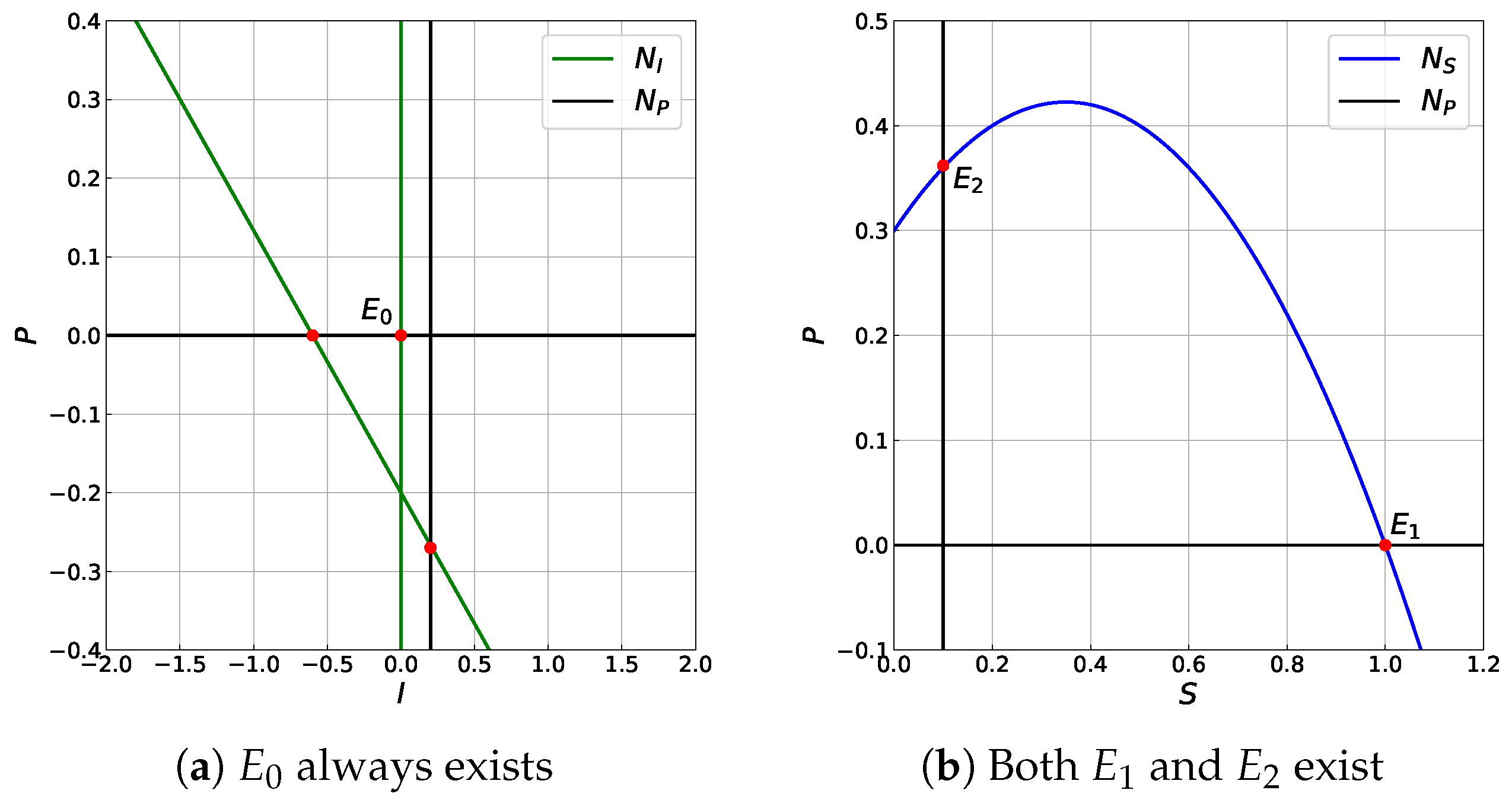
3.3. The Existence of Equilibrium Point

From model (12), we can determine the nullclines of the susceptible prey, infected prey and predator, which are respectively denoted by $N_S,N_I$ and $N_P$ and are defined by the following sets

$$\begin{array}{cc}\hfill N_S:=& \left\{(S,I,P):S=0\vee S+(1+\eta )I+\frac{P}{\kappa +S}=1\right\},\hfill \\ \hfill N_I:=& \left\{(S,I,P):I=0\vee S=\frac{\delta }{\eta }+\frac{mP}{\eta (\omega +I)}\right\},\hfill \\ \hfill N_P:=& \left\{(S,I,P):P=0\vee \frac{\mu S}{\kappa +S}+\frac{\beta I}{\omega +I}=q\right\}.\hfill \end{array}$$

Since we are only interested in solutions that satisfy biological conditions, we only consider equilibrium points that satisfy $N_S\cap N_I\cap N_P\subset {\mathbb{R}}_{+}^3$. We can obviously identify that the infected prey and predator are extinct if the susceptible prey is zero. Therefore, the following lemma shows that the origin is the only equilibrium point when $N_S=\left\{(S,I,P):S=0\right\}$.

Lemma 6.

If $N_S:=\left\{(S,I,P):S=0\right\}$ then the origin $E_0=(0,0,0)$ is the only equilibrium point of model (12).

Proof. 

For $N_S:=\left\{(S,I,P):S=0\right\}$, the equilibrium point is defined by $N_I\cap N_P\cap {\mathbb{R}}_{+}^3$, where

$$\begin{array}{cc}\hfill N_I:=& \left\{(S,I,P):I=0\vee \frac{\delta }{\eta }+\frac{mP}{\eta (\omega +I)}=0\right\},\hfill \\ \hfill N_P:=& \left\{(S,I,P):P=0\vee \frac{\beta I}{\omega +I}=q\right\}.\hfill \end{array}$$

Since $\frac{\delta }{\eta }+\frac{mP}{\eta (\omega +I)}\ne 0$, then $I=0$ is the only nullcline of I. By substituting $I=0$ to $N_P$, we have $N_P=\left\{(S,I,P):P=0\vee q=0\right\}$. $P=0$ is the only nullcline of P because $q\ne 0$. Thus, $E_0=(0,0,0)$ is the only equilibrium point. □

Now, we will investigate the equilibrium point when $S\ne 0$. Notice that if $N_I:=\left\{(S,I,P):I=0\right\}$, then $N_S\cap N_P\cap {\mathbb{R}}_{+}^3$ is the equilibrium point of model (12) where

$$N_S:=\left\{(S,I,P):S+\frac{P}{\kappa +S}=1\right\},\mathrm{and}{N}_P:=\left\{(S,I,P):P=0\vee \frac{\mu S}{\kappa +S}=q\right\}.$$

Immediately we recognize two equilibrium points as follows:

• The extinction of infected prey and predator point: $E_1=(1,0,0)$, which always exists.
• The infected prey free point $E_2=\left(\widehat{S},0,\widehat{P}\right)$ where $\widehat{S}=\frac{q\kappa }{\mu -q}$ and $\widehat{P}=(1-\widehat{S})(\kappa +\widehat{S})$ which exists if $\mu >(1+\kappa )q$. The condition $\mu >(1+\kappa )q$ is equivalent to condition that the conversion rate of susceptible prey predation into the birth rate of predator is larger than the sum of the death rate of predator and its multiplication with half-saturation constant of predation.

Furthermore, if $N_P=\left\{(S,I,P):P=0\right\}$, we obtain equilibrium points that satisfy $N_S\cap N_I\cap {\mathbb{R}}_{+}^3$ where

$$N_S:=\left\{(S,I,P):S+(1+\eta )I=1\right\},\mathrm{and}{N}_I:=\left\{(S,I,P):I=0\vee S=\frac{\delta }{\eta }\right\}.$$

Thus, we have the extinction of infected prey and predator point $E_1=(1,0,0)$ and the predator-free point $E_3=\left(\tilde{S},\frac{1-\tilde{S}}{1+\eta },0\right)$, where $\tilde{S}=\frac{\delta }{\eta }$. The point $E_3$ exists if $\tilde{S}\in (0,1)$ or $\eta >\delta$, i.e., when the prey infection rate is greater than the infected prey death rate.

By considering the following nullclines

$$\begin{array}{c}{N}_S:=\left\{(S,I,P):S+(1+\eta )I+\frac{P}{\kappa +S}=1\right\},\hfill \\ N_I:=\left\{(S,I,P):S=\frac{\delta }{\eta }+\frac{mP}{\eta (\omega +I)}\right\},N_P:=\left\{(S,I,P):\frac{\mu S}{\kappa +S}+\frac{\beta I}{\omega +I}=q\right\},\hfill \end{array}$$

we obtain the co-existence equilibrium point $E^{*}=\left(S^{*},I^{*},P^{*}\right)$ that satisfies $N_S\cap N_I\cap N_P\cap {\mathbb{R}}_{+}^3$, i.e.,

$$S^{*}=\frac{-a_2\pm \sqrt{D}}{2a_1},I^{*}=\frac{(1-S^{*})(\kappa +S^{*})m-\omega (\eta S^{*}-\delta )}{(\kappa +S^{*})(\eta +1)m+(\eta S^{*}-\delta )},P^{*}=\frac{(\eta S^{*}-\delta )(\omega +I^{*})}{m},$$

where

$$\begin{array}{cccc}\hfill a_1=& (\beta +\mu )m-mq,\hfill & \hfill a_3=& \left((\eta +1)\omega +1\right)mq\kappa -(m\kappa +\delta \omega )\beta \hfill \\ \hfill a_2=& \left(\right(\eta +1)\omega +1)mq+(\eta \omega +m\kappa )\beta \hfill & \hfill D=& a_2^2-4a_1{a}_3\hfill \\ \hfill & -\left(\left(\right(\eta +1)\omega +1)\mu +q\kappa +\beta \right)m\hfill & \hfill \end{array}$$

The existence of $E^{*}$ is described by the following lemma.

Lemma 7.

Suppose that

$$\begin{array}{cccccc}\hfill S_1^{*}=& -\frac{a_2-\sqrt{D}}{2a_1},\hfill & \hfill S_2^{*}=& -\frac{a_2+\sqrt{D}}{2a_1},\hfill & \hfill S_3^{*}=& -\frac{a_2}{2a_1},\hfill \\ \hfill S_{1,2}^{*}\in & \left(\frac{\delta }{\eta },1\right),\hfill & \hfill m>& \frac{\omega (\eta S_j^{*}-\delta )}{(1-S_j^{*})(\kappa +S_j^{*})},j=1,2,\hfill & \hfill a_1{a}_2<& 0.\hfill \end{array}$$

(i) 

If $D<0$, then the co-existence point does not exist.

(ii) 

if $D>0$ and

(a) 

$a_1{a}_3>0$ then there are two co-existence points, i.e., $E_1^{*}=(S_1^{*},I_1^{*},P_1^{*})$ and $E_2^{*}=(S_2^{*},I_2^{*},P_2^{*})$.

(b) 

$a_1{a}_3\le 0$ then $E_1^{*}=(S_1^{*},I_1^{*},P_1^{*})$ is the unique co-existence point.

(iii) 

If $D=0$, then there is a unique co-existence point $E_3^{*}=(S_3^{*},I_3^{*},P_3^{*})$.

Proof. 

Notice if $S_j^{*}\in \left(\frac{\delta }{\eta },1\right)$ and $m>\frac{\omega (\eta S_j^{*}-\delta )}{(1-S_j^{*})(\kappa +S_j^{*})}$ then $I_j^{*}>0$ and $P_j^{*}>0$, $j=1,2$.

(i)

It is clear that if $D<0$ then $S_j^{*}\notin \mathbb{R}$, and thus the co-existence point does not exist.

(ii)

if $D>0$ then $S_j^{*}\in \mathbb{R}$. As a result that $a_1{a}_2<0$, we have $S_1^{*}+S_2^{*}>0$. Furthermore, if

(a)

$a_1{a}_3>0$ then $S_1^{*}{S}_2^{*}>0$. Therefore, we have $S_1^{*}>0$ and $S_2^{*}>0$ and $E_{1,2}^{*}\in {\mathbb{R}}_{+}^3$.

(b)

$a_1{a}_3\le 0$ then $S_1^{*}{S}_2^{*}\le 0$ so that $S_1^{*}>0$ and $S_2^{*}\le 0$.

(iii)

If $D=0$ then $S_3^{*}$ is the only solution for $S_j^{*}$. Furthermore, if $a_1{a}_2<0$ then $S_3^{*}>0$.

Thus, we have the lemma. □

To illustrate the existence of equilibrium point by utilizing the nullclines, we take $\eta =0.95$, $\kappa =0.3$, $\delta =0.2$, $m=0.6$, $\omega =0.6$ $\mu =0.4$, $\beta =0.4$ and $q=0.1$. We note that $E_0$ always exists. Besides $E_0$, there also exist $E_1$ and $E_2$ in ${\mathbb{R}}_{+}^3$, see Figure 1a,b. If we decrease $\eta$ so that $\eta =0.5$, then model (12) has a predator-free point $E_3$, see Figure 1c. Next, to show the existence of co-existence point $\left(E^{*}\right)$, we choose parameter values: $\eta =0.8$, $\delta =0.17$, $m=0.7$, $\omega =0.1$, $\mu =0.5$, $\beta =0.3$ and $q=0.4$. It can be seen in Figure 1d that model (12) with $\kappa =0.6$ has two co-existence points. If we increase $\kappa$ such that $\kappa =0.4$, then we have a unique co-existence point, see Figure 1e. However, if we take $\kappa =1$, then model (12) does not have co-existence point (see Figure 1f).

Figure 1. The existence of equilibrium point of model (12) by utilizing the intersection of nullclines.

3.4. Local Stability of Equilibrium Points

In this part, we investigate the local stability properties of each equilibrium point of model (12). The local stability properties are studied by observing the eigenvalues of the Jacobian matrix at each equilibrium points, and the results are described in the following theorems.

Theorem 5.

The equilibrium point $E_0$ is always a saddle point.

Proof. 

The Jacobian matrix of model (12) evaluated at $E_0$ is

$$J\left(E_0\right)=\left[\begin{array}{ccc}1& 0& 0\\ 0& -\delta & 0\\ 0& 0& -q\end{array}\right].$$

The eigenvalues of this Jacobian matrix are ${\lambda }_1=1$, ${\lambda }_2=-\delta$ and ${\lambda }_3=-q$. Thus, $|arg\left({\lambda }_1\right)|=0<\frac{\alpha \pi }{2}$ and $|arg\left({\lambda }_2\right)|=|arg\left({\lambda }_3\right)|=\pi >\frac{\alpha \pi }{2}$. Based on Matignon condition in Theorem 2, we conclude that $E_0$ is a saddle point. □

Theorem 6.

The equilibrium point $E_1$ is:

(i) 

locally asymptotically stable if $\eta <\delta$ and $\mu <(1+\kappa )q$.

(ii) 

a saddle point if $\eta >\delta$ or $\mu >(1+\kappa )q$.

Proof. 

The Jacobian matrix at $E_1$ is

$$J\left(E_1\right)=\left[\begin{array}{ccc}-1& -(\eta +1)& -\frac{1}{\kappa +1}\\ 0& \eta -\delta & 0\\ 0& 0& \frac{\mu }{\kappa +1}-q\end{array}\right].$$

$J\left(E_1\right)$ has eigenvalues: ${\lambda }_1=-1$, ${\lambda }_2=\eta -\delta$ and ${\lambda }_3=\frac{\mu }{\kappa +1}-q$. We have $|arg\left({\lambda }_1\right)|=\pi >\frac{\alpha \pi }{2}$. Hence, the stability of $E_1$ depends on ${\lambda }_{2,3}$.

(i)

If $\eta <\delta$ and $\mu <(1+\kappa )q$, then $|arg\left({\lambda }_2\right)|=\pi >\frac{\alpha \pi }{2}$ and $|arg\left({\lambda }_3\right)|=\pi >\frac{\alpha \pi }{2}$. Due to Matignon condition at Theorem 2, $E_1$ is locally asymptotically stable.

(ii)

If $\eta >\delta$ then $|arg\left({\lambda }_2\right)|=0<\frac{\alpha \pi }{2}$. In addition, if $\mu >(1+\kappa )q$ then $|arg\left({\lambda }_3\right)|=0<\frac{\alpha \pi }{2}$. Thus, Theorem 2 says that $E_1$ is a saddle point.

 □

Theorem 7.

Suppose that:

$$\begin{array}{cccc}\hfill \widehat{\eta }=& \frac{\delta }{\widehat{S}}+\frac{m(1-\widehat{S})(\kappa +\widehat{S})}{\omega \widehat{S}},\hfill & \hfill \widehat{\Delta }=& \frac{4(1-\widehat{S})\mu \kappa \widehat{S}}{{(\kappa +\widehat{S})}^2}-{\left(\frac{\kappa -1+2\widehat{S}}{\kappa +\widehat{S}}\right)}^2{\widehat{S}}^2,\hfill \\ \hfill \widehat{\alpha }=& \frac{2}{\pi }{tan}^{-1}\left(\frac{(\kappa +\widehat{S})\sqrt{\widehat{\Delta }}}{(\kappa -1+2\widehat{S})\widehat{S}}\right).\hfill \end{array}$$

The equilibrium point $E_2$ is:

(i) 

locally asymptotically stable if $\eta <\widehat{\eta }$ and

(a) 

$\kappa >1-2\widehat{S}$, or;

(b) 

$\kappa <1-2\widehat{S}$, $\widehat{\Delta }>0$ and $\alpha <\widehat{\alpha }$.

(ii) 

a saddle point if

(a) 

$\eta >\widehat{\eta }$ and $\kappa >1-2\widehat{S}$, or;

(b) 

$\eta >\widehat{\eta }$, $\kappa <1-2\widehat{S}$, $\widehat{\Delta }>0$, and $\alpha <\widehat{\alpha }$, or;

(c) 

$\eta <\widehat{\eta }$, $\kappa <1-2\widehat{S}$, and $\alpha >\widehat{\alpha }$.

Proof. 

The Jacobian matrix of model (12) evaluated at $E_2$ is

$$J\left(E_2\right)=\left[\begin{array}{ccc}-\widehat{S}+\frac{(1-\widehat{S})\widehat{S}}{\kappa +\widehat{S}}& -(1+\eta )\widehat{S}& -\frac{\widehat{S}}{\kappa +\widehat{S}}\\ 0& \left(\eta -\widehat{\eta }\right)\widehat{S}& 0\\ \frac{(1-\widehat{S})\mu \kappa }{\kappa +\widehat{S}}& \frac{\beta (1-\widehat{S})(\kappa +\widehat{S})}{\omega }& 0\end{array}\right],$$

which has eigenvalues: ${\lambda }_1=\left(\eta -\widehat{\eta }\right)\widehat{S}$ and ${\lambda }_{2,3}=-\frac{\widehat{S}}{2}\left(\frac{\kappa -1+2\widehat{S}}{\kappa +\widehat{S}}\right)\pm \frac{\sqrt{\widehat{\Delta }}}{2}$. Notice that if $\eta <\widehat{\eta }$ then $\left|arg\left({\lambda }_1\right)\right|=\pi >\frac{\alpha \pi }{2}$, else if $\eta >\widehat{\eta }$ then $\left|arg\left({\lambda }_1\right)\right|=0<\frac{\alpha \pi }{2}$. Furthermore, if $\kappa >1-2\widehat{S}$ then $\left|arg\left({\lambda }_{2,3}\right)\right|>\frac{\alpha \pi }{2}$ for both $\widehat{\Delta }\ge 0$ and $\widehat{\Delta }<0$. If $\kappa <1-2\widehat{S}$ and $\widehat{\Delta }>0$, then ${\lambda }_{2,3}$ is a pair of complex eigenvalues. Thus, $\left|arg\left({\lambda }_{2,3}\right)\right|>\frac{\alpha \pi }{2}$ is attained if $\alpha <\widehat{\alpha }$. When $\kappa <1-2\widehat{S}$, and $\alpha >\widehat{\alpha }$, we have $\left|arg\left({\lambda }_{2,3}\right)\right|<\frac{\alpha \pi }{2}$ for both $\widehat{\Delta }\le 0$ and $\widehat{\Delta }>0$. Therefore, by Matignon condition in Theorem 2, the theorem is completely proven. □

Theorem 8.

Suppose that: $\tilde{q}=\frac{\mu \tilde{S}}{\kappa +\tilde{S}}+\frac{(1-\tilde{S})\beta }{\omega (1+\eta )+(1-\tilde{S})}$. The predator-free point $E_3$ is locally asymptotically stable if $q>\tilde{q}$ and it is a saddle point if $q<\tilde{q}$.

Proof. 

We compute the Jacobian matrix of model (12) evaluated at $E_3$ and obtain

$$J\left(E_3\right)=\left[\begin{array}{ccc}-\tilde{S}& -(1+\eta )\tilde{S}& -\frac{\tilde{S}}{\kappa +\tilde{S}}\\ \frac{(1-\tilde{S})\eta }{1+\eta }& 0& -\frac{(1-\tilde{S})m}{\omega (1+\eta )+(1-\tilde{S})}\\ 0& 0& \tilde{q}-q\end{array}\right].$$

The eigenvalues of $J\left(E_3\right)$ are ${\lambda }_1=\tilde{q}-q$ and ${\lambda }_{2,3}=\frac{-\tilde{S}\pm \sqrt{(\tilde{S}-4(1-\tilde{S})\eta )\tilde{S}}}{2}$. If $\eta \le \frac{\tilde{S}}{4(1-\tilde{S})}$, then the eigenvalues ${\lambda }_{2,3}$ are always real and negative. Moreover, if $\eta >\frac{\tilde{S}}{4(1-\tilde{S})}$, then ${\lambda }_{2,3}$ are a pair of complex conjugates where $Re\left({\lambda }_{2,3}\right)<0$. Hence, the eigenvalues ${\lambda }_{2,3}$ always satisfy $\left|arg\left({\lambda }_{2,3}\right)\right|>\frac{\alpha \pi }{2}$. Finally, $|arg\left({\lambda }_1\right)|=\pi >\frac{\alpha \pi }{2}$ is achieved if $q>\tilde{q}$. Therefore, the predator-free point $E_3$ is locally asymptotically stable if $q>\tilde{q}$; otherwise it is a saddle point. □

Theorem 9.

Suppose that:

$$\begin{array}{cc}\hfill d_1=& S^{*}-\left(\frac{S^{*}{P}^{*}}{{(\kappa +S^{*})}^2}+\frac{m{I}^{*}{P}^{*}}{{(\omega +I^{*})}^2}\right),\hfill \\ \hfill d_2=& \left[\frac{m{S}^{*}{I}^{*}{\left(P^{*}\right)}^2}{{(\kappa +S^{*})}^2{(\omega +I^{*})}^2}+\frac{\beta m{I}^{*}{P}^{*}}{{(\omega +I^{*})}^2}+\frac{\mu S^{*}{P}^{*}}{{(\kappa +S^{*})}^2}+(\eta +1)\eta S^{*}{I}^{*}\right]-\hfill \\ \hfill & \left[\frac{m{S}^{*}{I}^{*}{P}^{*}}{{(\omega +I^{*})}^2}+\frac{m\beta {\left(I^{*}\right)}^2{P}^{*}}{{(\omega +I^{*})}^3}+\frac{\mu {\left(S^{*}\right)}^2{P}^{*}}{{(\kappa +S^{*})}^3}\right],\hfill \\ \hfill d_3=& \left[\frac{\eta }{\kappa +S^{*}}+\frac{\omega m}{{(\omega +I^{*})}^2}\right]\frac{\beta S^{*}{I}^{*}{P}^{*}}{\omega +I^{*}}-\left[\frac{\beta \eta I^{*}}{\omega +I^{*}}+\frac{(\eta +1)\mu \kappa m}{\kappa +S^{*}}\right]\frac{S^{*}{I}^{*}{P}^{*}}{(\kappa +S^{*})(\omega +I^{*})}-\hfill \\ \hfill & \left[\frac{\mu \kappa }{\kappa +S^{*}}+\frac{\beta \omega }{\omega +I^{*}}\right]\frac{m{S}^{*}{I}^{*}{\left(P^{*}\right)}^2}{{(\kappa +S^{*})}^2{(\omega +I^{*})}^2},\hfill \\ \hfill {\Delta }^{*}=& 18d_1{d}_2{d}_3+{\left(d_1{d}_2\right)}^2-4d_3{d}_1^3-4d_2^3-27d_3^2.\hfill \end{array}$$

The co-existence point $E^{*}=(S^{*},I^{*},P^{*})$ is locally asymptotically stable if one of the following statements is satisfied.

(i) 

${\Delta }^{*}>0$, $d_1>0$, $d_3>0$, and $d_1{d}_2>c{d}_3$.

(ii) 

${\Delta }^{*}<0$, $d_1\ge 0$, $d_2\ge 0$, $d_3>0$, and $0<\alpha <(2/3)$.

(iii) 

${\Delta }^{*}<0$, $d_1<0$, $d_2<0$, and $(2/3)<\alpha <1$.

(iv) 

${\Delta }^{*}<0$, $d_1>0$, $d_2>0$, $d_1{d}_2=d_3$, and $0<\alpha <1$.

Proof. 

The Jacobian matrix of model (12) evaluated at $E^{*}$ is,

$$J\left(E^{*}\right)=\left[\begin{array}{ccc}\frac{S^{*}{P}^{*}}{{(\kappa +S^{*})}^2}-S^{*}& -(\eta +1)S^{*}& -\frac{S^{*}}{\kappa +S^{*}}\\ \eta I^{*}& \frac{m{I}^{*}{P}^{*}}{{(\omega +I^{*})}^2}& -\frac{m{I}^{*}}{\omega +I^{*}}\\ \left[1-\frac{S^{*}}{\kappa +S^{*}}\right]\frac{\mu P^{*}}{\kappa +S^{*}}& \left[1-\frac{I^{*}}{\omega +I^{*}}\right]\frac{\beta P^{*}}{\omega +I^{*}}& 0\end{array}\right].$$

The characteristic equation of $J\left(E^{*}\right)$ is ${\lambda }^3+d_1{\lambda }^2+d_2\lambda +d_3=0$. Using the Routh–Hurwitz condition for a fractional-order dynamical system (See Proposition 1 in [72]), the locally stability conditions of co-existence point $E^{*}=(S^{*},I^{*},P^{*})$ are proven. □

3.5. Global Stability of Equilibrium Points

The global asymptotic stability of the equilibrium point of model (12) is studied. The results are presented in the following theorems.

Theorem 10.

$E_1=(1,0,0)$ is globally asymptotically stable if $max\left\{\frac{\eta }{\delta },\frac{\beta \kappa +\mu }{\kappa q}\right\}<1$.

Proof. 

Consider a Lyapunov function $W_1(S,I,P)=\left[S-1-lnS\right]+\frac{1+\eta }{\eta }I+\frac{1}{\mu }P$. By using Lemma 4, we get

$$\begin{array}{cc}\hfill {}^C{\mathcal{D}}_t^{\alpha }{W}_1(S,I,P)\le & \left(\frac{S-1}{S}\right){}^C{\mathcal{D}}_t^{\alpha }S+\frac{1+\eta }{\eta }{}^C{\mathcal{D}}_t^{\alpha }I+\frac{1}{\mu }{}^C{\mathcal{D}}_t^{\alpha }P\hfill \\ \hfill =& \left(S-1\right)\left[1-S-(1+\eta )I-\frac{P}{\kappa +S}\right]+\frac{1+\eta }{\eta }\left[\eta S-\delta -\frac{mP}{\omega +I}\right]I\hfill \\ \hfill & +\frac{1}{\mu }\left[\frac{\mu S}{\kappa +S}+\frac{\beta I}{\omega +I}-q\right]P\hfill \\ \hfill =& -{(S-1)}^2-\frac{(\delta -\eta )(1+\eta )I}{\eta }+\frac{P}{\kappa +S}-\frac{(1+\eta )mIP}{(\omega +I)\eta }\hfill \\ \hfill & +\frac{\beta IP}{(\omega +I)\mu }-\frac{qP}{\mu }\hfill \\ \hfill \le & -{\left(S-1\right)}^2-\frac{(\delta -\eta )(1+\eta )I}{\eta }+\frac{P}{\kappa }+\frac{\beta P}{\mu }-\frac{qP}{\mu }\hfill \\ \hfill =& -{\left(S-1\right)}^2-\frac{(\delta -\eta )(1+\eta )I}{\eta }-\left(q-\left(\beta +\frac{\mu }{\kappa }\right)\right)\frac{P}{\mu }\hfill \end{array}$$

Thus, ${}^C{\mathcal{D}}_t^{\alpha }{W}_1(S,I,P)\le 0$ when $max\left\{\frac{\eta }{\delta },\frac{\beta \kappa +\mu }{\kappa q}\right\}<1$. According to Lemma 5, it follows that $E_1$ is globally asymptotically stable. □

Theorem 11.

If $\widehat{S}<min\left\{\frac{\delta }{\eta },\frac{\left(\right(1+\eta )m\mu -\beta \eta )\kappa }{\beta \eta }\right\}$ and $\widehat{P}<{\kappa }^2$ then the infected prey extinction point $E_2$ is globally asymptotically stable.

Proof. 

We define a Lyapunov function

$$W_2(S,I,P)=\left[S-\widehat{S}-\widehat{S}ln\frac{S}{\widehat{S}}\right]+\frac{1+\eta }{\eta }I+\frac{\kappa +\widehat{S}}{\mu \kappa }\left[P-\widehat{P}-\widehat{P}ln\frac{P}{\widehat{P}}\right].$$

Based on Lemma 4, we have

$$\begin{array}{cc}\hfill {}^C{\mathcal{D}}_t^{\alpha }{W}_2(S,I,P)\le & \left(\frac{S-\widehat{S}}{S}\right){}^C{\mathcal{D}}_t^{\alpha }S+\frac{1+\eta }{\eta }{}^C{\mathcal{D}}_t^{\alpha }I+\frac{\kappa +\widehat{S}}{\mu \kappa }\left(\frac{P-\widehat{P}}{P}\right){}^C{\mathcal{D}}_t^{\alpha }P\hfill \\ \hfill =& (S-\widehat{S})\left[1-S-(1+\eta )I-\frac{P}{\kappa +S}\right]+\frac{1+\eta }{\eta }\left[\eta S-\delta -\frac{mP}{\omega +I}\right]I\hfill \\ \hfill & +\frac{\kappa +\widehat{S}}{\mu \kappa }(P-\widehat{P})\left[\frac{\mu S}{\kappa +S}+\frac{\beta I}{\omega +I}-q\right]\hfill \\ \hfill =& (S-\widehat{S})\left[-(S-\widehat{S})-(1+\eta )I-\frac{(\kappa +\widehat{S})(P-\widehat{P})-\widehat{P}(S-\widehat{S})}{(\kappa +S)(\kappa +\widehat{S})}\right]\hfill \\ \hfill & +\frac{1+\eta }{\eta }\left[\eta S-\delta -\frac{mP}{\omega +I}\right]I\hfill \\ \hfill & +\frac{\kappa +\widehat{S}}{\mu \kappa }(P-\widehat{P})\left[\frac{\mu \kappa (S-\widehat{S})}{(\kappa +S)(\kappa +\widehat{S})}+\frac{\beta I}{\omega +I}\right]\hfill \\ \hfill =& -{(S-\widehat{S})}^2+\frac{\widehat{P}{(S-\widehat{S})}^2}{(\kappa +S)(\kappa +\widehat{S})}-\left(\frac{\delta }{\eta }-\widehat{S}\right)(1+\eta )I\hfill \\ \hfill & -\left(\frac{(1+\eta )m}{\eta }-\frac{(\kappa +\widehat{S})\beta }{\mu \kappa }\right)\frac{IP}{\omega +I}\hfill \\ \hfill \le & -\left(1-\frac{\widehat{P}}{{\kappa }^2}\right){(S-\widehat{S})}^2-\left(\frac{\delta }{\eta }-\widehat{S}\right)(1+\eta )I\hfill \\ \hfill & -\left(\frac{(1+\eta )m}{\eta }-\frac{(\kappa +\widehat{S})\beta }{\mu \kappa }\right)\frac{IP}{\omega +I}\hfill \end{array}$$

It is clear that ${}^C{\mathcal{D}}_t^{\alpha }{W}_2\left(E_2\right)\le 0$ if $\widehat{S}<min\left\{\frac{\delta }{\eta },\frac{\left(\right(1+\eta )m\mu -\beta \eta )\kappa }{\beta \eta }\right\}$ and $\widehat{P}<{\kappa }^2$. Consequently, Lemma 5 says that $E_2$ is globally asymptotically stable. □

Theorem 12.

If $q>\beta +\frac{\mu \tilde{S}}{\kappa }+\frac{(1+\eta )\mu m\tilde{I}}{\eta \omega }$ then the predator-free point $E_3$ is globally asymptotically stable.

Proof. 

We first write $\tilde{I}=\frac{1-\tilde{S}}{1+\eta }$ and define a Lyapunov function

$$W_3(S,I,P)=\left[S-\tilde{S}-\tilde{S}ln\frac{S}{\tilde{S}}\right]+\frac{1+\eta }{\eta }\left[I-\tilde{I}-\tilde{I}ln\frac{I}{\tilde{I}}\right]+\frac{1}{\mu }P.$$

By using Lemma 4, we obtain

$$\begin{array}{cc}\hfill {}^C{\mathcal{D}}_t^{\alpha }{W}_3(S,I,P)\le & \left(\frac{S-\tilde{S}}{S}\right){}^C{\mathcal{D}}_t^{\alpha }S+\frac{1+\eta }{\eta }\left(\frac{I-\tilde{I}}{I}\right){}^C{\mathcal{D}}_t^{\alpha }I+\frac{1}{\mu }{}^C{\mathcal{D}}_t^{\alpha }P\hfill \\ \hfill =& (S-\tilde{S})\left[1-S-(1+\eta )I-\frac{P}{\kappa +S}\right]+\frac{1+\eta }{\eta }\left(I-\tilde{I}\right)\left[\eta S-\delta -\frac{mP}{\omega +I}\right]\hfill \\ \hfill & +\frac{1}{\mu }\left[\frac{\mu S}{\kappa +S}+\frac{\beta I}{\omega +I}-q\right]P\hfill \\ \hfill =& (S-\tilde{S})\left[\tilde{S}+(1+\eta )\tilde{I}-S-(1+\eta )I-\frac{P}{\kappa +S}\right]\hfill \\ \hfill & +\frac{1+\eta }{\eta }\left(I-\tilde{I}\right)\left[\eta S-\eta \tilde{S}-\frac{mP}{\omega +I}\right]+\frac{1}{\mu }\left[\frac{\mu S}{\kappa +S}+\frac{\beta I}{\omega +I}-q\right]P\hfill \\ \hfill =& -{(S-\tilde{S})}^2+\frac{\tilde{S}P}{\kappa +S}-\left(\frac{(1+\eta )m}{\eta }-\frac{\beta }{\mu }\right)\frac{IP}{\omega +I}+\frac{(1+\eta )m\tilde{I}P}{(\omega +I)\eta }-\frac{qP}{\mu }\hfill \\ \hfill \le & -{(S-\tilde{S})}^2+\frac{\tilde{S}P}{\kappa }+\frac{\beta P}{\mu }+\frac{(1+\eta )m\tilde{I}P}{\eta \omega }-\frac{qP}{\mu }\hfill \\ \hfill =& -{(S-\tilde{S})}^2-\left(\frac{q}{\mu }-\frac{\beta }{\mu }-\frac{\tilde{S}}{\kappa }-\frac{(1+\eta )m\tilde{I}}{\eta \omega }\right)P\hfill \end{array}$$

If $q>\beta +\frac{\mu \tilde{S}}{\kappa }+\frac{(1+\eta )\mu m\tilde{I}}{\eta \omega }$, then we have ${}^C{\mathcal{D}}_t^{\alpha }{W}_3(S,I,P)\le 0$. It follows from Lemma 5 that $E_3$ is globally asymptotically stable. □

Theorem 13.

Suppose that

$$\begin{array}{cc}\hfill {\phi }_1=& \frac{q{P}^{*}}{\mu }+\frac{(1+\eta )\delta I^{*}}{\eta },\hfill \\ \hfill {\phi }_2=& min\left\{I^{*}+\eta I^{*}-1,\frac{\delta }{\eta },\frac{q\eta \omega -(1+\eta )m\kappa I^{*}}{\eta \omega }\right\}.\hfill \end{array}$$

The co-existence point $E^{*}$ is globally asymptotically stable if $\mu >\frac{\beta }{m}$ and ${\phi }_1<S^{*}<{\phi }_2$.

Proof. 

Consider a positive Lyapunov function

$$W_4\left(E^{*}\right)=\left[S-S^{*}-S^{*}ln\frac{S}{S^{*}}\right]+\frac{1+\eta }{\eta }\left[I-I^{*}-I^{*}ln\frac{S}{I^{*}}\right]+\frac{1}{\mu }\left[P-P^{*}-P^{*}ln\frac{P}{P^{*}}\right].$$

By utilizing Lemma 4, one has

$$\begin{array}{cc}\hfill {}^C{\mathcal{D}}_t^{\alpha }{W}_4\left(E^{*}\right)\le & \left(\frac{S-S^{*}}{S}\right){}^C{\mathcal{D}}_t^{\alpha }S+\frac{1+\eta }{\eta }\left(\frac{I-I^{*}}{I}\right){}^C{\mathcal{D}}_t^{\alpha }I+\frac{1}{\mu }\left(\frac{P-P^{*}}{P}\right){}^C{\mathcal{D}}_t^{\alpha }P\hfill \\ \hfill =& (S-S^{*})\left[1-S-(1+\eta )I-\frac{P}{\kappa +S}\right]\hfill \\ \hfill & +\frac{1+\eta }{\eta }\left(I-I^{*}\right)\left[\eta S-\delta -\frac{mP}{\omega +I}\right]+\frac{1}{\mu }(P-P^{*})\left[\frac{\mu S}{\kappa +S}+\frac{\beta I}{\omega +I}-q\right]\hfill \\ \hfill =& -S^2-((1+\eta )I^{*}-(1+S^{*}))S-\left(\frac{\delta }{\eta }-S^{*}\right)(1+\eta )I+\frac{S^{*}P}{\kappa +S}\hfill \\ \hfill & +\frac{(1+\eta )\delta I^{*}}{\eta }-\left(\frac{(1+\eta )m}{\eta }-\frac{\beta }{\mu }\right)\frac{IP}{\omega +I}+\frac{(1+\eta )m{I}^{*}P}{\eta (\omega +I)}-\frac{qP}{\mu }\hfill \\ \hfill & -\frac{P^{*}S}{\kappa +S}-\frac{\beta P^{*}I}{\mu (\omega +I)}-S^{*}+\frac{q{P}^{*}}{\mu }\hfill \\ \hfill \le & -((1+\eta )I^{*}-(1+S^{*}))S-\left(\frac{\delta }{\eta }-S^{*}\right)(1+\eta )I-\left(m-\frac{\beta }{\mu }\right)\frac{IP}{\omega +I}\hfill \\ \hfill & -\left(\frac{q}{\mu }-\frac{S^{*}}{\kappa }-\frac{(1+\eta )m{I}^{*}}{\eta \omega }\right)P-\left(S^{*}-\frac{q{P}^{*}}{\mu }-\frac{(1+\eta )\delta I^{*}}{\eta }\right).\hfill \end{array}$$

Obviously, ${}^C{\mathcal{D}}_t^{\alpha }{W}_4\left(E^{*}\right)\le 0$ whenever $\mu >\frac{\beta }{m}$ and ${\phi }_1<S^{*}<{\phi }_2$. Thus, by applying Lemma 5, we can conclude that $E^{*}$ is globally asymptotically stable. □

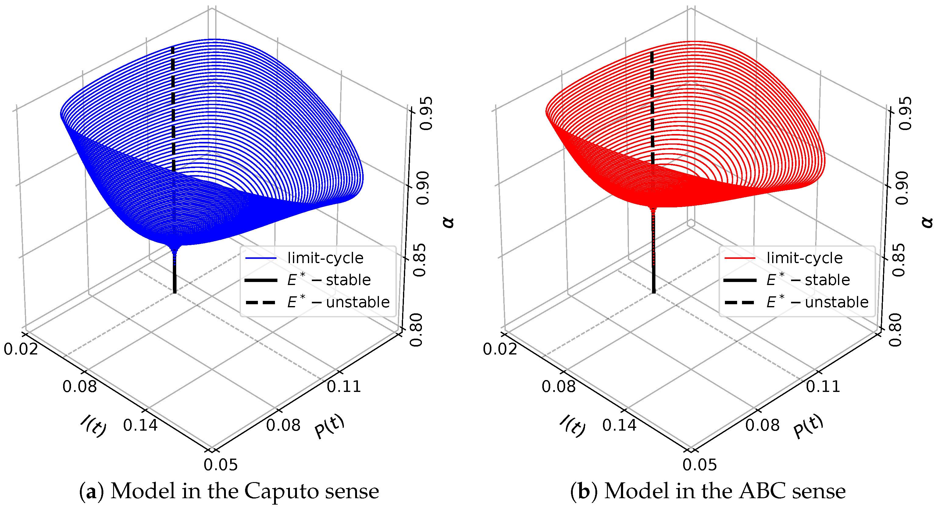
3.6. The Existence of Hopf Bifurcation

One of the interesting phenomena in studying the predator–prey model is the occurrence of Hopf bifurcation. This circumstance arises when the stability of an equilibrium point changes and a limit-cycle appears simultaneously as a parameter is varied [73,74]. In a system of first order differential equations, the occurrence of Hopf bifurcation is indicated by the appearance of purely imaginary eigenvalues of the Jacobian matrix. If we vary the bifurcation parameter, then the sign of the real part of the complex eigenvalues changes [75]; and therefore the stability properties of the equilibrium point also changes. In a fractional-order system, this bifurcation also occurs when the order of fractional derivative $\left(\alpha \right)$ is varied [76]. It is shown in [77,78] that a 3rd-dimensional fractional-order system undergoes a Hopf bifurcation around an equilibrium point if eigenvalues ${\lambda }_{1,2,3}$ of its Jacobian matrix evaluated at the equilibrium point satisfy the following conditions:

• ${\lambda }_1<0$ and ${\lambda }_{2,3}=\theta \pm \omega i$ where $\theta >0$;
• $m\left({\alpha }^{*}\right)={\alpha }^{*}\pi /2-{min}_{1\le i\le 3}\left|arg\left({\lambda }_i\right)\right|=0$;
• ${\left.\frac{dm\left(\alpha \right)}{d\alpha }\right|}_{\alpha ={\alpha }^{*}}\ne 0$.

When $\alpha$ crosses ${\alpha }^{*}=(2/\pi ){tan}^{-1}(\omega /\theta )$, the equilibrium point changes its stability and is accompanied by the appearance of a stable limit-cycle. Since the fractional-order system has no periodic orbits [79], the limit-cycle is not a periodic solution, but it is a nearby solution that converges to periodic signals [76,80].

4. Eco-Epidemic Model in the Atangana–Baleanu Sense

If the fractional-order eco-epidemic model (5) is expressed in the Atangana–Baleanu derivative in Caputo (ABC) sense, then we obtain

$$\begin{array}{cc}\hfill {}^{ABC}{\mathcal{D}}_t^{\alpha }S=& \left[1-S-(1+\eta )I-\frac{P}{\kappa +S}\right]S,\hfill \\ \hfill {}^{ABC}{\mathcal{D}}_t^{\alpha }I=& \left[\eta S-\delta -\frac{mP}{\omega +I}\right]I,\hfill \\ \hfill {}^{ABC}{\mathcal{D}}_t^{\alpha }P=& \left[\frac{\mu S}{\kappa +S}+\frac{\beta I}{\omega +I}-q\right]P.\hfill \end{array}$$

(16)

By Theorem 1, the solution of model (16) can be expressed in the following Volterra-type integral equation

$$\begin{array}{cc}\hfill S\left(t\right)-S\left(0\right)=& \frac{1-\alpha }{B\left(\alpha \right)}{G}_1(t,S)+\frac{\alpha }{B\left(\alpha \right)\Gamma \left(\alpha \right)}{\int }_0^t{(t-s)}^{\alpha -1}{G}_1(s,S)ds,\hfill \\ \hfill I\left(t\right)-I\left(0\right)=& \frac{1-\alpha }{B\left(\alpha \right)}{G}_2(t,I)+\frac{\alpha }{B\left(\alpha \right)\Gamma \left(\alpha \right)}{\int }_0^t{(t-s)}^{\alpha -1}{G}_2(s,I)ds,\hfill \\ \hfill P\left(t\right)-P\left(0\right)=& \frac{1-\alpha }{B\left(\alpha \right)}{G}_3(t,P)+\frac{\alpha }{B\left(\alpha \right)\Gamma \left(\alpha \right)}{\int }_0^t{(t-s)}^{\alpha -1}{G}_3(s,P)ds,\hfill \end{array}$$

(17)

where

$$\begin{array}{cc}\hfill G_1(t,S)=& \left[1-S\left(t\right)-(1+\eta )I\left(t\right)-\frac{P\left(t\right)}{\kappa +S\left(t\right)}\right]S\left(t\right),\hfill \\ \hfill G_2(t,S)=& \left[\eta S\left(t\right)-\delta -\frac{mP\left(t\right)}{\omega +I\left(t\right)}\right]I\left(t\right),\hfill \\ \hfill G_3(t,S)=& \left[\frac{\mu S\left(t\right)}{\kappa +S\left(t\right)}+\frac{\beta I\left(t\right)}{\omega +I\left(t\right)}-q\right]P\left(t\right).\hfill \end{array}$$

The existence and uniqueness of the solutions of model (16) will be investigated in the following sub-section.

Existence and Uniqueness

To prove the existence and uniqueness of solutions of model (16), we first show that the kernels $G_i(t,S),i=1,2,3$ satisfy the Lipschitz condition. Suppose that $S,\overline{S},I,\overline{I},P$ and $\overline{P}$ are functions that satisfy $∥S∥\le a_1$, $∥\overline{S}∥\le a_2$, $∥I∥\le b_1$, $∥\overline{I}∥\le b_2$, $∥P∥\le c_1$ and $∥\overline{P}∥\le c_2$. For the kernel $G_1(t,S)=\left(1-S-(1+\eta )I-\frac{P}{\kappa +S}\right)S$ and two functions S and $\overline{S}$, we get

$$\begin{array}{c}∥G_1(t,S)-G_1(t,\overline{S})∥\hfill \\ \hfill \begin{array}{cc}\hfill =& ∥S-S^2-(1+\eta )SI-\frac{SP}{\kappa +S}-\left(\overline{S}-{\overline{S}}^2-(1+\eta )\overline{S}I-\frac{\overline{S}P}{\kappa +S}\right)∥\hfill \\ \hfill =& ∥S-S^2-(1+\eta )SI-\frac{SP}{\kappa +S}-\overline{S}+{\overline{S}}^2+(1+\eta )\overline{S}I+\frac{\overline{S}P}{\kappa +\overline{S}}∥\hfill \\ \hfill =& ∥\left(S-\overline{S}\right)-\left(S^2-{\overline{S}}^2\right)-\left((1+\eta )SI-(1+\eta )\overline{S}I\right)-\left(\frac{SP}{\kappa +S}-\frac{\overline{S}P}{\kappa +\overline{S}}\right)∥\hfill \\ \hfill =& ∥\left(S-\overline{S}\right)-\left(S+\overline{S}\right)\left(S-\overline{S}\right)-(1+\eta )I\left(S-\overline{S}\right)-\left(\frac{SP(\kappa +\overline{S})-\overline{S}P(\kappa +S)}{(\kappa +S)(\kappa +\overline{S})}\right)∥\hfill \\ \hfill \le & ∥S-\overline{S}∥+(a_1+a_2)∥S-\overline{S}∥+(1+\eta )b_1∥S-\overline{S}∥+\frac{c_1}{\kappa }∥S-\overline{S}∥\hfill \\ \hfill =& \left(1+a_1+a_2+(1+\eta )b_1+\frac{c_1}{\kappa }\right)∥S-\overline{S}∥\hfill \\ \hfill =& g_1∥S-\overline{S}∥,\hfill \end{array}\end{array}$$

(18)

where $g_1=1+a_1+a_2+(1+\eta )b_1+\frac{c_1}{\kappa }$. Hence, the Lipschitz condition holds for $G_1(t,S)$. In a similar manner, we can show that

$$\begin{array}{cc}\hfill ∥G_2(t,I)-G_2(t,\overline{I})∥\le & g_2∥I-\overline{I}∥,\hfill \\ \hfill ∥G_3(t,P)-G_3(t,\overline{P})∥\le & g_3∥P-\overline{P}∥,\hfill \end{array}$$

(19)

where $g_2=a_1\eta +\delta +\frac{c_{1}m}{\omega }$ and $g_3=\frac{a_1\mu }{\kappa }+\frac{b_1\beta }{\omega }+q$. Hence, the Lipschitz condition also holds for kernels $G_2(t,I)$ and $G_3(t,P)$. Furthermore, $G_2(t,I)$ and $G_3(t,P)$ are contracted if $0\le g_2<1$ and $0\le g_3<1$, respectively.

Now, we investigate the existence of solutions of model (16) by employing the fixed-point theorem. For this purpose, we start by writing Equation (17) in the following recursive formulae

$$\begin{array}{cc}\hfill S_n\left(t\right)=& \frac{1-\alpha }{B\left(\alpha \right)}{G}_1(t,S_{n-1})+\frac{\alpha }{B\left(\alpha \right)\Gamma \left(\alpha \right)}{\int }_0^t{(t-s)}^{\alpha -1}{G}_1(s,S_{n-1})ds,\hfill \\ \hfill I_n\left(t\right)=& \frac{1-\alpha }{B\left(\alpha \right)}{G}_2(t,I_{n-1})+\frac{\alpha }{B\left(\alpha \right)\Gamma \left(\alpha \right)}{\int }_0^t{(t-s)}^{\alpha -1}{G}_2(s,I_{n-1})ds,\hfill \\ \hfill P_n\left(t\right)=& \frac{1-\alpha }{B\left(\alpha \right)}{G}_3(t,P_{n-1})+\frac{\alpha }{B\left(\alpha \right)\Gamma \left(\alpha \right)}{\int }_0^t{(t-s)}^{\alpha -1}{G}_3(s,P_{n-1})ds.\hfill \end{array}$$

(20)

The associated initial conditions along with Equation (20) are $S_0\left(t\right)=S\left(0\right),I_0\left(t\right)=I\left(0\right)$, and $P_0\left(t\right)=P\left(0\right)$. Next, from Equation (20), we have the difference expression of successive terms as follows.

$$\begin{array}{cc}\hfill {\Phi }_{1,n}\left(t\right)=& S_n\left(t\right)-S_{n-1}\left(t\right)\hfill \\ \hfill =& \frac{1-\alpha }{B\left(\alpha \right)}\left(G_1(t,S_{n-1})-G_1(t,S_{n-2})\right)\hfill \\ \hfill & +\frac{\alpha }{B\left(\alpha \right)\Gamma \left(\alpha \right)}{\int }_0^t{(t-s)}^{\alpha -1}\left(G_1(s,S_{n-1})-G_1(s,S_{n-2})\right)ds,\hfill \\ \hfill {\Phi }_{2,n}\left(t\right)=& I_n\left(t\right)-I_{n-1}\left(t\right)\hfill \\ \hfill =& \frac{1-\alpha }{B\left(\alpha \right)}\left(G_2(t,I_{n-1})-G_2(t,I_{n-2})\right)\hfill \\ \hfill & +\frac{\alpha }{B\left(\alpha \right)\Gamma \left(\alpha \right)}{\int }_0^t{(t-s)}^{\alpha -1}\left(G_2(s,I_{n-1})-G_2(s,I_{n-2})\right)ds,\hfill \\ \hfill {\Phi }_{3,n}\left(t\right)=& P_n\left(t\right)-P_{n-1}\left(t\right)\hfill \\ \hfill =& \frac{1-\alpha }{B\left(\alpha \right)}\left(G_3(t,P_{n-1})-G_3(t,P_{n-2})\right)\hfill \\ \hfill & +\frac{\alpha }{B\left(\alpha \right)\Gamma \left(\alpha \right)}{\int }_0^t{(t-s)}^{\alpha -1}\left(G_3(s,P_{n-1})-G_3(s,P_{n-2})\right)ds.\hfill \end{array}$$

(21)

Based on Equation (21), we have that

$$S_n\left(t\right)=\sum _{i=1}^n{\Phi }_{1,i}\left(t\right),I_n\left(t\right)=\sum _{i=1}^n{\Phi }_{2,i}\left(t\right),\mathrm{and}{P}_n\left(t\right)=\sum _{i=1}^n{\Phi }_{3,i}\left(t\right).$$

(22)

By using (18) and (19), we can show that the norm of both sides in (21) fulfill the following relations

$$\begin{array}{cc}\hfill ∥{\Phi }_{1,n}\left(t\right)∥\le & \frac{1-\alpha }{B\left(\alpha \right)}{g}_1∥{\Phi }_{1,n-1}∥+\frac{\alpha }{B\left(\alpha \right)\Gamma \left(\alpha \right)}{g}_1{\int }_0^t∥{\Phi }_{1,n-1}\left(s\right)∥{(t-s)}^{\alpha -1}ds,\hfill \\ \hfill ∥{\Phi }_{2,n}\left(t\right)∥\le & \frac{1-\alpha }{B\left(\alpha \right)}{g}_2∥{\Phi }_{2,n-1}∥+\frac{\alpha }{B\left(\alpha \right)\Gamma \left(\alpha \right)}{g}_2{\int }_0^t∥{\Phi }_{2,n-1}\left(s\right)∥{(t-s)}^{\alpha -1}ds,\hfill \\ \hfill ∥{\Phi }_{3,n}\left(t\right)∥\le & \frac{1-\alpha }{B\left(\alpha \right)}{g}_3∥{\Phi }_{3,n-1}∥+\frac{\alpha }{B\left(\alpha \right)\Gamma \left(\alpha \right)}{g}_3{\int }_0^t∥{\Phi }_{3,n-1}\left(s\right)∥{(t-s)}^{\alpha -1}ds.\hfill \end{array}$$

(23)

Now, by applying (23), the existence and uniqueness of model (16) are shown by the following theorem.

Theorem 14.

Model (16) has a unique solution if we can find $t_{max}$ such that

$$\frac{(1-\alpha )g_i}{B\left(\alpha \right)}+\frac{t_{max}^{\alpha }{g}_i}{B\left(\alpha \right)\Gamma \left(\alpha \right)}<1,i=1,2,3$$

(24)

Proof. 

We assume that $S\left(t\right)$, $I\left(t\right)$ and $P\left(t\right)$ are bounded functions, and hence the Lipschitz condition is satisfied. From Equation (23) we can get the following inequalities.

$$\begin{array}{cc}\hfill ∥{\Phi }_{1,n}\left(t\right)∥\le & ∥S_0∥{\left(\frac{(1-\alpha )g_1}{B\left(\alpha \right)}+\frac{t^{\alpha }{g}_1}{B\left(\alpha \right)\Gamma \left(\alpha \right)}\right)}^n,\hfill \\ \hfill ∥{\Phi }_{2,n}\left(t\right)∥\le & ∥I_0∥{\left(\frac{(1-\alpha )g_2}{B\left(\alpha \right)}+\frac{t^{\alpha }{g}_2}{B\left(\alpha \right)\Gamma \left(\alpha \right)}\right)}^n,\hfill \\ \hfill ∥{\Phi }_{3,n}\left(t\right)∥\le & ∥P_0∥{\left(\frac{(1-\alpha )g_3}{B\left(\alpha \right)}+\frac{t^{\alpha }{g}_3}{B\left(\alpha \right)\Gamma \left(\alpha \right)}\right)}^n.\hfill \end{array}$$

(25)

Therefore, the existence and smoothness of the solution presented in Equation (22) are proven since $∥{\Phi }_{1,n}\left(t\right)∥\to 0$, $∥{\Phi }_{2,n}\left(t\right)∥\to 0$ and $∥{\Phi }_{3,n}\left(t\right)∥\to 0$ as $n\to \infty$ and $t=t_{max}$. To show that the functions which satisfy Equation (17) are the solutions of Equation (16), we suppose that

$$\begin{array}{cc}\hfill S\left(t\right)-S\left(0\right)=& S_n\left(t\right)-{{\rm Y}}_{1,n}\left(t\right),\hfill \\ \hfill I\left(t\right)-I\left(0\right)=& I_n\left(t\right)-{{\rm Y}}_{2,n}\left(t\right),\hfill \\ \hfill P\left(t\right)-P\left(0\right)=& P_n\left(t\right)-{{\rm Y}}_{3,n}\left(t\right),\hfill \end{array}$$

(26)

where ${{\rm Y}}_{i,n}\left(t\right),i=1,2,3$ are the remainder terms of series solutions. The norm of ${{\rm Y}}_{1,n}\left(t\right)$ satisfies

$$\begin{array}{cc}\hfill ∥{{\rm Y}}_{1,n}\left(t\right)∥\le & \frac{1-\alpha }{B\left(\alpha \right)}∥G_1(t,S)-G_1(t,S_{n-1})∥\hfill \\ \hfill & +\frac{\alpha }{B\left(\alpha \right)\Gamma \left(\alpha \right)}{\int }_0^t∥G_1(s,S)-G_1(s,S_{n-1})∥{(t-s)}^{\alpha -1}ds,\hfill \\ \hfill \le & ∥S-S_{n-1}∥\left(\frac{1-\alpha }{B\left(\alpha \right)}+\frac{t^{\alpha }}{B\left(\alpha \right)\Gamma \left(\alpha \right)}\right)g_1.\hfill \end{array}$$

(27)

By applying this relation iteratively, we get at $t=t_{max}$

$$∥{{\rm Y}}_{1,n}\left(t\right)∥\le a_1{\left(\frac{1-\alpha }{B\left(\alpha \right)}+\frac{t_{max}^{\alpha }}{B\left(\alpha \right)\Gamma \left(\alpha \right)}\right)}^{n+1}{g}_1^{n+1}.$$

(28)

For $n\to \infty$, we obtain $∥{{\rm Y}}_{1,n}\left(t\right)∥\to 0$. Applying the similar manner, we have $∥{{\rm Y}}_{2,n}\left(t\right)∥\to 0$ and $∥{{\rm Y}}_{3,n}\left(t\right)∥\to 0$. Hence, the functions which satisfy Equation (17) are the solutions of Equation (16).

Now, we show the uniqueness of solutions of Equation (16). For this aim, we suppose that $S^{*}\left(t\right),I^{*}\left(t\right)$ and $P^{*}\left(t\right)$ are another solution of Equation (16). Then, we have

$$\begin{array}{cc}\hfill S\left(t\right)-S^{*}\left(t\right)=& \frac{1-\alpha }{B\left(\alpha \right)}(G_1(t,S)-G_1(t,S^{*}))\hfill \\ \hfill & +\frac{\alpha }{B\left(\alpha \right)\Gamma \left(\alpha \right)}{\int }_0^t(G_1(s,S)-G_1(s,S^{*})){(t-s)}^{\alpha -1}ds.\hfill \end{array}$$

(29)

Taking the norm for both sides and using the same procedures as in (23) and (25), we obtain

$$∥S\left(t\right)-S^{*}\left(t\right)∥\left(1-\frac{(1-\alpha )g_1}{B\left(\alpha \right)}-\frac{t^{\alpha }{g}_1}{B\left(\alpha \right)\Gamma \left(\alpha \right)}\right)\le 0.$$

(30)

For $t=t_{max}$, we have (24). Hence, $∥S\left(t\right)-S^{*}\left(t\right)∥=0$ and consequently $S\left(t\right)=S^{*}\left(t\right)$. In the same way, we can show that $I\left(t\right)=I^{*}\left(t\right)$ and $P\left(t\right)=P^{*}\left(t\right)$. Hence, the uniqueness of the solution of Equation (16) is proven. □

5. Numerical Simulations

In this section, we present some results of our numerical simulations for the fractional-order eco-epidemic models in both Caputo sense (12) and ABC sense (16). For this aim, we solve the model in Caputo sense (12) using the predictor–corrector scheme developed by Diethelm et al. [81], while the model in ABC sense (16) is solved by applying the predictor–corrector scheme proposed by Baleanu et al. [82]. Since the field data are not available, the simulations are performed by using some hypothetical parameter values.

We first perform simulation by setting the parameter values as follows:

$$\eta =0.25,\kappa =0.5,\delta =0.3,m=0.6,\omega =0.6,\mu =0.4,\beta =0.4,q=0.3,\alpha =0.9.$$

(31)

Using these parameter values, the eco-epidemic model with fractional-order derivative in both Caputo sense (12) and ABC sense (16) have two equilibrium points, i.e., $E_0$ and $E_1$. Based on the analysis for the model in Caputo sense (12), it is shown that $E_0$ is a saddle point and $E_1$ is asymptotically stable. This behavior is confirmed by our numerical simulation shown in Figure 2. If we modify the parameter values in (31) such that $\eta =0.35$ and $q=0.2$, then, in addition to $E_0$ and $E_1$, the model also has equilibrium points $E_2$ and $E_3$. All of these equilibrium points are unstable except $E_2$. The stability of $E_2$ is clearly observed in Figure 3. Now, some parameter values in (31) are replaced by $\eta =0.95$, $\delta =0.2$ and $q=0.4$. Under these parameter values, the model has three equilibrium points, i.e., $E_0$, $E_1$ and $E_3$. The previous analysis for the model in Caputo sense shows that $E_0$ and $E_1$ are unstable, while $E_3$ is asymptotically stable. Such stability behavior can be seen in Figure 4. Furthermore, in Figure 2, Figure 3 and Figure 4, the numerical solutions of model in the Caputo sense are compared to those of models in ABC sense. It is observed that the phase portraits and time series of both models have similar dynamical behavior. To see the difference between the solutions of the two models, we perform some simulations using the same parameter values as in Figure 2, Figure 3 and Figure 4, but with varying value of $\alpha$. The time series of solutions obtained from those simulations are plotted in Figure 5, Figure 6 and Figure 7. In these simulations, although the value of $\alpha$ does not affect the stability of the equilibrium point, Figure 5, Figure 6 and Figure 7 show that the value of $\alpha$ greatly affects the rate of convergence in reaching the equilibrium point. Indeed, when $\alpha =1$, the eco-epidemic model with fractional derivative in the Caputo sense and model with fractional derivative in the ABC sense have solutions that coincide with each other.

Figure 2. Numerical simulation of the eco-epidemic model with parameter values: $\eta =0.25$, $\kappa =0.5$, $\delta =0.3$, $m=0.6$, $\omega =0.6$, $\mu =0.4$, $\beta =0.4$, $q=0.3$ and $\alpha =0.9$.

Figure 3. Numerical simulation of the eco-epidemic model with parameter values: $\eta =0.35$, $\kappa =0.5$, $\delta =0.3$, $m=0.6$, $\omega =0.6$, $\mu =0.4$, $\beta =0.4$, $q=0.2$ and $\alpha =0.9$.

Figure 4. Numerical simulation of the eco-epidemic model with parameter values: $\eta =0.95$, $\kappa =0.5$, $\delta =0.2$, $m=0.6$, $\omega =0.6$, $\mu =0.4$, $\beta =0.4$, $q=0.4$ and $\alpha =0.9$.

Figure 5. Time series of solutions of the eco-epidemic model (5) with fractional derivative in the Caputo sense and fractional derivative in ABC sense. The parameter values are $\eta =0.35$, $\kappa =0.5$, $\delta =0.3$, $m=0.6$, $\omega =0.6$, $\mu =0.4$, $\beta =0.4$ and $q=0.2$.

Figure 6. Time series of solutions of the eco-epidemic model (5) with fractional derivative in the Caputo sense and fractional derivative in ABC sense. The parameter values are $\eta =0.35$, $\kappa =0.5$, $\delta =0.3$, $m=0.6$, $\omega =0.6$, $\mu =0.4$, $\beta =0.4$ and $q=0.2$.

Figure 7. Time series of solutions of the eco-epidemic model (5) with fractional derivative in the Caputo sense and fractional derivative in ABC sense. The parameter values are $\eta =0.95$, $\kappa =0.5$, $\delta =0.2$, $m=0.6$, $\omega =0.6$, $\mu =0.4$, $\beta =0.4$ and $q=0.4$.

Next, we perform simulation using the following parameter values:

$$\eta =0.8,\kappa =0.01,\delta =0.17,m=0.7,\omega =0.1,\mu =0.2,\beta =0.27,q=0.3.$$

(32)

Here, the model has equilibrium points: $E_0,E_1,E_3$ and $E^{*}$. By applying the stability analysis for the model in the Caputo sense, it can be shown that $E_0,E_1$ and $E_3$ are unstable; while the stability of $E^{*}$ is determined by $\alpha$. If $\alpha <{\alpha }^{*}\approx 0.85662$ then $E^{*}$ is asymptotically stable. On the other hand, $E^{*}$ becomes unstable if $\alpha >{\alpha }^{*}$, where in this case, the solution is convergent to a limit-cycle. In other words, there occurs a Hopf bifurcation controlled by $\alpha$ where the bifurcation point is at $\alpha ={\alpha }^{*}$. The Hopf bifurcation is indeed verified by our bifurcation diagram shown in Figure 8. We confirm numerically that both models with Caputo sense and ABC sense undergo the Hopf bifurcation, but with different bifurcation points. The bifurcation point of model with Caputo sense has smaller value of $\alpha$ than that of the model with ABC sense. To describe their dynamics, we select three values of $\alpha =0.79,0.86,0.9$, each of which is denoted by the labels [a], [b], [c] in Figure 8, respectively. When $\alpha =0.79$, both models with Caputo sense and ABC sense are convergent to $E^{*}$ as in Figure 9a. From the time series in Figure 10a, the solution of model with ABC sense converges faster than model with Caputo sense. For $\alpha =0.86$, $E^{*}$ of model with Caputo sense losses its stability and the solution goes to the limit-cycle while $E^{*}$ of model with ABC sense still maintains its stability, see Figure 9b and Figure 10b. This circumstance confirms that the model with Caputo sense has undergone the Hopf bifurcation while model with ABC sense has not. When $\alpha =0.9$, $E^{*}$ of model with ABC sense losses its stability via Hopf bifurcation as in Figure 9c. The solution of both models converge to the limit-cycle where the diameter of limit-cycles obtained by model in ABC sense is smaller than those obtained by model in Caputo sense, see Figure 10c. To see the evolution of limit-cycle in more detail, we perform simulations using parameter values in (32) and $\alpha \in (0.8,0.94)$. In Figure 11, we show the stable equilibrium point or limit-cycle in $(I,P)-$plane as function of $\alpha$. As mentioned before the stable limit-cycle appears if $\alpha >{\alpha }^{*}$. It can be seen that the diameter of limit-cycle obtained by both models in Caputo sense and ABC sense are getting bigger when $\alpha$ is increased. We notice from Figure 8 that the model with Caputo sense has a smaller critical value of $\alpha$. Therefore, there are situations where the model with Caputo sense has an $\alpha$ that passes its critical value $\left({\alpha }^{*}\right)$ while the model with ABC sense does not. This situation shows that the model with the two fractional derivative operators have different biological interpretations in determining the density of prey and predators. On one hand, the density of prey and predator obtained by the model with Caputo sense fluctuates periodically, whereas those obtained by the model with ABC sense converge to a constant value.

Figure 8. Bifurcation diagram of the eco-epidemic model with parameter values $\eta =0.8$, $\kappa =0.01$, $\delta =0.17$, $m=0.7$, $\omega =0.1$, $\mu =0.2$, $\beta =0.27$ and $q=0.3$.

Figure 9. Phase portraits of the eco-epidemic model with parameter values: $\eta =0.8$, $\kappa =0.01$, $\delta =0.17$, $m=0.7$, $\omega =0.1$, $\mu =0.2$, $\beta =0.27$ and $q=0.3$. The top figures are solutions of model with Caputo sense while the bottom figures are ABC sense.

Figure 10. Time series of the eco-epidemic model with parameter values: $\eta =0.8$, $\kappa =0.01$, $\delta =0.17$, $m=0.7$, $\omega =0.1$, $\mu =0.2$, $\beta =0.27$ and $q=0.3$.

Figure 11. The evolution of limit-cycle in $(I,P)-$plane as a function of $\alpha$ for eco-epidemic model with parameter values $\eta =0.8$, $\kappa =0.01$, $\delta =0.17$, $m=0.7$, $\omega =0.1$, $\mu =0.2$, $\beta =0.27$ and $q=0.3$.

Finally, we take the following parameter values:

$$\eta =0.8,\kappa =0.6,\delta =0.17,m=0.7,\omega =0.1,\mu =0.5,\beta =0.3,q=0.4.$$

(33)

For this case, the model has five equilibrium points, namely $E_0$, $E_1$, $E_3$, $E_1^{*}$ and $E_2^{*}$. Using the results of a previous stability analysis, it is shown that $E_0$, $E_1$ and $E_2^{*}$ are unstable, while $E_3$ is asymptotically stable regardless of the value of $\alpha$. We also check that there exists Hopf bifurcation around $E_1^{*}$. In the latter case, $E_1^{*}$ is stable for $\alpha <{\alpha }_1^{*}\approx 0.84730$. If $\alpha >{\alpha }_1^{*}$ then $E_1^{*}$ loses its stability and there appears a limit-cycle. Hence, the model exhibits a bistability phenomenon for $\alpha <{\alpha }_1^{*}$, where, in this case, $E_3$ and $E_1^{*}$ are locally asymptotically stable. To illustrate the dynamics of eco-epidemic model with parameter values in (33), we plot numerical solutions with two slightly different initial values in Figure 12. When we take $\alpha =0.83<{\alpha }_1^{*}$ the solutions of both models are respectively convergent to different equilibrium points, namely $E_3$ and $E_1^{*}$, see Figure 12a,b. Furthermore, when we increase the order of fractional derivative to $\alpha =0.95$ then $E_3$ remains stable but the stability of $E_1^{*}$ vanishes via Hopf bifurcation as in Figure 12c,d. Thus, a captivating circumstance has been shown, where the initial condition is very sensitive in determining the limiting behavior of the system.

Figure 12. Numerical simulation of the eco-epidemic model with parameter values: $\eta =0.8$, $\kappa =0.6$, $\delta =0.17$, $m=0.7$, $\omega =0.1$, $\mu =0.5$, $\beta =0.3$ and $q=0.4$.

6. Conclusions

We have presented the dynamics of fractional-order Rosenzweig–MacArthur eco-epidemic model using fractional derivative in both Caputo sense and ABC-sense. We have determined conditions for the existence and uniqueness of solutions for models in both Caputo sense and ABC sense. It is also shown that all solutions are non-negative and bounded in ${\mathbb{R}}_{+}^3$. The model has at most five types of equilibrium points, i.e., the origin, the extinction of infected prey and predator point, the infected prey free point, the predator-free point and the co-existence point. Based on the stability analysis for the model in the Caputo sense, it is found that the origin is a saddle point, meaning that the extinction of all populations will never happen. We also found that the other equilibrium points are conditionally asymptotically stable. Furthermore, the conditions for the existence of Hopf bifurcation have been established, where the bifurcation is driven by the order of the fractional derivative. Our theoretical results have been confirmed by numerical solutions of the model in the Caputo sense. In this article, the eco-epidemic model in the ABC sense has also been solved numerically. The comparison of our numerical results shows that model with both Caputo sense and ABC sense have the same dynamical behavior except around the interior equilibrium point. In other words, the dynamical behavior of the proposed model with both senses are symmetric around axial equilibrium points, but it is asymmetric around the interior point when a Hopf bifurcation occurs. We confirm numerically that the interior point of both models has a different bifurcation point when Hopf bifurcation occurs. For some values of the order$-\alpha$, the interior point of model with ABC sense is stable while the interior point of model with Caputo sense is unstable. Our numerical simulations also show that the proposed models may exhibit a bistable phenomenon. We finally notice that our simulations are based on some hypothetical parameter values. For further studies, it is recommended to compare the performance of both models, namely with Caputo sense and with ABC sense, by using real data of selected eco-epidemiological case.

References

1. Lotka, A.J. Elements of physical biology. Nature 1925, 116, 461. [Google Scholar]
2. Volterra, V. Variations and fluctuations of the number of individuals in animal species living together. ICES J. Mar. Sci. 1928, 3, 3–51. [Google Scholar] [CrossRef]
3. Berryman, A.A. The orgins and evolution of predator-prey theory. Ecology 1992, 73, 1530–1535. [Google Scholar] [CrossRef] [Green Version]
4. González-Olivares, E.; Tintinago-Ruiz, P.C.; Rojas-Palma, A. A Leslie–Gower-type predator–prey model with sigmoid functional response. Int. J. Comput. Math. 2015, 92, 1895–1909. [Google Scholar] [CrossRef]
5. Wei, F.; Fu, Q. Hopf bifurcation and stability for predator-prey systems with Beddington-DeAngelis type functional response and stage structure for prey incorporating refuge. Appl. Math. Model. 2016, 40, 126–134. [Google Scholar] [CrossRef]
6. Khajanchi, S. Modeling the dynamics of stage-structure predator-prey system with Monod-Haldane type response function. Appl. Math. Comput. 2017, 302, 122–143. [Google Scholar] [CrossRef]
7. Song, Q.; Yang, R.; Zhang, C.; Tang, L. Bifurcation analysis in a diffusive predator–prey system with Michaelis–Menten-type predator harvesting. Adv. Differ. Equ. 2018, 2018, 329. [Google Scholar] [CrossRef] [Green Version]
8. Suryanto, A.; Darti, I.; Panigoro, H.S.; Kilicman, A. A fractional-order predator–prey model with ratio-dependent functional response and linear harvesting. Mathematics 2019, 7, 1100. [Google Scholar] [CrossRef] [Green Version]
9. Ghanbari, B.; Kumar, D. Numerical solution of predator-prey model with Beddington-DeAngelis functional response and fractional derivatives with Mittag-Leffler kernel. Chaos 2019, 29, 063103. [Google Scholar] [CrossRef] [PubMed]
10. Manna, D.; Maiti, A.; Samanta, G.P. A Michaelis–Menten type food chain model with strong Allee effect on the prey. Appl. Math. Comput. 2017, 311, 390–409. [Google Scholar] [CrossRef]
11. Dhiman, A.; Poria, S. Allee effect induced diversity in evolutionary dynamics. Chaos Soliton Fract. 2018, 108, 32–38. [Google Scholar] [CrossRef]
12. Elaydi, S.; Kwessi, E.; Livadiotis, G. Hierarchical competition models with the Allee effect III: Multispecies. J. Biol. Dyn. 2018, 12, 271–287. [Google Scholar] [CrossRef] [Green Version]
13. Zhang, J.; Zhang, L.; Bai, Y. Stability and bifurcation analysis on a predator–prey system with the weak Allee effect. Mathematics 2019, 7, 432. [Google Scholar] [CrossRef] [Green Version]
14. Rahmi, E.; Darti, I.; Suryanto, A.; Trisilowati; Panigoro, H.S. Stability analysis of a fractional-order Leslie-Gower model with Allee Effect in predator. J. Phys. Conf. Ser. 2021, 1821, 012051. [Google Scholar] [CrossRef]
15. Bodine, E.N.; Yust, A.E. Predator–prey dynamics with intraspecific competition and an Allee effect in the predator population. Lett. Biomath. 2017, 4, 23–38. [Google Scholar] [CrossRef]
16. Ali, N.; Haque, M.; Venturino, E.; Chakravarty, S. Dynamics of a three species ratio-dependent food chain model with intra-specific competition within the top predator. Comput. Biol. Med. 2017, 85, 63–74. [Google Scholar] [CrossRef]
17. Jana, D.; Banerjee, A.; Samanta, G. Degree of prey refuges: Control the competition among prey and foraging ability of predator. Chaos Soliton Fract. 2017, 104, 350–362. [Google Scholar] [CrossRef]
18. Sieber, M.; Malchow, H.; Hilker, F.M. Disease-induced modification of prey competition in eco-epidemiological models. Ecol. Complex. 2014, 18, 74–82. [Google Scholar] [CrossRef]
19. Sahoo, B. Role of additional food in eco-epidemiological system with disease in the prey. Appl. Math. Comput. 2015, 259, 61–79. [Google Scholar] [CrossRef]
20. Saifuddin, M.; Biswas, S.; Samanta, S.; Sarkar, S.; Chattopadhyay, J. Complex dynamics of an eco-epidemiological model with different competition coefficients and weak Allee in the predator. Chaos Soliton Fract. 2016, 91, 270–285. [Google Scholar] [CrossRef]
21. Mondal, S.; Lahiri, A.; Bairagi, N. Analysis of a fractional order eco-epidemiological model with prey infection and type 2 functional response. Math. Methods Appl. Sci. 2017, 40, 6776–6789. [Google Scholar] [CrossRef]
22. Mondal, A.; Pal, A.K.; Samanta, G.P. On the dynamics of evolutionary Leslie-Gower predator-prey eco-epidemiological model with disease in predator. Ecol. Genet. Genom. 2019, 10, 100034. [Google Scholar] [CrossRef]
23. Panigoro, H.S.; Suryanto, A.; Kusumawinahyu, W.M.; Darti, I. Dynamics of a fractional-order predator-prey model with infectious diseases in prey. Commun. Biomath. Sci. 2019, 2, 105–117. [Google Scholar] [CrossRef] [Green Version]
24. Wei, C.; Chen, L. Global dynamics behaviors of viral infection model for pest management. Discrete. Dyn. Nat. Soc. 2009, 2009, 1–16. [Google Scholar] [CrossRef]
25. Fu, J.; Wang, Y. The Mathematical study of pest management strategy. Discrete. Dyn. Nat. Soc. 2012, 2012, 1–19. [Google Scholar] [CrossRef]
26. Sun, K.; Zhang, T.; Tian, Y. Theoretical study and control optimization of an integrated pest management predator–prey model with power growth rate. Math. Biosci. 2016, 279, 13–26. [Google Scholar] [CrossRef]
27. Mandal, D.S.; Samanta, S.; Alzahrani, A.K.; Chattopadhyay, J. Study of a predator-prey model with pest management perspective. J. Biol. Syst. 2019, 27, 309–336. [Google Scholar] [CrossRef]
28. Suryanto, A.; Darti, I. Dynamics of Leslie-Gower pest-predator model with disease in pest including pest-harvesting and optimal implementation of pesticide. Int. J. Math. Math. Sci. 2019, 2019, 5079171. [Google Scholar] [CrossRef]
29. Connole, M.D.; Yamaguchi, H.; Elad, D.; Hasegawa, A.; Segal, E.; Torres-Rodriguez, J.M. Natural pathogens of laboratory animals and their effects on research. Med. Mycol. 2000, 38, 59–65. [Google Scholar] [CrossRef] [Green Version]
30. Kan, I.; Motro, Y.; Horvitz, N.; Kimhi, A.; Leshem, Y.; Yom-Tov, Y.; Nathan, R. Agricultural rodent control using barnowls: Is it profitable. Am. J. Agric. Econ. 2014, 96, 733–752. [Google Scholar] [CrossRef] [Green Version]
31. Kross, S.M.; Bourbour, R.P.; Martinico, B.L. Agricultural land use, barn owl diet, and vertebrate pest control implications. Agric. Ecosyst. Environ. 2016, 223, 167–174. [Google Scholar] [CrossRef]
32. Wendt, C.A.; Johnson, M.D. Agriculture, Ecosystems and Environment Multi-scale analysis of barn owl nest box selection on Napa Valley vineyards. Agric. Ecosyst. Environ. 2017, 247, 75–83. [Google Scholar] [CrossRef]
33. Solter, L.; Hajek, A.; Lacey, L. Exploration for Entomopathogens. In Microbial Control of Insect and Mite Pests; Lacey, L.A., Ed.; Academic Press: San Diego, CA, USA, 2017; pp. 13–23. [Google Scholar]
34. Wang, J.; Qu, X. Qualitative analysis for a ratio-dependent predator-prey model with disease and diffusion. Appl. Math. Comput. 2011, 217, 9933–9947. [Google Scholar] [CrossRef]
35. Suryanto, A. Dynamics of an eco-epidemiological model with saturated incidence rate. AIP Conf. Proc. 2017, 1825, 020021. [Google Scholar]
36. Upadhyay, R.K.; Roy, P. Spread of a Disease and its effect on population dynamics in an eco-epidemiological system. Comm. Nonlinear. Sci. Numer. Simulat. 2014, 19, 4170–4184. [Google Scholar] [CrossRef]
37. Nugraheni, K.; Trisilowati, T.; Suryanto, A. Dynamics of a fractional order eco-epidemiological model. J. Trop. Life Sci. 2017, 7, 243–250. [Google Scholar] [CrossRef] [Green Version]
38. Rosenzweig, M.L.; MacArthur, R.H. Graphical representation and stability conditions of predator-prey interactions. Am. Nat. 1963, 97, 209–223. [Google Scholar] [CrossRef]
39. Panja, P. Dynamics of a fractional order predator-prey model with intraguild predation. Int. J. Model. Simul. 2019, 39, 256–268. [Google Scholar] [CrossRef]
40. Morales-Delgado, V.F.; Gómez-Aguilar, J.F.; Saad, K.; Escobar Jiménez, R.F. Application of the Caputo-Fabrizio and Atangana-Baleanu fractional derivatives to mathematical model of cancer chemotherapy effect. Math. Meth. Appl. Sci. 2019, 42, 1167–1193. [Google Scholar] [CrossRef]
41. El-Saka, H.A.; Lee, S.; Jang, B. Dynamic analysis of fractional-order predator–prey biological economic system with Holling type II functional response. Nonlinear Dyn. 2019, 96, 407–416. [Google Scholar] [CrossRef]
42. Li, H.L.; Zhang, L.; Hu, C.; Jiang, Y.L.; Teng, Z. Dynamical analysis of a fractional-order predator-prey model incorporating a prey refuge. J. Appl. Math. Comput. 2017, 54, 435–449. [Google Scholar] [CrossRef]
43. Supajaidee, N.; Moonchai, S. Stability analysis of a fractional-order two-species facultative mutualism model with harvesting. Adv. Differ. Equ. 2017, 2017, 372. [Google Scholar] [CrossRef] [Green Version]
44. Shaikh, A.; Tassaddiq, A.; Nisar, K.S.; Baleanu, D. Analysis of differential equations involving Caputo–Fabrizio fractional operator and its applications to reaction–diffusion equations. Adv. Differ. Equ. 2019, 2019, 178. [Google Scholar] [CrossRef] [Green Version]
45. Jajarmi, A.; Yusuf, A.; Baleanu, D.; Inc, M. A new fractional HRSV model and its optimal control: A non-singular operator approach. Phys. A 2020, 547, 123860. [Google Scholar] [CrossRef]
46. Baleanu, D.; Jajarmi, A.; Mohammadi, H.; Rezapour, S. A new study on the mathematical modelling of human liver with Caputo–Fabrizio fractional derivative. Chaos Soliton Fract. 2020, 134, 109705. [Google Scholar] [CrossRef]
47. Panigoro, H.S.; Suryanto, A.; Kusumawinahyu, W.M.; Darti, I. A Rosenzweig–MacArthur model with continuous threshold harvesting in predator involving fractional derivatives with power law and Mittag–Leffler kernel. Axioms 2020, 9, 122. [Google Scholar] [CrossRef]
48. Panigoro, H.S.; Suryanto, A.; Kusumawinahyu, W.M.; Darti, I. Continuous threshold harvesting in a gause-type predator-prey model with fractional-order. AIP Conf. Proc. 2020, 2264, 040001. [Google Scholar]
49. Suryanto, A.; Darti, I.; Anam, S. Stability analysis of a fractional order modified Leslie-Gower model with additive Allee effect. Int. J. Math. Math. Sci. 2017, 2017, 1–9. [Google Scholar] [CrossRef] [Green Version]
50. Xie, Y.; Lu, J.; Wang, Z. Stability analysis of a fractional-order diffused prey–predator model with prey refuges. Phys. A 2019, 526, 120773. [Google Scholar] [CrossRef]
51. Shah, S.A.A.; Khan, M.A.; Farooq, M.; Ullah, S.; Alzahrani, E.O. A fractional order model for Hepatitis B virus with treatment via Atangana–Baleanu derivative. Phys. A 2020, 538, 122636. [Google Scholar] [CrossRef]
52. Podlubny, I. Fractional Differential Equations: An Introduction to Fractional Derivatives, Fractional Differential Equations, to Methods of Their Solution and Some of Their Applications; Academic Press: San Diego, CA, USA, 1999. [Google Scholar]
53. Caputo, M. Linear models of dissipation whose Q is almost frequency independent–II. Geophys. J. Int. 1967, 13, 529–539. [Google Scholar] [CrossRef]
54. Diethelm, K. The Analysis of Fractional Differential Equations: An Application-Oriented Exposition Using Differential Operators of Caputo Type; Springer: Braunschweig, Germany, 2010. [Google Scholar]
55. Petras, I. Fractional-Order Nonlinear Systems: Modeling, Analysis and Simulation; Springer: Beijing, China, 2011. [Google Scholar]
56. Atangana, A.; Koca, I. Chaos in a simple nonlinear system with Atangana–Baleanu derivatives with fractional order. Chaos Soliton Fract. 2016, 89, 447–454. [Google Scholar] [CrossRef]
57. Yadav, S.; Pandey, R.K.; Shukla, A.K. Numerical approximations of Atangana–Baleanu Caputo derivative and its application. Chaos Soliton Fract. 2019, 118, 58–64. [Google Scholar] [CrossRef]
58. Bonyah, E.; Atangana, A.; Elsadany, A.A. A fractional model for predator-prey with omnivore. Chaos 2019, 29, 013136. [Google Scholar] [CrossRef] [PubMed]
59. Tajadodi, H. A Numerical approach of fractional advection-diffusion equation with Atangana–Baleanu derivative. Chaos Soliton Fract. 2020, 130, 109527. [Google Scholar] [CrossRef]
60. Caputo, M.; Fabrizio, M. A new definition of fractional derivative without singular kernel. Progr. Fract. Differ. Appl. 2015, 1, 73–85. [Google Scholar]
61. Li, H.; Cheng, J.; Li, H.B.; Zhong, S.M. Stability analysis of a fractional-order linear system described by the Caputo-Fabrizio derivative. Mathematics 2019, 7, 200. [Google Scholar] [CrossRef] [Green Version]
62. Khan, S.A.; Shah, K.; Zaman, G.; Jarad, F. Existence theory and numerical solutions to smoking model under Caputo–Fabrizio fractional derivative. Chaos 2019, 29, 013128. [Google Scholar] [CrossRef]
63. Atangana, A.; Khan, M.A.; Fatmawati. Modeling and analysis of competition model of bank data with fractal-fractional Caputo-Fabrizio operator. Alex. Eng. J. 2020, 59, 1985–1998. [Google Scholar] [CrossRef]
64. Atangana, A.; Baleanu, D. New fractional derivatives with nonlocal and non-singular kernel: Theory and application to heat transfer model. Therm. Sci. 2016, 20, 763–769. [Google Scholar] [CrossRef] [Green Version]
65. Fatmawati; Khan, M.A.; Azizah, M.; Windarto; Ullah, S. A fractional model for the dynamics of competition between commercial and rural banks in Indonesia. Chaos Soliton Fract. 2019, 122, 32–46. [Google Scholar] [CrossRef]
66. Diethelm, K. A fractional calculus based model for the simulation of an outbreak of dengue fever. Nonlinear Dyn. 2003, 71, 613–619. [Google Scholar] [CrossRef]
67. Odibat, Z.M.; Shawagfeh, N.T. Generalized Taylor’s formula. Appl. Math. Comput. 2007, 186, 286–293. [Google Scholar] [CrossRef]
68. Matignon, D. Stability results for fractional differential equations with applications to control processing. Comput. Eng. Sys. appl. 1996, 2, 963–968. [Google Scholar]
69. Li, Y.; Chen, Y.; Podlubny, I. Stability of fractional-order nonlinear dynamic systems: Lyapunov direct method and generalized Mittag–Leffler stability. Comput. Math. Appl. 2010, 59, 1810–1821. [Google Scholar] [CrossRef] [Green Version]
70. Vargas-De-León, C. Volterra-type Lyapunov functions for fractional-order epidemic systems. Comm. Nonlinear Sci. Numer. Simulat. 2015, 24, 75–85. [Google Scholar] [CrossRef]
71. Huo, J.; Zhao, H.; Zhu, L. The effect of vaccines on backward bifurcation in a fractional order HIV model. Nonlinear Anal. Real World Appl. 2015, 26, 289–305. [Google Scholar] [CrossRef]
72. Ahmed, E.; El-Sayed, A.; El-Saka, H.A. On some Routh–Hurwitz conditions for fractional order differential equations and their applications in Lorenz, Rössler, Chua and Chen systems. Phys. Lett. A 2006, 358, 1–4. [Google Scholar] [CrossRef]
73. Baisad, K.; Moonchai, S. Analysis of stability and Hopf bifurcation in a fractional Gauss-type predator–prey model with Allee effect and Holling type-III functional response. Adv. Differ. Equ. 2018, 2018, 82. [Google Scholar] [CrossRef] [Green Version]
74. Deshpande, A.S.; Daftardar-Gejji, V.; Sukale, Y.V. On Hopf bifurcation in fractional dynamical systems. Chaos Soliton Fract. 2017, 98, 189–198. [Google Scholar] [CrossRef]
75. Kuznetsov, Y.A. Elements of Applied Bifurcation Theory, 3rd ed.; Springer: New York, NY, USA, 2004. [Google Scholar]
76. Li, X.; Wu, R. Hopf bifurcation analysis of a new commensurate fractional-order hyperchaotic system. Nonlinear Dyn. 2014, 78, 279–288. [Google Scholar] [CrossRef]
77. Moustafa, M.; Mohd, M.H.; Ismail, A.I.; Abdullah, F.A. Stage structure and refuge effects in the dynamical analysis of a fractional order Rosenzweig-MacArthur prey-predator model. Prog. Fract. Differ. Appl. 2019, 5, 49–64. [Google Scholar] [CrossRef]
78. Abdelouahab, M.S.; Hamri, N.E.; Wang, J. Hopf bifurcation and chaos in fractional-order modified hybrid optical system. Nonlinear Dyn. 2012, 69, 275–284. [Google Scholar] [CrossRef]
79. Tavazoei, M.S.; Haeri, M. A proof for non existence of periodic solutions in time invariant fractional order systems. Automatica 2009, 45, 1886–1890. [Google Scholar] [CrossRef]
80. Moustafa, M.; Mohd, M.H.; Ismail, A.I.; Abdullah, F.A. Dynamical analysis of a fractional-order eco-epidemiological model with disease in prey population. Adv. Differ. Equ. 2020, 2020, 48. [Google Scholar] [CrossRef]
81. Diethelm, K.; Ford, N.J.; Freed, A.D. A Predictor-corrector approach for the numerical solution of fractional differential equations. Nonlinear Dyn. 2002, 29, 3–22. [Google Scholar] [CrossRef]
82. Baleanu, D.; Jajarmi, A.; Hajipour, M. On the nonlinear dynamical systems within the generalized fractional derivatives with Mittag–Leffler kernel. Nonlinear Dyn. 2018, 94, 397–414. [Google Scholar] [CrossRef]