Abstract
Blood rheology is a challenging subject owing to the fact that blood is a mixture of a fluid (plasma) and of cells, among which red blood cells make about 50% of the total volume. It is precisely this circumstance that originates the peculiar behavior of blood flow in small vessels (i.e., roughly speaking, vessel with a diameter less than half a millimeter). In this class we find arterioles, venules, and capillaries. The phenomena taking place in microcirculation are very important in supporting life. Everybody knows the importance of blood filtration in kidneys, but other phenomena, of not less importance, are known only to a small class of physicians. Overviewing such subjects reveals the fascinating complexity of microcirculation.
1. Introduction
It is well known that blood is a mixture of plasma (a liquid slightly denser than water carrying a large number of molecular species performing a huge amount of tasks) and of a variety of cell populations: red blood cells (RBCS), white blood cells (WBCS), platelets. In particular, RBCs make 40–50% of total blood volume. Their density is practically the same as that of plasma. The RBCs volume fraction in blood is called the hematocrit. Cells of the other families, though extremely important, contribute only 1% to blood volume, so they do not play any significant role in blood rheology. Such a composite nature is a source of considerable difficulties in modeling blood rheology. Nevertheless, in sufficiently large vessels, blood can be safely considered a homogeneous fluid, for which several different rheological models have been proposed (see, e.g., the book [1] and the review papers [2,3]). The situation changes in small vessels (arterioles, venules, capillaries) where the fact that almost half of the volume is occupied by RBCs comes significantly into play. Geometrical symmetries play an important role, since all flows considered are axisymmetric, and this is largely exploited throughout the paper in connection with the smallness of the vessel’s aspect ratio.
In the present paper, we review some recent results in modeling blood flow in such small vessels, considering three areas:
- Flow in capillaries, i.e., vessels whose size is even smaller than RBCs diameter, taking into account that capillaries allow some plasma to seep through the walls, owing to the presence of fenestration. An interesting aspect is that when blood enters a capillary the typical symmetry of the flow in larger vessels breaks down and the classical fluid dynamic approach has to be abandoned. The main application of this study is to model the ultra-filtration process taking place in the kidneys.
- The peristaltic action occurring in arterioles and venules due to the periodic contraction of their walls (vasomotion). The presence of valves in venules turns vasomotion into a propulsive action, thus enhancing the flow under the modest venous hydraulic pressure gradient. The action of valves deeply modifies the classical symmetry of the normal flow with their alternating openings and closures.
- The amazing phenomenon of the progressive reduction of blood apparent viscosity when the vessel diameter is reduced (roughly in the range 30 μm to 300 μm). This phenomenon, discovered about ninety years ago, known as the Fårhæus–Lindquist effect, has received a satisfactory explanation and a correct interpretation only very recently. The phenomenon originated from an entrance effect, creating a motion of the red blood cells toward the vessel axis. Preservation of symmetry is a crucial feature making the formulation of a model possible.
The focus of our exposition will be on modeling, but we will also try to elucidate the role of such phenomena in supporting life. We will also take this opportunity to present further elaborations of the various models.
2. Modeling the Flow through Fenestrated Capillaries
Capillaries are responsible for delivering to body cells the oxygen and the nutrients carried by blood. Transfer of such substances takes place by diffusion. Due to cells uptake, they can travel only a short distance, say 0.1 mm. Therefore, capillaries may feed only a region around them having that radius. That explains why as much as one billion capillaries are needed to fulfil their task in a body of average size. Capillaries connect the circulatory system carrying oxygenated blood to the one carrying oxygen deprived blood.
Capillaries are generally fenestrated, meaning that they allow some plasma cross their walls. Clearly, this is a further complication in the description of circulation at that level.
Blood flow in vessels whose size is comparable to the RBCs dimensions has very little to do with traditional fluid dynamics. Healthy RBCs have the shape of a disc with a diameter up to 8 μm and a thickness of 2–3 μm at the edge, slightly less in the middle. They are not rigid, but flexible and they exploit such a property to enter capillaries where they proceed in a single file. Occasionally they may stick to each other, forming the so-called ruleaux, but normally they form a travelling sequence [4], in which it is very reasonable to suppose (referring to an average situation) that cells are evenly spaced. This is the starting point of the flow model presented in [5]. This situation is depicted in Figure 1.

Figure 1.
Sketch of the RBC/plasma element translating along the capillary (starred symbols refer to dimensional quantities, see the list of the main symbols below).
RBCs, represented in red (with a simplified geometry), take a shape letting them exploit the hydraulic pressure gradient. A portion of the RBCs surface slides on the capillary wall, separated by a thin plasma layer. The no-slip condition at the plasma/cell and the plasma/wall surface induces a strain rate in the layer. The same is true for the plasma element between two RBCs, since its translation is accompanied by the presence of a stressed layer at the wall. This is the origin of energy dissipation and drag. In our model we are going to neglect the influence of the capillary tortuosity.
Let us list the main symbols, warning that starred symbols refer to dimensional quantities (all of them positive):
- , hematocrit.
- , inlet hematocrit (typically 0.45).
- , longitudinal space coordinate.
- , time.
- , typical pressure gradient (calculated for a capillary in a renal glomerulus as the difference between the pressures in the afferent and efferent arterioles (5 mmHg ≈ Pa) [6] divided by the glomerulus length ( mm)). (∼ Pa/m).
- , translation speed.
- , characteristic translation speed (∼).
- , vessel radius (∼).
- , vessel length ().
- , characteristic transit time (∼
- , RBC radius (∼).
- , avg. RBC thickness (∼)
- , RBC volume (typically ∼, where 1 = 1 ).
- , blood density (, same as RBCs density).
- , plasma viscosity (∼ Pa s).
- , distance between two consecutive cells in the sequence.
- , length of the RBC portion sliding over the vessel wall.
- , thickness of the plasma layer between the wall and the RBC.
- , thickness of the plasma layer between the wall and the plasma element.
- .
- , volume of a translating element.
- , element length.
- , pressure difference across the element length.
- , blood pressure.
- , pressure of external fluid.
- , drag force originated by the friction in the strained layers.
- , characteristic transit time (∼
- , protein concentration in blood.
- , inlet protein concentration in blood (∼).
- , permeability of the capillary wall.
In the sequel any length divided by will be denoted by the corresponding symbol without the “*” (e.g., , etc.). Note that both and are .
From the geometry represented in Figure 1 we deduce
where
is the volume of the RBC portion in contact with the wall. Concerning , we take a slightly better approximation than the one assumed in [5], as illustrated in Figure 2.
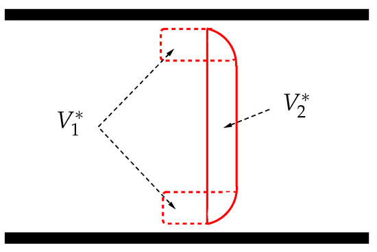
Figure 2.
Splitting the RBC volume into and .
The total volume can be calculated as , where , hence (in [5] is simply estimated as ).
Considering , we obtain if . Actually is not allowed to approach , otherwise the flow becomes impossible (see [4] for a discussion).
For instance, when , we get (in [5] , thus giving , if ). . The approximation is valid as long as , since on one side we have written , (RBC of cylindrical shape) but when the domain left is slightly smaller. Actually, since the RBC boundary is round there is some interval of values of R, before it reaches , in which , and we should simply replace with .
The length is a function of the hematocrit and is found by imposing the condition
Hence, from (1),
where b is given by (5) and
is a dimensionless constant (if, e.g., , then ). Note that b does not depend on . Moreover, the total length of a single element is
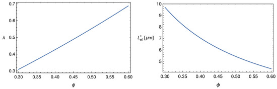
Now recalling (7), we introduce the dimensionless quantity
Figure 3 shows the behaviour of and versus .
If plasma filtrates through the vessel wall, the distance and the volume element will decrease in time. Thus, the element motion equation takes the following form
The expression for can be obtained as follows: compute the power dissipation in each stressed plasma layer for some translational velocity , imposing the no-slip condition at both layer boundaries, then write that the overall power dissipation equals the product . Omitting standard calculations (for more details we refer the readers to [5]), the result is
Hence, recalling (6), we rewrite (11) as
where we set , to put the equation in a form applicable to a continuum. This is justified by the fact that the number of elements in the capillary is sufficiently large ().
At this point it is convenient to recall the ratio that we are going to use as a fitting parameter (the only one in the model). With the help of it and recalling (12), we rewrite the expression of
which, being proportional to , has the character of a viscous force.
Concerning , we estimate it by considering a steady flow in typical conditions, imposing that the l.h.s. of (14) vanishes and taking the guess , to be verified a posteriori. This has been done in [5] obtaining
Let us now derive the dimensionless form of (14) recalling the characteristic transit time , and introducing the dimensionless variables , , , and
We recall that is and (if, e.g., ) we find . Thus, inertia has no role in (17). With the same value of we get , which confirms that the performed rescaling is suitable. Eventually, (17) reduces to
Now we shift our attention to the dynamics of plasma filtration through the capillary wall, in other words to the evolution of . On one side we have that no RBCs are loss during the flow, thus their concentration obeys the continuity equation
The plasma loss rate through the capillary wall is driven by the difference , being the external fluid pressure, and is opposed by the so called oncotic pressure resulting from the presence of proteins in plasma (mainly albumin), responsible for osmosis. Since the plasma volume fraction is , the plasma balance can be written as follows (Starling’s law)
where in the permeability of the capillary wall and is the oncotic pressure, a function of the total proteins concentration in blood , usually given in g/dL,
given by the Landis–Pappenhaimer formula (see [7], vol. 2, Chapt. 29). The three coefficients , , have the values reported in Table 1.

Table 1.
Values of the three coefficients in (21).
As plasma flows out, proteins keep concentrating, since the product remains constant
where the quantities on the r.h.s. are the ones in circulating blood, hence the values at the capillary inlet. Note that is deducible from (7) putting . Hence, considering as reference protein concentration, and introducing , (22) rewrites as (in [5], where the term b is neglected, )
Equation (19) is readily written in dimensionless form
In order to reduce (24) to a dimensionless form too, we define the dimensionless constants
Recalling (16) and (21), Equation (24) can be rewritten as
with given by (23). Thus, the model consists of solving the differential system (18), (25) and (27), for the determination of the unknowns , u and p.
The main physiological application refers to the steady flows. Eliminating time dependence is a great simplification. First, Equation (25) implies
where , is the dimensionless blood velocity at the capillary inlet. Assuming , then u can be seen as a function of
and so (27) rewrites as (here, and in the sequel, we have set ).
Hence, and are obtained solving this Cauchy for
where , and are given by (7), (10) and (23), respectively, and where, recalling (16),
, being the characteristic transmembrane pressure. In particular, following [8,9], we introduce the osmotic number
and, recalling (26), we rewrite (31) as
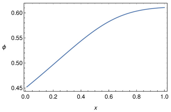
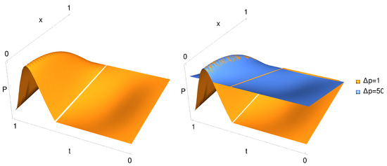
Figure 4.
Behaviour of for and , when .

Figure 5.
Behaviour of given by (29) for and , .
In [5], the steady-flow model (30) has been applied to the capillaries in the renal glomerulus obtaining the physiological value of the renal filtration rate. For more references and details, also on historical aspects, see [1].
Modeling the Flow through Fenestrated Capillaries: Conclusions
We have reviewed a model for blood flow in fenestrated capillaries based on an approach outside the standard fluid dynamical context. Indeed, the model considers the motion of plasma-RBC elements imposing the balance between the driving force produced by the hydraulic pressure gradient and the drag caused by friction at the vessel wall. The latter takes place in the thin plasma layer confined by the RBC portion facing the capillary wall (see Figure 1) and in a layer of the plasma segment between two consecutive RBCs in the flowing sequence. Plasma loss through fenestrations, altering the system configuration, is particularly intense in the highly fenestrated capillaries making the renal glomeruli, and is driven by the pressure across the vessel wall, which includes the effect of osmosis. Osmosis plays a fundamental role, since proteins (mainly albumin) in blood are not allowed to leave the capillary, whose wall behaves as a semi-permeable membrane. The progressive plasma loss increases the albumin concentration thus enhancing osmosis. The model has been applied in [5] to compute the glomerural filtration rate (i.e., the amount of the plasma filtrated by kidneys in one minute). The physiological value has been successfully retrieved.
3. Modeling Vasomotion
Rhythmic contractions of blood vessels equipped with smooth muscle are normally independent on heart pulsation or respiratory rhythm. This phenomenon, called vasomotion, is easily observed in the veins in the bat’s wing and was first noticed by T.W. Jones [10] in 1852. The biological mechanisms driving the onset of persisting oscillations have been studied in a number of papers, [11,12,13,14,15,16,17,18,19,20]. Vasomotion ordinary values for frequency and amplitude are 10 cpm and 25% of mean diameter, though values of 25 cpm and 100% are possible [21].
Literature on vasomotion physiology is rather numerous since one of the main concern is about its benefit to microcirculation. Indeed, vasomotion is particularly active at the level of microcirculation where vessels resistance becomes large. Jones, in their paper [10], conjectured that vasomotion reduces the vessel resistance thus favoring blood flow. However, vasomotion appears reduced during pregnancy [22]. On the other hand, unexpectedly, it is upregulated in hypertensive states like preeclampsia (pregnancy induced severe hypertension), while a decrease in vessels resistance is believed to be advantageous in pregnant mammals. Clearly, this does not help to clarify the role of this phenomenon.
The paper [23] takes a shortcut to show that vasomotion enhances flow in arteries, but their argument was pointed out to be incorrect in [24]. Experiments with bat wings (see [25]) suggest that venules vasomotion acts as a reciprocating pump, increasing blood flow rate, due to to valves preventing backflow. Indeed the phenomenon presents very different features in arterioles and in venules. The interaction flow-vasomotion is much more complicated in venules, because of the action of valves. The experiments illustrated in [25] show that pressure exhibits large peaks during the vessel contraction, which is compatible with the presence of an inlet and an outlet valve.
The whole matter of blood dynamics in the presence of vasomotion has been recently reconsidered in [24,26,27] (see [1] for a review). In [24] the authors make a clear distinction between the flow in the venules and in arterioles, while in [26,27] the effect of the presence of valves was investigated on the basis of a mathematical model with the aim of clarifying their real influence on blood flow. Comparing the model results with the experimental data by Dongaonkar et al. [25], it was concluded that in valves equipped venules, oscillations are converted in blood propulsion. On the contrary, in the valveless vessels (i.e., arterioles), vasomotion has little effect, and actually increases the hydraulic resistance thus reducing the flow rate, contrary to what was stated in [23].
In the paper [28] the case of vessels with distributed valves was considered, resulting in a model with a free boundary (the moving location of the engaged valve). The existence of distributed microvalves in venules has been reported in [29], where a condition of pressure continuity forces that value to remain between the imposed inlet and outlet values.
In this paper, we review the mathematical models for incompressible Newtonian flows in oscillating arterioles and venules. In our derivation we exploit the smallness of the ratio (we recall that the symbol “ ” denotes dimensional quantities).
where is the maximum vessel radius and is the vessel length.
Concerning arterioles, which are characterized by the absence of valves, in Section 3.1 we investigate the influence of vasomotion on the flow. Concerning venules, Section 3.2, the model requires to impose very peculiar boundary conditions (unilateral, or Signorini, boundary conditions), that take the valves action into account. We thus formulate a mathematical model for a peristaltic wave travelling along the vessel. In particular, denoting by the wavelength of the peristaltic oscillation, we investigate the flow analyzing two cases:
- , referred to as synchronous oscillation.
- , referred to as non synchronous oscillation.
The former consists of a uniform oscillation of the vessel walls, while in the second case a wave profile travels along the vessel.
The first case (synchronous oscillation) can, indeed, be recovered from the second one in the limit of “long” wavelengths, which guarantees the physical consistency of the model. In Section 3.8 we show numerical solutions that match the experimentally detected pressure behavior displayed in [25]. Since we are interested in the average flow, in the following we will systematically ignore pressure pulses by heartbeats, just considering the average hydraulic pressure gradient present in the studied vessels.
3.1. Vasomotion in Arterioles
We start considering vasomotion in arterioles, where usually ranges around , and model these vessels as cylindrical tubes. We denote by , and the longitudinal and radial coordinates and assume azimuthal symmetry so that the angular coordinate never appears and the velocity field is
We note that the muscle fibers surrounding the vessel can only contract and not dilate, so that the vessel radius is maximal in the rest configuration. Consequently the oscillation of the vessel wall causes a lumen narrowing. Hence we model the vessel oscillations as
where is the radius of the rest (undeformed) state, , and is the oscillations pulsation. Denoting by the time average over the period , we find . The periodic oscillations thus cause an average a reduction of the vessel lumen by .
Dealing with arterioles, where the flow is dominated by hydraulic pressure imposed by the heart, a natural scale for the longitudinal flow is
where , denotes the typical pressure drop and is the blood viscosity (typically ). If we take as approximate values , and , , it turns out that the formula above captures the correct magnitude order . In particular, exploiting (35) we can estimate the transit time as
getting . Hence, if the period of the walls oscillations is (which roughly corresponds to , i.e., ), we have
Concerning the characteristic radial velocity, we set
Taking , and a frequency of , we have , so that
Defining
and recalling (35) and (36), the dimensionless version of the Navier–Stokes and continuity equations is
where
We remark that the Reynolds number of the flow is rather small (less than 10), so that chaotic turbulence never occurs. At the leading order (40) reduces, as expected, to the classical Hagen–Poiseuille equation
Equation (41) implies that p is independent of r. while the continuity Equation (39) shows that is independent of x, so that p is linear in x. This fact fully justifies the shortcut adopted in [23] where the quasi steady Poiseuille discharge through the vessel is averaged over a period.
Denoting by the discharge
we find, after a little algebra, that the average discharge is
where
is the discharge corresponding to the radius at the rest state (in [23] the authors obtained a similar formula, but they compared the average flow rate with the one corresponding to the average vessel radius, which is not the rest state radius. Hence they erroneously concluded that vasomotion is advantageous for any amplitude), i.e., the undeformed configuration, and
In particular, since for , and when , we remark that is maximum for when . For any we have , so that vascular contractions due to vasomotor activity are disadvantageous for flow, at least in this simple framework. Indeed, the arteriole smooth muscle cells contract from a rest state corresponding to the maximum vessel size , and the lumen reduction can only hinder the flow. Thus, the question of the possible benefit of vasomotion in arterioles is left open and should be investigated in a scenario different from the one of a simple Newtonian flow in a vessel with synchronous oscillations.
The above analysis is correct within the order. Higher order approximations provide corrections not exceeding and are neglected.
3.2. Vasomotion in Venules
Because of the presence of valves which prevent backflow, vasomotion in venules produces a completely different effect. Indeed the pumping action generated by vasomotion on the flow is definitely comparable to the one due to the available pressure gradient.
Valves in the major veins had been observed since the early times of anatomy (see [1] at p. 60). On the contrary, the presence of valves in small veins has been underestimated or even ignored. An historical review on this subject is due to Caggiati et al. [29]. In particular, microscopic valves has been observed in venules as small as diameter, where they may be arranged in series (see [30,31]).
3.3. The Mathematical Model
We illustrate a model for venules equipped with just two valves placed at the inlet and outlet, corresponding to and . We attack the problem from a more general point of view, supposing that the vessel radius evolves as a travelling wave with wavelength , i.e.,
where:
- A.1
- is a periodic function (with period 1) such that , . Moreover we suppose that is decreasing in a fraction of the period (contraction phase) and increasing in the remaining fraction (expansion phase). Therefore, as in Section 3.1, the vessel radius in the natural undeformed state is (maximum cylinder lumen).
- A.2
- is a dimensionless parameter, so that , gives the oscillation amplitude (producing a lumen reduction with respect to the rest state).
- A.3
- is the wavelength and is the wave period, which are linked to the wave velocity by
We denote by the radial surface velocity. From (44)
where and where
represents the average contraction velocity, so that we replace (36) with . In vasomotion is available from experiments. Recalling the scaling (38), we introduce . We will focus on the following cases:
- much larger than (more precisely ), meaning that at the leading order the vessel undergoes spatially synchronous oscillations.
- comparable with , i.e., .
We do not consider the case , since in [32] we proved that in this case the peristalsis has basically no effect on the flow.
Differently from the case of arterioles, the pressure gradient in venules is low (few mmHg/mm) and we may assume that the flow is dominated by peristalsis. Therefore we choose the longitudinal reference velocity as follows
and set
so that . The reference pressure gradient is defined as
The quantity represents the order of magnitude of the “effective pressure drop” caused by the oscillations of the vessel (inspired to Poiseuille’s formula). The known imposed pressure difference is , and we consider
When , the flow is essentially dominated by the externally imposed pressure gradient and the effects due to the wall oscillations are hardly observable (which is exactly the case occurring in arterioles). We also introduce the dimensionless pressure
so that
We finally rescale the radial velocity of the vessel walls by , namely, by using (48),
3.4. Flow Equations
The line is a symmetry axis so that
The fluid mechanical incompressibility yields
and the motion equation reduces to Stokes equation
since the Reynolds number characterizing the flow is small (referring, for instance, to the data of [25] we have ). So (57) yields
which, at the leading order imply , and
Recalling boundary conditions (53) and (55), we find
with given by (48). We now insert (56) in (61), getting
Integrating between 0 and R and exploiting (54) we obtain
with u given by (52). The average longitudinal velocity is
The local dimensionless discharge at time t (within an approximation) is
corresponding to the physical quantity
3.5. Boundary Conditions at the Vessel Ends
The valves are placed at the vessels ends, and act to prevent backflow. Valves are considered as massless devices with a simple dynamics: when pressure exceeds the inlet one, the inlet valve closes; when pressure falls below the outlet one, the outlet valve closes. Let us express the corresponding boundary conditions. At , inlet valve, two conditions have to be fulfilled
The first condition simply states that backflow cannot occur (pressure is allowed to grow beyond when the valve is closed), while the second one guarantees that can never drop below the imposed pressure. Evidently, at least one of such conditions must be verified as an equality. As a consequence, the inlet boundary conditions summarize as follows
This is a typical unilateral boundary condition (also known as Signorini type condition) which is frequently encountered in continuum mechanics (see, for instance, [33]). Similarly, the boundary conditions at are
These conditions (graphically represented by the step functions, i.e., solid lines, in Figure 6) allow, as we shall see, to find an explicit formula for pressure and discharge. In this way the valves are modeled as massless devices which open/close instantaneously as the pressure in the vessel becomes larger/smaller than the one outside. Such an approach, though providing a significant agreement with the experiments reported in [25], have been improved in [27] where the valves inertia, which induces a delay in their action, has been considered.
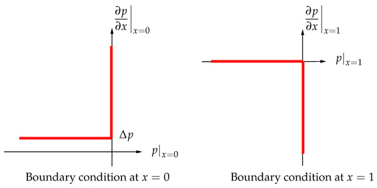
Figure 6.
Signorini type boundary conditions at and (pressure gradient vs. pressure).
3.6. Synchronous Oscillation:
This case essentially corresponds to a spatially uniform contraction/expansion of the vessel, i.e., . In particular, using the same notation of Formula (44), we take
with periodic function of period 1, and, recalling A.1 of Section 3.3, . Next, because of (52)
Functions , and are unknown and have to be determined. Condition (67) rewrites as
while (68) takes the form
We now assume the entrance valve engaged, that is , and consider the compression phase . From the first of (73)
which, exploiting (71), gives . Of course the third condition of (72) has to be fulfilled so that
On the other hand if
the entrance valve is open and the solution is
Hence, during the compression phase, i.e., , we have
In the expansion phase , we first consider
i.e., the exit valve is closed. The conclusion is that (the inlet dimensionless pressure). Then, recalling the third condition in (73), we notice that the compatibility condition (74) must once again be fulfilled. On the contrary, when condition (75) is fulfilled the exit valve is open and the condition yields
Summarizing, during the expansion phase, i.e., , the pressure is
We also observe that the flux has no interruption. Indeed, when a valve at one end is closed the one at the opposite end is open. Formula (63) allows to estimate the dimensionless discharge, which depends on the abscissa x along the vessel. In particular, when , we have (the case , has been extensively analyzed in [26]).
Therefore, during compression phase, i.e., when the inlet discharge vanishes, while in the expansion phase we have and the inlet flow rate becomes maximum. It is trivial to verify that the total inlet discharge equals the total output discharge. Moreover, the average flow in a period is not zero (as it would occur in absence of valves). Indeed, if a single oscillation over the period is considered, namely
the total volume (dimensionless) coming out of the vessel in a period (and which therefore enters the tube during the subsequent expansion phase) is
since, and . Hence, recalling (64), we have
that is the volume by which the cylinder is reduced during an oscillation.
The typical behavior of the outflux and influx, i.e., and , is displayed in Figure 7. The top panel shows the radius oscillation during a period (in this case ), while in the bottom panel and , given by (78). We remark that, during the compression phase, vanishes and since the outlet valve is open. During the expansion phase, , exactly the opposite occurs since the inlet valve is open.
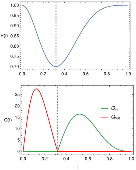
Figure 7.
Typical behaviour of , and .
3.7. Non-Synchronous Oscillation:
The case in which , i.e., non-synchronous oscillations, has been analyzed in detail in [26]. Here we recall briefly the main steps, considering, for the sake of simplicity, . Recalling (52) and (62), we write
which gives
where and are unknown at this stage.
We introduce
and define
Since conditions the third of both (67) and (68) are fulfilled, we need to prove only the second of (67) from which the second of (68) automatically follows because . Rewriting the second of (67) as
and using (82), we immediately obtain (81).
In order to highlight the difference between the two cases, we consider , which fulfils A.1, so that
Figure 8 displays the in influx, and the outflux , when is given by (83) with , and . In Figure 9 we still report and but in case of synchronous oscillations, i.e., when , with the same . The differences between the profiles reported in Figure 8 and Figure 9 are evident even if the flow rates peaks are the same. In case of synchronous oscillations, Figure 9, the two valves are never open at the same time and the inlet and outlet flow rates are symmetrical (because of to the peculiar behavior of ). In case of non-synchronous oscillations, i.e., Figure 8, there exists a time interval in which both valves are open. This is evidently attributable to the fact that the vessel contraction occurs as a traveling wave.
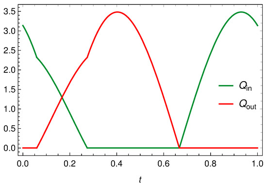
Figure 8.
Inlet and outlet discharge when is given by (83), with and .
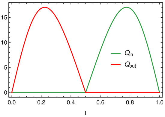
Figure 9.
Inlet and outlet discharge when with .
3.8. Model Validation
The comparison between the model and the experimental data by Dongaonkar et al. [25] has been discussed in details in [26,27].
We consider the experimental data reported in Figure 3 of [25], which represents the diameter oscillations of a bat wing venule. In particular, we select (recall that denotes the oscillation amplitude)
where we set , , , and .
The comparison between the experimental data of [25] (Figure 5, luminal pressure) and the pressure profile predicted by the model is shown in Figure 10. Considering the simplicity of the model (only two valves, inertia neglected, Newtonian context), the agreement appears rather satisfactory.
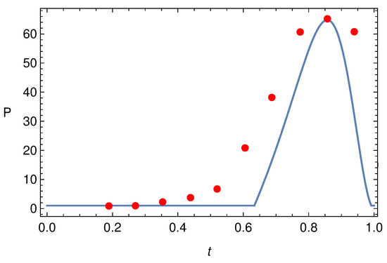
Figure 10.
Pressure pulse at when is given by (84) and the experimental data extracted from Figure 5 of [25].
3.9. Modeling Vasomotion: Conclusions
Periodic contraction-expansion of blood vessels have been recorded since 1852. Such phenomenon, usually referred to as vasomotion, concerns small (but not too small) vessels (arterioles and venules). The basic laws of fluid dynamics and the smallness of the radius/length ratio have been exploited to formulate a mathematical model which appears to be rather accurate.
First we have focused on arterioles, where the blood flow is essentially driven by hydraulic pressure gradient imposed by heart, concluding that the vessel resistance is increased by vasomotion. This is due to the lumen reduction caused by the vessel contraction (generated by the smooth muscle cells surrounding the arterioles) which actually hinders the flow. Actually such a result agrees with [22]: the resistance in a vessel with vasomotion is larger than the one of a static vessel with relaxed radius.
We then analyzed vasomotion in venules provided with just two compliant valves (one at the inlet and one at the outlet). We considered first the case of synchronous vessel oscillation. This can be seen as the limit of the peristaltic motion when the wavelength is much larger than the vessel length. The model has been tested versus the experimental measures by Dongaonkar et al. [25] performed on bat wing venules, which are characterized by periodic pressure pulses. Regardless of the simplicity of the model, the agreement obtained is remarkable. In particular, the model discussed in [27] which accounts effectively for valve inertia, reproduces the recorded pressure pulse almost perfectly. This suggests that the scheme with two valves provides a quite reasonable description of the phenomenon. On the contrary, the many valves model discussed in [28] produces a different qualitative behavior which is not compatible with the experimental measures of [25].
We have confined our analysis to the propulsive effect. In larger veins, valves exert a modulation effect that enhances the centripetal blood flow [34]. We finally emphasize that the two-valve model may be applicable to lymphagiones, the valves equipped elements making a lymphatic vessel.
4. The Fåhræus–Lindqvist Effect
The Fåhræus–Lindqvist (FL) effect is a phenomenon that occurs in blood vessels with diameter in the range and is named after the two Swedish scientists Robin Fåhræus and Johann Torsten Lindqvist [35]. It consists in a progressive reduction of the apparent blood viscosity as the blood vessel radius decreases. The FL effect is clearly related to the rheological properties of blood. Indeed, despite the blood composite nature, in tubes like veins and arteries above the size specified above and at relatively high shear rate (), this fluid shows the characteristic Newtonian behaviour of an incompressible liquid. At a smaller scale this is no longer true since inhomogeneity effects become highly significant and must be considered. Notwithstanding the great importance of this topic in physiology, until the fifties papers on blood rheology were scarce and not properly connected in textbooks or manuals dealing with blood or the blood circulation. Quoting Copley [36]
reviews on the viscosity of blood deal largely with data on apparent viscosities. The relative paucity of rheological treatments of blood is contrasted by the large number of observations of rheological phenomena of this humor.
Despite all the efforts and hundreds of studies devoted to the FL effect in the last ninety years, an explanation based on the principles of fluid dynamics has been achieved only very recently [37].
The physiologist and physicist Jean Poiseuille [38], in 1836, was the first to investigate the flow of human blood in narrow tubes. Experiments lead them to formulate their famous law that relates the fluid dynamic viscosity (as previously stated, starred quantities are dimensional) to the in-out pressure difference in the tube, the volumetric flux , and the tube length and radius , namely
Poiseuille experiments found their theoretical justification some years later, thanks to Navier and Stokes. Indeed, (85) can be proved to be a direct consequence of the Navier–Stokes equations of fluid mechanics. If blood is considered a homogeneous Newtonian fluid, then the stress and shear rate are directly proportional through a constant viscosity , which depends on temperature. In case of flow in a tube, Navier–Stokes equations can be solved explicitly for the velocity which shows a parabolic profile along a tube cross-section. Thus, being
the flow rate can be calculated by integrating , and (85) is theoretically justified.
What has all this to do with the FL effect? If blood were really Newtonian, its viscosity should not depend, in particular, on the tube radius. On the contrary Figure 12 shows that this is not true.
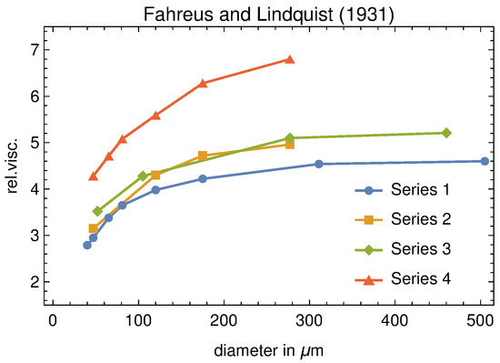
Figure 12.
Original data of the Fåhræus–Lindqvist experiment. The measured viscosity is relative to that of plasma. It should be emphasized that one of the blood samples (series 4) shows higher relative viscosity values than that the others, since was partially depleted of plasma by centrifugation.
Moreover, viscosity is measured at a given shear rate, an so, in principle, it could also depend on the latter. For a Newtonian fluid this ratio is a material constant which shows dependence only on temperature. Otherwise, viscosity is referred to with the name of “apparent” viscosity and denoted by . Figure 12 shows that blood turns from a Newtonian to a non-Newtonian behaviour as soon as the vessel diameter reduces below a threshold value.
The FL effect has an important physiological implication: the heart can drive a given volume of blood through the arterioles at a much lower pressure than would be the case if the blood were a Newtonian fluid.
The non-Newtonian behaviour of blood in small tubes has received several qualitative explanations, the most important one being related to the fact that blood is not a simple a liquid, but rather a non-homogeneous suspension of various particles. Among all these particles, RBCs contribute by far the highest percentage. In the next section we outline the Haynes’ conjecture, which was the first tentative to interpret the FL effect as a consequence of a “smart” response of the RBCs to the narrowing of the vessel diameter.
4.1. The Haynes’ Conjecture and Its Physiological Implications
According to Haynes [39], in vessels with diameter smaller than , RBCs tend to migrate towards the central part of the vessel, while a less viscous layer of plasma, named “marginal zone” or “cell-free layer” (CFL), forms close to the walls. The viscosity in the marginal zone is basically the one of the suspending liquid (plasma), denoted by . The viscosity of the RBCs suspension in the central core of the tube is assumed to be uniform and is denoted by . Haynes’ leading idea is that the presence of the marginal zone reduces the apparent viscosity in tubes of small diameter. This reminds Jeffery [40] who heuristically hypothesized that
Indeed, since the viscosity of the marginal layer is from 4 to 5 times less than that of the core, the wall stress is drastically reduced. In the Haynes’ view, the physiological motivation of the migration of the RBCs toward the center of the tube is to reduce the pumping effort of the heart. Recently, Ascolese et al. [41] showed that this heuristic explanation is misleading.the particles will tend to adopt that motion which, of all motions possible under the approximate equations, corresponds to the least dissipation of energy.
Following their approach, we first recall that blood is treated as an inhomogeneous incompressible linear viscous fluid, whose viscosity depends on the hematocrit . If is the velocity, the model equations are
where the differential operators are referred to dimensional variables, is the blood density, the pressure, and , with the hematocrit-dependent blood viscosity, and . Concerning , the current literature offers a variety of empirical laws (see, for example, [42,43,44,45,46,47]).
Although blood generally shows shear thinning and stress relaxation proprieties [1,48] these non-Newtonian effects can be neglected for the flow regimes and vessel sizes considered in [41].
Let us now specialize model (87) to the steady flow in a cylindrical tube whose diameter is and whose length is . If we denote by the radial coordinate, and suppose that the flow attains a steady laminar state
where is the unit vector parallel to the cylinder axis, the first two equations in (87) are identically satisfied, and the third reduces to
Equation (89) can solved for under standard (no-slip) boundary conditions:
and
where is the inlet hematocrit (usually between 0.35 and 0.5) and the in-out pressure difference.
According to Haynes’ conjecture, in vessels with diameter less than 0.3 mm, the RBCs migrate towards the center so that the flow region consists of an outer layer in which (also referred to as cell-free layer, CFL) and the complementary axisymmetric region to which all RBCs are segregated, where the hematocrit is constant and uniform. The two regions are separated by an interface with constant but unknown radius s. Therefore, is a stepwise function
and the flow has the so-called core-annulus structure (CAS). Since Equation (91) has to be fulfilled, s is not arbitrary. Although other choices of are possible (see, for example, Phillips et al. [49]), the advantage of (92) is that it allows to solve the flow problem explicitly.
The continuity of velocity and shear stress at the unknown interface s leads, after standard calculations, to obtain the velocity profile in the tube and to evaluate, consequently, the discharge: indeed
and
so that the total discharge is
The total power dissipation by the viscous friction along the tube is
while the total flow discharge for a given pressure drop is
Thus, by using (93), it follows
The key point is that can be expressed in the form , where
is the blood viscosity before entering the vessel, and is a dimensionless strictly decreasing function of whose explicit form depends on the way one chooses to evaluate as a function of the hematocrit. Ascolese et al. [41] evaluated for six different choices of and for four different values of (see Figure 6 in the cited paper). In all cases considered, for and as . Thus, (100) implies that increases as decreases, meaning greater dissipation when a CFL is present. At the same time increases above its value before entering the vessel, which in physiological terms means an increase of the perfusion effect towards the peripheral tissues. This conclusion elucidates, more than others, the crucial role of the FL effect in physiology.
Formula (97) follows almost directly from the Haynes’ conjecture and from the calculus of the total (core and plasma layer) discharge. Far from giving a justification of the CFL, its utility is confined to provide an estimate of (difficult to measure) as a function of the other, experimentally measurable, parameters, provided a reliable is given. However, two questions remain still unanswered: is a boundary layer already present also in “large” vessels? In the affirmative case, why the layer thickness increases when blood flows from a given vessel to a smaller one? The first question is usually explained in terms of the so-called size exclusion effect (see, for example [50,51,52]): RBCs cannot get close to the vessel wall for less than half of their minimal thickness (≈ 2–3). Thus, the CFL thickness cannot be lower than ≈ 1–1.5. The second question has been fully answered by Guadagni and Farina in [53] by applying the Prandtl boundary layer theory (see, for example, [54]). They show that the marginal layer, after an “entrance effect”, quickly reaches a steady value. The main contribution of that paper is to provide an exact relation which links the asymptotic thickness of the CFL to its initial (minimum) value dictated by the size exclusion effect. This is the key step towards a rigorous justification of the FL effect. In particular, in [37] we compared the marginal layer thickness, as predicted by the mathematical model, and some measured values taken from “in vivo” experiments by Maeda et al. [55] and by Kim et al. [56]. In all cases we obtained results that, considering the uncertainty due to the experimental errors, are quite satisfactory.
4.2. The CAF Evolution Explained as an Entrance Effect
In [53] the Authors, working in planar geometry, study the entrance effect. They show that the velocity has a transverse component which shifts streamlines towards the channel center and it is bound to vanish just beyond the entrance region. So the flow reaches very soon a stratified structure where the particle volume fraction close to the wall significantly lower than the one in the core. The proof is quite technical and cannot be reported here.
Here we partially extend the argument of [53] to cylindrical geometry. Furthermore, in this case, as expected, it turns out that flow soon reaches a CAF structure as the one hypothesised by Haynes [39].
Let us denote by the minimum size of the outer layer, i.e., , with . It is reasonable to guess that is going to depend on the geometrical properties of the RBCs in the considered sample, thus a quantity whose value cannot be given a priori with great accuracy, though its range is limited around the RBC average thickness. We now rewrite system (87) in dimensionless form by introducing the following new variables
where is the longitudinal length scale, is the constant and uniform suspension density, the characteristic inlet velocity, the plasma viscosity (taken as the reference one), and . Then, if is the Reynolds number, we define , meaning that the choice of defines the aspect ratio of the entrance region. We also denote by and the (dimensionless) core and marginal layer viscosities, respectively. Clearly, if the marginal layer is just pure plasma, then , but in Section 4.3 we will allow to deviate slightly away from unity.
Because of symmetry, , while , and all unknowns are independent of the angular coordinate. Next, we assume that can be used as a small parameter. Then, neglecting all terms , , system (87) in dimensionless form rewrites (in both layers)
where, of course, is the viscosity of the layer considered. The following inlet conditions are assumed:
with , constant and , where a is the inlet thickness of the marginal layer (according to the size exclusion effect). The interface between the core and the marginal layer is denoted by and given by
Since is a (steady) material surface, we have
and, consequently,
The whole problem consists in solving the following coupled systems of Prandtl equations
to which the following free boundary conditions need to be added
where denotes the jump through . System (103)–(105) allows an asymptotic solution of Poiseuille type for , namely and
where . Since is a material curve
Thus, the initial core radius and its asymptotic value are related through
We notice that (107) is a fourth order algebraic equation in the unknown , with only one physically significant solution i.e., ,
We notice that (108) is independent of . The behaviour of as a function of is shown in Figure 13. If we can solve system (103)–(105) in the whole region and and prove that decays rapidly to , then (108) can be used to verify the FL effect versus the experimental data.
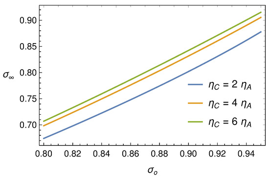
Figure 13.
Function (108) for some values of the ratio .
4.3. The Fåhræus–Lindqvist Effect Justified through Fluid Mechanics
In [53] Guadagni and Farina use the Langhaar’s approach [57] to solve the boundary layer equation in plane geometry. In the tube geometry a similar argument can be developed (see, for example, Sparrow et al. [58], Avula [59], Gupta [60] and Campbell and Slattery [61]).
We confine ourselves to summarize the guidelines of the procedure and report the evolution of for various choices of the relevant parameters.
It is well-known that it is not possible to solve Prandtl’s equations explicitly, so that special approximating techniques are needed. Here, the method consists in linearizing the inertia terms in the second of (103) and (104), in order to transform the momentum equation in the form
where and are auxiliary functions still to be specified. Imposing the boundary condition , the solution to (109) can be expressed as
where and are Bessel functions of the first modified and second type, respectively, and has to be determined. The same argument applies to the inner layer and, by imposing the boundary condition , one obtains
where , as well as , have to be determined. If we insert (111) and (110) into the second of (105) and the third of (105), we get an algebraic system that allows to express and in terms of C and D. Substituting again into (111) and (110), entails
where
and
is the regularized hyper-geometric function (from now on, we do not report the explicit expressions of the involved functions (which are, indeed, exceedingly long to be shown) and focus on the procedure).
To make the solution physically consistent we need to impose both the momentum balance and mass conservation (which, otherwise, may not be satisfied by the approximate solution), i.e.,
Now, by inserting (112) into the second of (117), we determine and . For to be consistent with the asymptotic solution (106), must vanish as . This can be achieved by expanding (112) for (that is for ) and verifying that at the zeroth order in , identifies with given by (106). At this point, the final step is to obtain two equations for and . The former follows by applying the second of (117) once again, in which is computed through the second of (103), evaluated at . The latter follows by the kinematic condition (105). Finally we have to solve a system of two ODEs of type
to be coupled with “suitable” initial conditions (in the sense specified in [53]), one of them being . Figure 14, Figure 15 and Figure 16 show, each for a given , the solution for and for five values of the ratio .
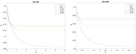
Figure 14.
The evolution of for , (left panel), and (right panel), and for some values of the ratio .
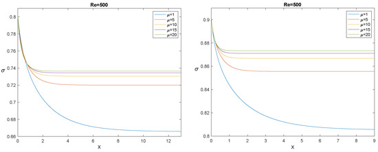
Figure 15.
The evolution of for , (left panel), and (right panel), and for some values of the ratio .
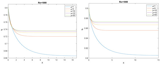
Figure 16.
The evolution of for , (left panel), and (right panel), and some values of the ratio .
The longitudinal interval needed by to decrease from to its asymptotic value is usually referred to as the “entrance length”. The most evident effect outlined by Figure 14, Figure 15 and Figure 16 is that, for fixed , the entrance length increases by increasing , while for any given , it decreases significantly by increasing . It must also be emphasized that simulations confirm that the asymptotic value depends only on , not on , as it must be, according to (108). In the next section, we compare the model with the experiments: in all cases we considered, the entrance length is rather small.
4.4. The Mathematical Model versus the Experimental Data
Now, as in [37], we use formula (108), where
and is a fitting parameter. Physically, this means that we consider the marginal layer not completely free of RBCs. A reasonable explanation may be that the “marginal exclusion effect” cannot be precisely stated (as it would be if the RBCs were rigid spheres) and it should be more understood as a statistical concept (see, for example, Ethier and Simmons, 2007). Thus, it is acceptable to think that a small percentage of hematocrit is present in the marginal layer and that this value may have some variability (Kim et al., 2007 refer to the outer layer also as a “cell–poor” region).
Now we can combine Formulas (108) and (119) with , where and a (the minimum outer thickness) is a fitting parameter related to the half thickness of the RBCs, so with a limited range of variability, i.e., 1–1.5 , since the average RBCs thickness is about 2–3 (see [62]). The result is a dimensional formula for the core radius s as a function of the tube diameter D, namely
where, however, are “tuning” parameters with very little variability.
Figure 17 shows how the mathematical model fits the original data. The fits by means of two popular empirical formulas are also shown for comparison.
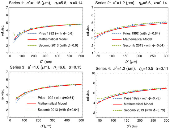
Figure 17.
Comparison between the experimental series 1, 2, 3 and 4 reported in Tables at page 565 of Fåhræus and Lindqvist [35] (dots) and the theoretical model (solid curve). The fitting via the empirical formulas by Pries [63] and by Secomb [64] are also shown (dashed curves). On the top of each plot the values of , , and the hematocrit used in the empirical formulas to fit the Fåhræus and Lindqvist data.
The model has been tested versus other classical experiments like those by Kümin [65] and by Zilow and Linderkamp [66]. Figure 18 and Figure 19 show that the agreement is at least as good as the empirical formulas also in these cases.
Figure 18.
Comparison between our model and the experimental data by Kümin [65] (dots). Data are extracted from Figure 2, at p. 1195 of [39]. The empirical fitting via the empirical formulas by Pries and by Secomb are also shown (dashed curves).
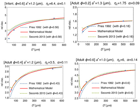
Figure 19.
Comparison between our mathematical model (solid curve) and data by Zilow and Linderkamp [66] (dots). These authors considered both adult and infant blood samples at different values of the hematocrit. The empirical fitting via the empirical formulas by Pries and by Secomb are also shown (dashed curves).
4.5. The Fåhræus–Lindqvist Effect: Conclusions
Starting form the seminal work of Fåhræus and Lindqvist [35], we recalled the relevance of the Haynes’ conjecture [39] in suggesting the right path to follow for a rigorous justification of the FL effect based on fundamental principles of fluid dynamics. Then we showed that this goal is achieved by relating the two recent contributions by Ascolese et al. [41] and Guadagni and Farina [53], thus solving a problem remained open for more than ninety years. To this end, the theory developed in [53] for flows in a plane symmetry has been here updated to the the case of axisymmetric flows. This relation contains, as a parameter, only the ratio between the viscosity of outer and inner layers. Finally, following [37], we showed how this formula can be used to fit, quite reasonably, not only the original data by Fåhræus–Lindqvist, but also those of other classical experiments Zilow and Linderkamp [66], by Kümin [65], and even two well-known empirical formulas proposed by Pries [63] and Secomb [64].
Author Contributions
The authors equally contributed to this article. All authors have read and agreed to the published version of the manuscript.
Funding
This research received no external funding.
Conflicts of Interest
The authors declare no conflict of interest.
References
- Fasano, A.; Sequeira, A. Hemomath: The Mathematics of Blood; Springer: Berlin/Heidelberg, Germany, 2017. [Google Scholar]
- Robertson, A.; Sequeira, A.; Kameneva, M. Hemorheology. In Hemodynamical Flows: Modeling, Analysis and Simulation; Oberwolfach Seminars; Birkhäuser: Basel, Switzerland, 2008; Volume 37, pp. 63–120. [Google Scholar]
- Robertson, A.; Sequeira, A.; Owens, R. Cardiovascular Mathematics. Modeling and Simulation of the Circulatory System. In Hemorheology; Springer: Berlin, Germany, 2009; pp. 211–242. [Google Scholar]
- Pozrikidis, C. Axisymmetric motion of a file of red blood cells through capillaries. Phys. Fluids 2005, 17, 645–657. [Google Scholar] [CrossRef]
- Farina, A.; Fasano, A.; Mizerski, J. A new model for blood flow in fenestrated capillaries with application to ultrafiltration in kidney glomeruli. Adv. Math. Sci. Appl. 2013, 23, 319–337. [Google Scholar]
- Remuzzi, A.; Brenner, B.; Pata, V.; Tebaldi, G.; Mariano, R.; Belloro, A.; Remuzzi, G. Three-dimensional reconstructed glomerular capillary network: Blood flow distribution and local filtration. Am. J. Physiol. 1992, 263, F562–F572. [Google Scholar] [CrossRef] [PubMed]
- Landis, E.; Pappenheimer, J. Exchange of substances through the capillary walls. In Handbook of Physiology. Circulation; American Physiological Society: Washington, DC, USA, 1963; Chapter 29; pp. 961–1034. [Google Scholar]
- Borsi, I.; Farina, A.; Fasano, A. The effect of osmotic pressure on the flow of solutions through semi-permeable hollow fibers. Appl. Math. Model. 2013, 37, 5814–5827. [Google Scholar] [CrossRef]
- Ronco, C.; Garzotto, F.; Kim, J.C.; Fasano, A.; Borsi, I.; Farina, A. Modeling blood filtration in hollow fibers dialyzers coupled with patient’s body dynamics. Rend. Lincei Mat. Appl. 2016, 27, 369–412. [Google Scholar] [CrossRef]
- Jones, T.W. Discovery that veins of the bat’s wing (which are furnished with valves) are endowed with rhythmical contractility and that the onward flow of blood is accelerated by each contraction. Philos. Trans. R. Soc. Lond. 1852, 142, 131–136. [Google Scholar]
- Reho, J.J.; Zheng, X.; Fisher, S.A. Smooth muscle contractile diversity in the control of regional circulations. Am. J. Physiol. Heart Circ. Physiol. 2014, 306, H163–H172. [Google Scholar] [CrossRef]
- Haddock, R.E.; Hill, C.E. Rhythmicity in arterial smooth muscle. J. Physiol. 2005, 566, 645–656. [Google Scholar] [CrossRef]
- Aalkjæ r, C.; Nilsson, H. Vasomotion: Cellular background for the oscillator and for the synchronization of smooth muscle cells. Br. J. Pharmacol. 2005, 144, 605–616. [Google Scholar] [CrossRef] [PubMed]
- Parthimos, D.; Haddock, R.E.; Hill, C.E.; Griffith, T.M. Dynamics of a three-variable nonlinear model of vasomotion: Comparison of theory and experiment. Biophys. J. 2007, 93, 1534–1556. [Google Scholar] [CrossRef] [PubMed]
- Ursino, M.; Fabbri, G.; Belardinelli, E. A mathematical analysis of vasomotion in the peripheral vascular bed. Cardioscience 1992, 3, 13–25. [Google Scholar] [PubMed]
- Matchkov, V.V.; Gustafsson, H.; Rahman, A.; Boedtkjer, D.M.; Gorintin, S.; Hansen, A.K.; Bouzinova, E.V.; Praetoriu, H.A.; Aalkjaer, C.; Nilsson, H. Interaction between Na/K pump and Na/Ca2 exchanger modulates intercellular communication. Circ. Res. 2007, 100, 1026–1035. [Google Scholar] [CrossRef] [PubMed]
- de Wit, C. Closing the gap at hot spots. Circ. Res. 2007, 100, 931–933. [Google Scholar] [CrossRef]
- Haddock, R.E.; Hirst, G.D.S.; Hill, C.E. Voltage independence of vasomotion in isolated irideal arterioles of the rat. J. Physiol. 2002, 540, 219–229. [Google Scholar] [CrossRef] [PubMed]
- Rivadulla, C.; de Labra, C.; Grieve, K.L.; Cudeiro, J. Vasomotion and neurovascular coupling in the visual thalamus. PLoS ONE 2011, 6, e28746. [Google Scholar] [CrossRef] [PubMed]
- Koenigsberger, M.; Sauser, R.; Bény, J.L.; Meister, J.J. Effects of arterial wall stress on vasomotion. Biophys. J. 2006, 91, 1663–1674. [Google Scholar] [CrossRef]
- Intaglietta, M. Vasomotion and flowmotion: Physiological mechanisms and clinical evidence. Vasc. Med. Rev. 1990, 2, 1101–1112. [Google Scholar] [CrossRef]
- Gratton, R.J.; Gandley, R.E.; McCarthy, J.F.; Michaluk, W.K.; Slinker, B.K.; McLaughlin, M.K. Contribution of vasomotion to vascular resistance: A comparison of arteries from virgin and pregnant rats. J. Appl. Physiol. 1998, 85, 2255–2260. [Google Scholar] [CrossRef] [PubMed]
- Meyer, C.; de Vries, G.; Davidge, S.T.; Mayes, D.C. Reassessing the mathematical modeling of the contribution of vasomotion to vascular resistance. J. Appl. Physiol. 2002, 92, 888–889. [Google Scholar] [CrossRef]
- Fasano, A.; Farina, A.; Caggiati, A. Modeling vasomotion. Rev. Vasc. Med. 2016, 8, 1–4. [Google Scholar] [CrossRef]
- Dongaonkar, R.M.; Quick, C.M.; Vo, J.C.; Meisner, J.K.; Laine, G.A.; Davis, M.J.; Stewart, R.H. Blood flow augmentation by intrinsic venular contraction. Am. J. Physiol. Regul. Integr. Comp. Physiol. 2012, 302, R1436–R1442. [Google Scholar] [CrossRef]
- Farina, A.; Fusi, L.; Fasano, A.; Ceretani, A.; Rosso, F. Modeling peristaltic flow in vessels equipped with valves: Implications for vasomotion in bat wing venules. Int. J. Eng. Sci. 2016, 107, 1–12. [Google Scholar] [CrossRef]
- Cardini, M.; Farina, A.; Fasano, A.; Caggiati, A. Blood flow in venules: A mathematical model including valves inertia. Veins Lymphat. 2019, 8, 7946. [Google Scholar] [CrossRef]
- Farina, A.; Fasano, A. Incompressible flows through slender oscillating vessels provided with distributed valves. Adv. Math. Sci. Appl. 2016, 25, 33–42. [Google Scholar]
- Caggiati, A.; Phillips, M.; Lametschwandtner, A.; Allegra, C. Valves in small veins and venules. Eur. J. Vasc. Endovasc. Surg. 2006, 32, 447–452. [Google Scholar] [CrossRef] [PubMed]
- Caggiati, A.; Bertocchi, P. Regarding “Fact and fiction surrounding the discovery of the venous valves”. J. Vasc. Surg. 2001, 33, 1317. [Google Scholar] [CrossRef] [PubMed][Green Version]
- Caggiati, A. The venous valves in the lower limbs. Phlebolymphology 2013, 20, 87–95. [Google Scholar]
- Fusi, L.; Farina, A.; Fasano, A. Short and long wave peristaltic flow: Modeling and mathematical analysis. Int. J. Appl. Mech. 2015. [Google Scholar] [CrossRef]
- Kikuchi, N.; Oden, J.T. Contact Problem in Elasticity: A Study of Variational Inequalities and Finite Element Methods; SIAM: Philadelphia, PA, USA, 1988. [Google Scholar]
- Lurie, F.; Kistner, R.L. The relative position of paired valves at venous junctions suggests their role in modulating three-dimensional flow pattern in veins. Eur. J. Vasc. Endovasc. Surg. 2012, 337–340. [Google Scholar] [CrossRef] [PubMed]
- Fåhræus, R.; Lindqvist, T. The Viscosity Of The Blood In Narrow Capillary Tubes. Am. J. Physiol. 1931, 96, 562–568. [Google Scholar] [CrossRef]
- Copley, A.L. The rheology of blood. A survey. J. Colloid Sci. 1952, 7, 323–333. [Google Scholar] [CrossRef]
- Farina, A.; Rosso, F.; Fasano, A. A Continuum Mechanics Model for the Fåhræus-Lindqvist Effect. J. Biol. Phys. 2021. [Google Scholar] [CrossRef]
- Poiseuille, J.L.M. Observations of blood flow. Ann. Sci. Nat. 1836, 5, 111–115. [Google Scholar]
- Haynes, R.F. Physical Basis of the Dependence of Blood Viscosity on Tube Radius. Am. J. Physiol. 1960, 198, 1193–1200. [Google Scholar] [CrossRef]
- Jeffery, G.B. The motion of ellipsoidal particles immersed in a viscous fluid. Proc. Ray. Soc. 1922, 102, 161–179. [Google Scholar]
- Ascolese, M.; Farina, A.; Fasano, A. The Fåhræus-Lindqvist effect in small blood vessels: How does it help the heart? J. Biol. Phys. 2019, 45, 379–394. [Google Scholar] [CrossRef]
- Nubar, Y. Effect of slip on the rheology of a composite fluid: Application to blood. Biorheology 1967, 4, 113–117. [Google Scholar] [CrossRef] [PubMed]
- Krieger, I.M.; Dougherty, T.J. A mechanism for non-Newtonian flow in suspensions of rigid spheres. Trans. Soc. Rheol. 1959, 3, 137–152. [Google Scholar] [CrossRef]
- Bingham, E.C.; White, G.F.; Amer, J. The viscosity and fluidity of emulsions, crystalline liquids and colloidal solutions. Chem. Soc. 1911, 33, 1257–1275. [Google Scholar] [CrossRef]
- Charm, S.E.; Kurland, G.S. Blood Flow and Microcirculation; John Wiley: Hoboken, NJ, USA, 1974. [Google Scholar]
- Cokelet, G.R. The Rheology of Human Blood. Ph.D. Thesis, MIT, Cambridge, MA, USA, 1963. [Google Scholar]
- Hatschek, E. Eine Reihe von abnormen Liesegang’schen Schichtungen. Colloid Polym. Sci. 1920, 27, 225–229. [Google Scholar] [CrossRef]
- Yeleswarapu, K.K.; Kameneva, M.V.; Rajagopal, K.R.; Antaki, J.F. The flow of blood in tubes: Theory and experiment. Mech. Res. Commun. 1998, 25, 257–262. [Google Scholar] [CrossRef]
- Phillips, R.; Armstrong, R.; Brown, R.; Graham, A.; Abbott, J. A Constitutive Equation for Concentrated Suspensions That Accounts for Shear-induced Particle Migration. Phys. Fluids 1992, 4, 30–40. [Google Scholar] [CrossRef]
- Secomb, T.W. Blood Flow in the Microcirculation. Annu. Rev. Fluid Mech. 2017, 49, 443–461. [Google Scholar] [CrossRef]
- Ethier, R.C.; Simmons, C.A. Introductory Biomechanic; Cambridge University Press: Cambridge, UK, 2007. [Google Scholar]
- Roselli, R.J.; Diller, K.R. Biotransport: Principles and Applications; Springer: Berlin/Heidelberg, Germany, 2011. [Google Scholar]
- Guadagni, S.; Farina, A. Entrance flow of a suspension and particles migration towards the vessel center. Int. J. Nonlinear Mech. 2020, 126, 103587. [Google Scholar] [CrossRef]
- Schlichting, H.; Gersten, K. Boundary-Layer Theory; Springer: Berlin/Heidelberg, Germany, 2017. [Google Scholar]
- Maeda, N.; Suzuki, Y.; Tanaka, S.; Tateishi, N. Erythrocyte flow and elasticity of microvessels evaluated by marginal cell-free layer and flow resistance. Am. J. Physiol. Heart Circ. Physiol. 1996, 271, H2454–H2461. [Google Scholar] [CrossRef] [PubMed]
- Kim, S.; Kong, L.R.; Popel, A.S.; Intaglietta, M.; Johnson, P.C. Temporal and spatial variations of cell-free layer width in arterioles. Am. J. Physiol. Heart Circ. Physiol. 2007, 293, H1526–H1535. [Google Scholar] [CrossRef]
- Langhaar, H.L. Steady flow in the transitional length of a straight tube. J. Appl. Mech. 1942, 64, A55–A58. [Google Scholar] [CrossRef]
- Sparrow, E.M.; Lin, S.H.; Lundgren, T.S. Flow developents in the hydrodynamic entrance region of tubes and ducts. Phys. Fluids 1964, 7, 338–347. [Google Scholar] [CrossRef]
- Avula, X.J.R. Analysis of suddenly started laminar flow in the entrance region of a circular tube. Appl. Sci. Res. 1969, 21, 248–259. [Google Scholar] [CrossRef]
- Gupta, R.C. Laminar flow in the entrance of a tube. Appl. Sci. Res. 1977, 33, 1–10. [Google Scholar] [CrossRef]
- Campbell, W.D.; Slattery, J.C. Flow in the entrance of a tube. J. Basic Eng. 1963, 81, 41–45. [Google Scholar] [CrossRef]
- Fung, Y.C. Biomechanics: Mechanical Properties of Living Tissues; Springer: New York, NY, USA, 1981. [Google Scholar]
- Pries, A.R.; Neuhaus, D.; Gaehtgens, P. Blood viscosity in tube flow: Dependence on diameter and hematocrit. Am. J. Physiol. 1992, 263, 1770–1778. [Google Scholar] [CrossRef]
- Secomb, T.W.; Pries, A.R. Blood viscosity in microvessels: Experiment and theory. Comptes Rendus Phys. 2013, 14, 470–478. [Google Scholar] [CrossRef]
- Kümin, K. Bestimmung de Zähigkeitskoeffizienten für Rindeblut bei Newtonscher Strömung in Verschiden Weiten Röhren und Capillaren bei Physiologischer Temperatur. Ph.D. Thesis, Universität Bern, Friborg, Switzerland, 1949. [Google Scholar]
- Zilow, E.P.; Linderkamp, O. Viscosity Reduction of Red Blood Cells from Preterm and Full-Term Neonates and Adults in Narrow Tubes (Fåhræus-Lindqvist effect). Pediatr. Res. 1989, 25, 595–599. [Google Scholar] [CrossRef] [PubMed]
Publisher’s Note: MDPI stays neutral with regard to jurisdictional claims in published maps and institutional affiliations. |
© 2021 by the authors. Licensee MDPI, Basel, Switzerland. This article is an open access article distributed under the terms and conditions of the Creative Commons Attribution (CC BY) license (https://creativecommons.org/licenses/by/4.0/).