Novel Approach for EEG Signal Analysis in a Multifractal Paradigm of Motions. Epileptic and Eclamptic Seizures as Scale Transitions

Abstract

Two different operational procedures are proposed for evaluating and predicting the onset of epileptic and eclamptic seizures. The first procedure analyzes the electrical activity of the brain (EEG signals) using nonlinear dynamic methods (the time variations of the standard deviation, the variance, the skewness and the kurtosis; the evolution in time of the spatial–temporal entropy; the variations of the Lyapunov coefficients, etc.). The second operational procedure reconstructs any type of EEG signal through harmonic mappings from the usual space to the hyperbolic one using the time homographic invariance of a multifractal-type Schrödinger equation in the framework of the scale relativity theory (i.e., in a multifractal paradigm of motions). More precisely, the explicit differential descriptions of the brain activity in the form of 2 × 2 matrices with real elements disclose, through the in-phase coherences at various scale resolutions (i.e., as scale transitions), the multitude of brain neuronal dynamics, especially sequences of epileptic and eclamptic seizures. These two operational procedures are not mutually exclusive, but rather become complementary, offering valuable information concerning epileptic and eclamptic seizures. In such context, the prediction of epileptic and eclamptic seizures becomes fundamental for patients not responding to medical treatment and also presenting an increased rate of seizure recurrence.

1. Introduction

Epilepsy represents a chronic brain pathology with different etiologies, in which repeated seizures appear more than 24 h apart due to an excessive neuronal discharge or synchronic neuronal hyperexcitability. The pathogenesis of epilepsy includes around 1000 genes that can be involved, the imbalance between mediated inhibition of γ-aminobutyric acid (GABA) and mediated excitation of glutamate, the link between neurotransmitters and drug abuse and other specific pathophysiologic drawbacks linking to epilepsy at different levels of brain functionality. Epilepsy can be further arranged into focal, general or unknown onset. The diagnosis of epileptic seizures is suggested by a patient‘s history, family declarations, and semiology of epileptic seizures. Electroencephalogram (EEG) represents the primary tool for epilepsy, which helps classify the seizures between focal or generalized and can bring important information regarding epileptic syndrome features described by the patient. Video-EEG monitoring can confirm the type of the seizure and contribute to localizing the epileptogenic zone when neuroimaging is normal and surgery is a treatment option. Magnetic resonance imaging (MRI) helps in finding the etiology and allows the patient‘s evaluation before surgical treatment. It is commonly employed in focal epilepsy assessment under specific protocols that consider the clinical onset and EEG findings [1]. Genetic testing by microarray analysis, single-gene testing, karyotyping, gene panel testing, whole genome sequencing, and whole exome sequences raise the probability of finding epileptic causes but present low availability and high costs [2]. Epilepsy is a common neurological condition, affecting patients of all ages, having a negative impact on social life, health, behavior and economic factors for the patient and their family. Treatments offer a normal life for most patients but about 20–30% of them are non-responsive to conventional anti-epileptic drugs [1].

Various situations have been suggested as primary or secondary causes in epilepsy onsets. Out of all the causes we can name brain damage, foreign-body swallowing, drowning or infection of the central nervous system. The onset of epilepsy can occur for a normal healthy child with no other risk factors associated. Due to this, various prevention and control measures have been developed especially for secondary factors that may lead to epilepsy development [3]. Epilepsy does not have a known cure, but seizures can be controlled with medication in about 70% of cases. In the cases where seizures do not respond to medication, surgery, neurostimulation or dietary changes may be considered.

In the case of epileptic seizures, due to structural or functional problems in the brain, a group of neurons discharges in an abnormal, excessive and synchronized manner. Seizure prediction can play a particularly important role and refers to the attempt to predict epilepsy seizures based on EEG. The aim of a significant volume from the literature, as is the aim of the present paper, is to develop ”procedures” through which not only the prediction but also the type of epilepsy can be established. Although the first electroencephalograms (EEGs) were recorded 143 years ago, progress in interpreting them is extremely slow. As of now, there is no classification of the structures that appear in an EEG, nor is there a correspondence between these features and the activity of the brain.

Let us consider a particular pathology: the tonico-clonico seizure also known as eclampsia. Eclampsia represents a medical emergency during pregnancy, being associated with increased morbidity and mortality for both mother and child. Pregnancy hypertensive disorders, such as chronic hypertension and gestational hypertension, represent primary criteria for eclamptic seizure onset. The mechanism beyond this pathology refers to endothelial damage, during the abnormal placentation in the first trimester, which leads to abnormal blood supply with high arterial resistance and vasoconstriction. Following this mechanism, increased levels of cytokines and free radicals are released and determine endothelial damage at the uterine and cerebral sites, accompanied by neurological disorders. Eclampsia is characterized by generalized tonico-clonic seizures in women with preeclampsia and may occur during antepartum, intrapartum or postpartum periods. The prevention of maternal complications in patients with preeclampsia represents fetus and placenta delivery. The delivery time is decided according to clinical evaluation and gestational age. Common neurologic symptoms like headache or changes in visual functions may reflect brain impairment. EEG may detect brain damage before symptoms appear and before ischemic conditions may determine irreversible brain dysfunction. The prediction of eclamptic seizures using artificial intelligence may improve maternal and fetal outcomes, offering extra time for case management [4].

The clinical interpretation of electroencephalograms is mainly performed by visual recognition of certain structures and by associations made by the specialist physician [5]. The Fourier analysis cannot be applied because the signals associated with the electroencephalograms are not stationary. The signals are extremely weak, in the domain of microvolts, and are “submerged in high noise” [6]. For this reason, special attention must be paid to the quality of the electrodes used and their positioning. In addition, the identification and analysis of artifacts should not be underestimated, as they may occur due to slight movements of the electrodes, or contraction of the muscles below the electrodes.

In the present paper, two complementary operational procedures are proposed for evaluating and predicting the onset of epileptic and eclamptic seizures. The first procedure analyzes the electrical activity of the brain (EEG signals) using nonlinear dynamic methods, while the second one reconstructs any type of EEG signal based on the scale relativity theory (SRT). An approach based on the fractal paradigm within the SRT is presented here for the first time.

2. Analysis of Epileptic and Eclamptic Seizures by Applying Non-Linear Dynamics Methods

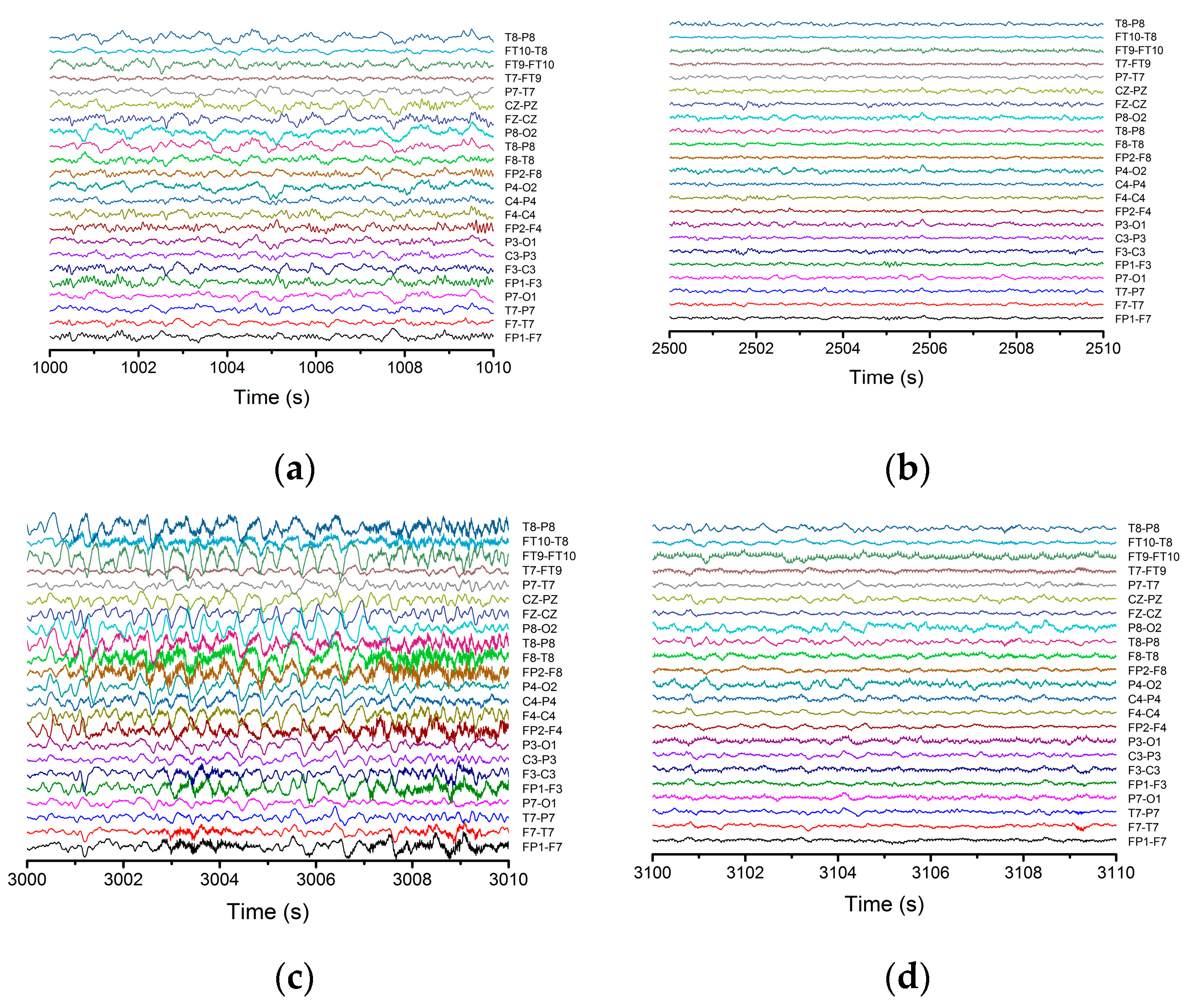
In this work the analyzed EEG signals were taken from the Physionet database. The data used corresponds to an epileptic patient aged 11 years on which we employed statistical and nonlinear procedures (standard deviation and variance, spatial–temporal entropy, Lyapunov exponents, etc.). The signals were collected on 23 channels with 16-bit resolution of each signal and a sampling time of 4 ms. The overall duration of the signal was 60 min while the duration of the epileptic seizure was of 40 s.

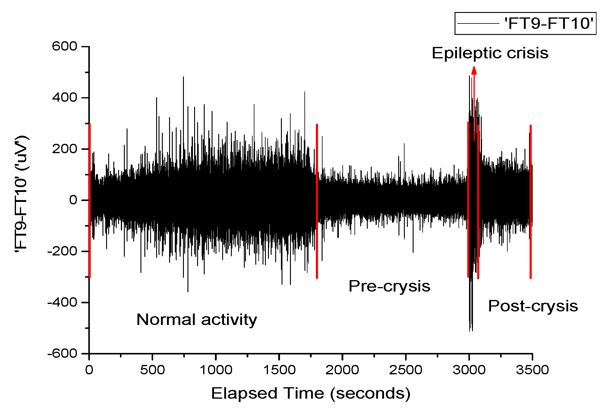
Figure 1 depicts the signal recorded on channel FP9-F10. It can be observed that neuronal activity does not have regular dynamics. The brain’s operating period can be divided into four areas of interest. The normal activity area of the brain (range 0–1800 s) is characterized by a chaotic dynamic, with a relatively high signal amplitude. The pre-epilepsy area (range 1800–3000 s) is characterized by a decrease in signal amplitude. In the epileptic seizure situs (range 3000–3040 s), the amplitude of the signal reaches its maximum value in a very short period of time, having more regular behavior due to the synchronization of the neurons’ activity. Lastly, the post-seizure zone (range 3040–3600 s) is where the signal amplitude decreases to a relatively small value but increases to the value corresponding to the area of normal neuronal activity.

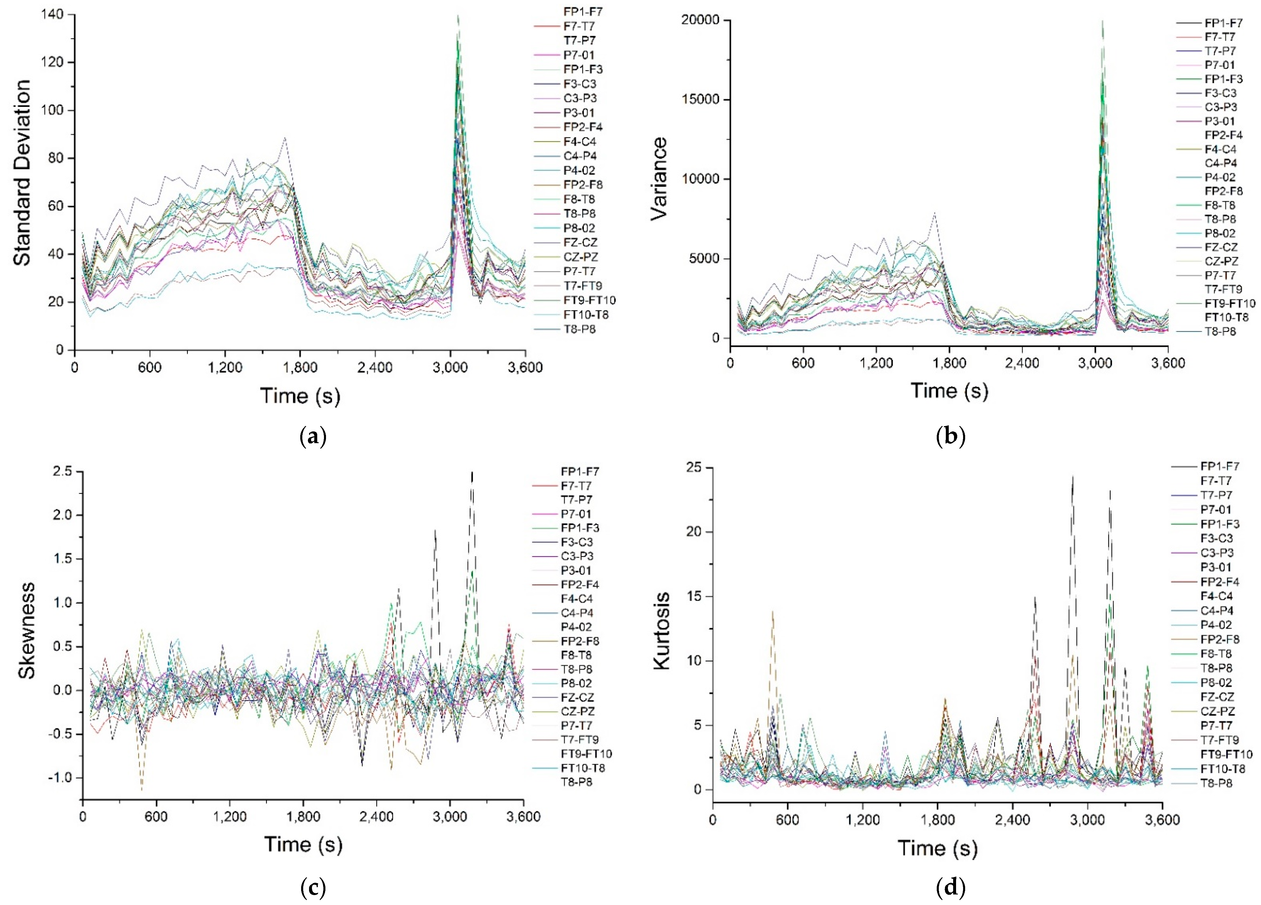
Neuronal activity (sequences of epileptic seizure) highlighted during the EEG signal from Figure 1, in the form of normal functioning of the brain, pre-epileptic seizure, epileptic seizure and post-seizure periods, are presented in Appendix A. The corresponding signals were analyzed with a series of statistical and nonlinear dynamics methods and only those results that allowed us to extract some information of interest are described. The graphical representation of the standard deviation (Figure 2a) shows that, before the pre-seizure, its value drops sharply (approximately until second 1800) and remains approximately constant until near the seizure (second 3000). During the epileptic seizure, the standard deviation presents an accentuated maximum. Since the standard deviation is an indicator of data dispersion, the fact that it remains at a small, approximately constant value during the pre-seizure period denotes that the recorded potentials have small, relatively equal values, so the nerve impulses at the neuron level are of small amplitude and have a “quiet” dynamic. During the seizure the values of the potentials deviate strongly from the average value. The same result, but much better outlined, is obtained from the graphical representation of the variance in time (Figure 2b).

Figure 2c,d show the time variations of skewness and kurtosis, parameters that indicate the deviation from a normal Gaussian distribution. In Figure 2c it can observed that skewness has an average value close to zero, with the exception of pronounced positive maxima that appear in the pre-seizure and seizure regions, but only on a few channels (FP1-F7 and FP1-F3), which is an indication that the epileptic seizure is most likely a focal one, located in the part of the brain that is in the immediate vicinity of the FP1 electrode.

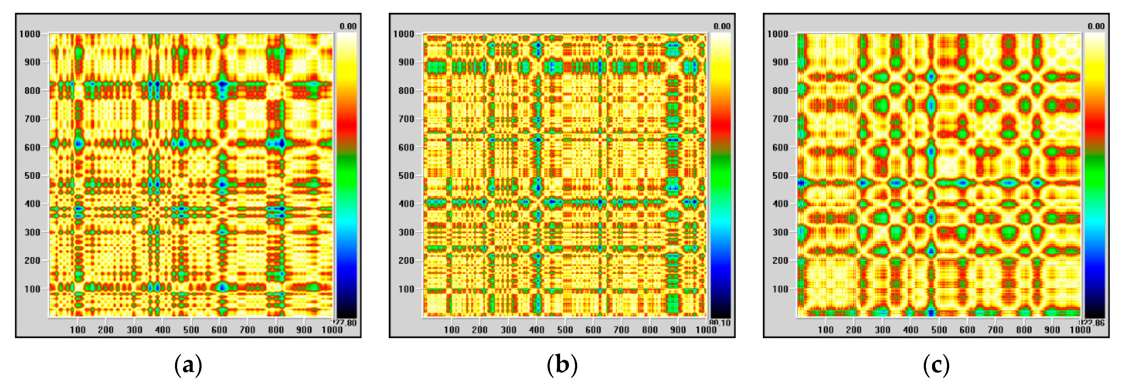
Regarding kurtosis, it has positive average values, but these are lower than 3, except for high values on channels FP1-F7, FP1-F3 and FP2-F4, correlated with the maximum observed for skewness. The behavior of this parameter confirms that, most likely, we are dealing with a focal epileptic seizure. The recurrence map will give us global information about the dynamics of the brain and, for this reason, we will not obtain information about the focal or global characters of the epileptic seizure. The recurrence maps obtained with visual recurrence analysis software for the signal recorded on channel FP1-F7, corresponding to the normal functioning of the brain, the pre-seizure period and the seizure period are represented in Figure 3.

The lack of homogeneity of the maps indicates the existence of a non-stationary signal, and the single points, isolated, indicate strong fluctuations in the system. During the epileptic seizure, the regular component of the system dynamics is much more evident, in agreement with previous observations.

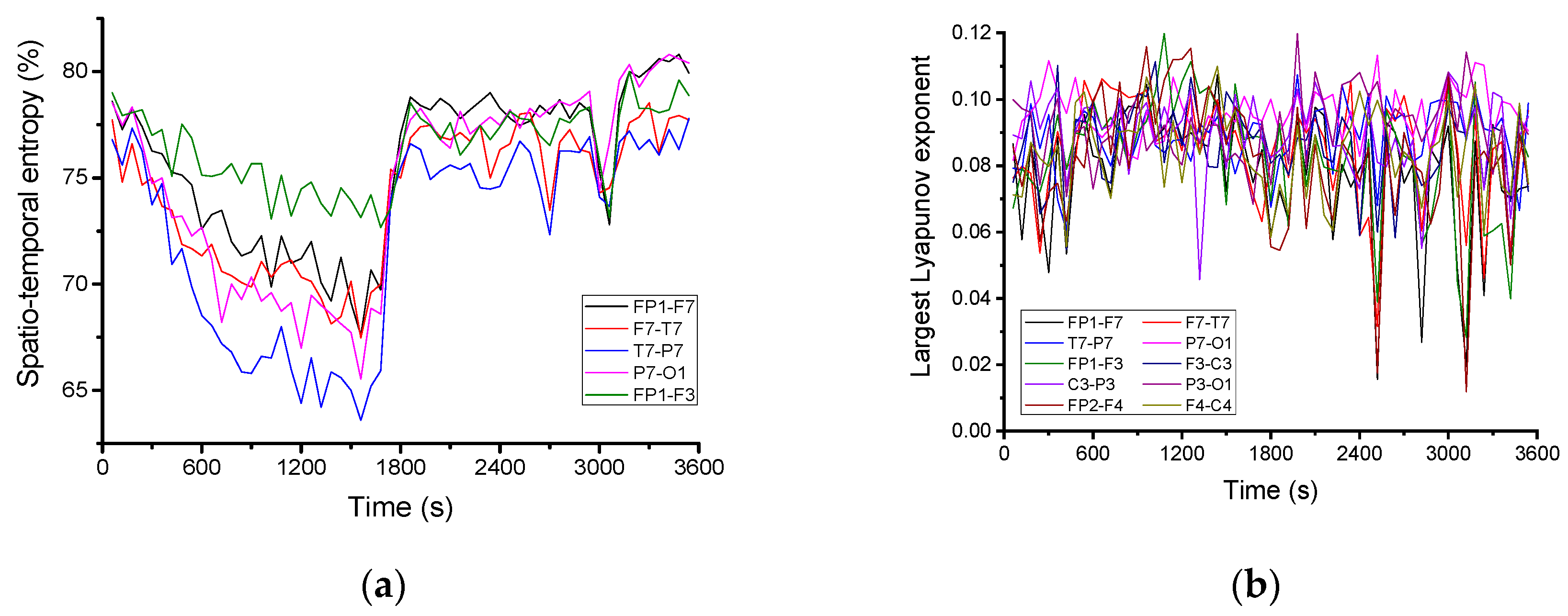
For a more detailed quantitative analysis, the variation in time of the spatio-temporal entropy for 5 channels is represented in Figure 4a. It decreases until the beginning of the pre-seizure period, when it shows rapid growth, remaining at a high value throughout the pre-seizure and seizure periods. On some channels (FP1-F7, FP1-F3 and F7-T7) the existence of several minimums is observed, the spatial–temporal value of entropy decreasing to values close to the regularity limit. In this case, the decrease in the entropy value occurs exactly during the epileptic seizure. Figure 4b shows the time variation of the largest Lyapunov exponent, calculated for 10 channels of the electroencephalogram using the subroutine “Largest Lyapunov exponent” extracted using Santis software. It was found that the largest Lyapunov exponent is positive, with an average value of about 0.09. This means that the brain dynamics are chaotic. During the seizure and the pre-seizure, the largest Lyapunov exponent shows some sharp decreases to values close to zero, i.e., to the regularity limit.

3. The Reconstruction of EEG Signals through Scale Relativity Theory

Common models used to describe neural system dynamics are based on a combination of basic theories derived especially from physics and computer simulations [7,8,9,10]. As such, the description of neural system dynamics implies both computational simulations based on specific algorithms [10,11,12], and developments on usual theories of biophysics, concerning classes of models, developed either on spaces with integer dimensions (differentiable class of models) or on spaces with fractional dimensions and explicitly written through fractional derivatives (non-differentiable class of models) [5,11,12].

A new class of biophysical models can be developed, based on scale relativity theory, either in the monofractal dynamics as in the case of Nottale [13], or in the multifractal dynamics as in the case of the multifractal theory of motion [14]. These models can be used for both simulating and analyzing the EEG signals and can help in their interpretation. To the authors’ knowledge this is the first attempt at representing the information transfer at the neural system level in a multifractal paradigm of motion.

According to the scale relativity theory (Nottale’s model [13] and the multifractal theory of motion [14]), it is supposed that a neural system can be structurally and functionally assimilated to a multifractal object. Then, its dynamics may be described through motions of the neural system’s structural units on continuous and non-differentiable curves (multifractal curves). This means that, in such descriptions, instead of “operating” with a single variable described by a strict non-differentiable function, it is possible to “operate” only with approximations of this mathematical function, obtained by averaging them on different scale resolutions. Consequently, any variable purposed to describe the neural system dynamics will perform as the limit of a family of mathematical functions, this being non-differentiable for null scale resolutions and differentiable otherwise.

Since for a large temporal scale resolution with respect to the inverse of the highest Lyapunov exponent [15,16], the deterministic trajectories of any structural units belonging to the neural system can be replaced by a collection of potential (“virtual”) trajectories, the concept of definite trajectory can be substituted by the one of probability density. It was noted that various applications of this model have been described in [17,18,19,20,21,22,23,24,25,26,27,28,29].

With all the above considerations taken into account, the multifractality expressed through stochasticity, in the description of the neural system dynamics, becomes operational, as we will show in the following.

Therefore, assuming that any neural system can be assimilated to a multifractal object, the dynamics of the neural system’s structural units in the multifractal theory of motion are described through continuous but non-differentiable curves (multifractal curves). According to [14], the following covariant derivative:

$$\frac{\widehat{d}}{dt}={\partial }_t+{\widehat{V}}^l{\partial }_l+D^{lp}{\partial }_l{\partial }_p$$

(1)

where

$$V^l=V_D^l-i{V}_F^l$$

(2)

$$D^{lp}=\frac{1}{4}{\left(dt\right)}^{\frac{2}{f\left(\alpha \right)}-1}\left(d^{lp}+i{\overline{d}}^{lp}\right)$$

(3)

$$d^{lp}={\lambda }_{+}^l{\lambda }_{+}^p-{\lambda }_{-}^l{\lambda }_{-}^p$$

(4)

$${\overline{d}}^{lp}={\lambda }_{+}^l{\lambda }_{+}^p-{\lambda }_{-}^l{\lambda }_{-}^p$$

(5)

$$f\left(\alpha \right)=f\left[\alpha \left(D_F\right)\right]$$

(6)

$$\begin{array}{cc}{\partial }_t=\frac{\partial }{{\partial }_t},{\partial }_l=\frac{\partial }{\partial X^l},{\partial }_l{\partial }_p=\frac{\partial }{\partial X^l}\frac{\partial }{\partial X^p},i=\sqrt{-1},& l,p=1,2,3\end{array}$$

(7)

becomes operational in the writing of motion laws.

In Equations (1)–(7), $t$ is the non-multifractal time with the role of affine parameter of the motion curves, $X^l$ are the multifractal spatial coordinates, $dt$ is the scale resolution, ${\widehat{V}}^l$ is the complex velocity field, $V_D^l$ is the differentiable part of the velocity field independent of scale resolution, $V_F^l$ is the non-differentiable part of the velocity field and is dependent on the scale resolution; ${\lambda }_{\pm }^i$ are constant coefficients associated to differential-non-differential transition, $f\left[\alpha \left(D_F\right)\right]$ is the singularity spectrum of order $\alpha$, $\alpha$ is the singularity index and $D_F$ is the fractal dimension [30] of the “movement curves”.

There are many modes for defining the fractal dimension. Thus, several fractal dimensions may be employed, but the fractal dimension in the sense of Hausdorff–Besikovitch [30] or the fractal dimension in the sense of Kolmogorov are the most commonly used. In the case of many models, selecting one of these definitions and operating it in the context of any neural system dynamics, the value of the fractal dimension must be constant and arbitrary for the entirety of the neural system’s dynamics analysis; for example, it is regularly found that $D_F<2$ for correlative processes in the dynamics of any biological system and $D_F>2$ for non-correlative processes.

In the case where, in the description of neural system dynamics, we operate with $f\left[\alpha \left(D_F\right)\right]$ (i.e., operating simultaneously with several fractal dimensions, on multifractal manifolds, as in the multifractal theory of motion [14]) instead of $D_F$ (i.e., operating with a single fractal dimension, on monofractal manifolds, as in the case of Nottale’s model), a number of advantages can be highlighted: the areas of neural system dynamics that are characterized by a certain fractal dimension, the number of areas in the neural system dynamics, for which the fractal dimensions are situated in an interval of values, and also the classes of universality in the neural system dynamics, even when regular or strange attractors have various aspects.

Now, accepting the scale covariant principle in the description of neural system dynamics, the conservation law of the specific momentum (i.e., geodesic equations on a multifractal manifold) takes the form [14]:

$$\frac{\widehat{d}{\widehat{V}}^i}{dt}={\partial }_t{\widehat{V}}^i+{\widehat{V}}^l{\partial }_i{\widehat{V}}^i+\frac{1}{4}{\left(dt\right)}^{\left[\raisebox{1ex}{$2$}\!\left/ \!\raisebox{-1ex}{$f\left(\alpha \right)$}\right.\right]-1}{D}^{lp}{\partial }_l{\partial }_p{\widehat{V}}^i=0$$

(8)

The explicit form of $D^{lp}$ depends on the type of multifractalization used. It can be admitted that the multifractalization process can take place through various stochastic processes. Amongst the commonly used stochastic processes, the following are mentioned:

(i)

Markovian (thus, memoryless) neural processes. This is the case of scale relativity theory in Nottale’s sense, referring to neural dynamics on monofractal manifolds (with fractal dimension $D_F=2$ [13]);

(ii)

Non-Markovian (thus, exhibiting memory-like qualities) neural processes. Since neural processes usually display some sort of memory-related traits, it is then necessary to operate with mathematical procedures vastly different than the ones mentioned at point (i). This is the case of the multifractal theory of motion, referring to neural dynamics on multifractal manifolds (with various fractal dimensions $D_F$, simultaneously operating) [14].

In this case, wherein it is possible to generalize many of the previous results [17,18,19,20,21,22,23,24,25,26,27,28,29], the following constraints are admitted:

$$\begin{array}{c}\frac{1}{4}{\left(dt\right)}^{\left[\raisebox{1ex}{$2$}\!\left/ \!\raisebox{-1ex}{$f\left(\alpha \right)$}\right.\right]-1}{d}^{lp}=a{\delta }^{lp},\\ \frac{1}{4}{\left(dt\right)}^{\left[\raisebox{1ex}{$2$}\!\left/ \!\raisebox{-1ex}{$f\left(\alpha \right)$}\right.\right]-1}{\overline{d}}^{lp}=b{\delta }^{lp}\end{array}$$

(9)

where $a$ and $b$ are two constant coefficients of multifractal type associated to the differential-nondifferential transition, and ${\delta }^{lp}$ is Kronecker’s pseudotensor. Thus, (8) with the restriction (9) yields:

$${\partial }_t{\widehat{V}}^i+{\widehat{V}}^l{\partial }_i{\widehat{V}}^i+\left(\alpha +i\beta \right){\partial }_l{\partial }^l{\widehat{V}}^i=0$$

(10)

If the complex velocity field (2) is expressed in the form

$${\widehat{V}}^l=-2i\lambda {\partial }^{l}ln\mathsf{\Psi }$$

(11)

with

$$\lambda =\frac{1}{4}\left(a+ib\right){\left(dt\right)}^{\left[\raisebox{1ex}{$2$}\!\left/ \!\raisebox{-1ex}{$f\left(\alpha \right)$}\right.\right]-1}$$

(12)

where $\mathsf{\Psi }$ is the state function of multifractal type, (10) becomes:

$$\left[{\partial }_t-\left(2i\lambda {\partial }^l\ln \mathsf{\Psi }{\partial }_l\right)-i\lambda {\partial }_l{\partial }^l\right]\left(-2i{\partial }^i\ln \mathsf{\Psi }\right)=0, i=\sqrt{-1}$$

(13)

In the usual case [13,14], we could not even write this equation because $\mathsf{\Psi }$ is non-differentiable and therefore its derivatives are formally infinite. However, as we have shown above, the fundamental tool used in scale relativity, which actually aimed to find a solution for such a problem (at the multifractal space–time coordinate level), can now similarly be used at a state function level. Specifically, in terms of a multifractal scale-dependent state function $\mathsf{\Psi }\left(\lambda ,t,dt\right)$, the various terms of (13) remain finite for all values of $dt\ne 0$. We are thus in the same conditions as in the previous calculations involving a differentiable state function, so that it can finally be integrated in terms of a multifractal Schrödinger equation that maintains the same form as the differentiable state function:

$${\lambda }^2{\partial }_l{\partial }^l\mathsf{\Psi }+i\lambda {\partial }_t\mathsf{\Psi }=0$$

(14)

This multifractal-type Schrödinger equation has differentiable solutions that come as a direct consequence of the multifractality of space. Such a result agrees with Berry’s and Hall’s phases, also similar findings obtained in the framework of usual quantum mechanics [31,32,33]. In the particular case of fractalization through a Markov-type stochasticization, i.e., for motions on Peano-type curves at Compton scale resolution:

$$f\left[\lambda \left(D_F\right)\right]\to 2,\lambda =\frac{1}{4}\left(a+ib\right){\left(dt\right)}^{\left[\raisebox{1ex}{$2$}\!\left/ \!\raisebox{-1ex}{$f\left(\alpha \right)$}\right.\right]-1}\left(a\to 0,f\left[\alpha \left(D_F\right)\to 2\right]\right)\to \frac{\hslash }{2m_0}$$

(15)

with $\hslash$ the reduced Planck constant and $m_0$ the system’s structural unit rest mass, (14) is reduced to the standard Schrödinger equation:

$$\frac{{\hslash }^2}{2m_0}{\partial }_l{\partial }^l\mathsf{\Psi }+i\hslash {\partial }_t\mathsf{\Psi }=0$$

(16)

Let us note that, although (16) is fundamental in quantum mechanics, and, through it many neural dynamics can be explained (see [33]), the current context imposes approaching neural dynamics in a much wider framework, namely the one based on the multifractality concept.

Now, let us rewrite (14) for the complex conjugate of $\mathsf{\Psi }$, i.e., $\overline{\mathsf{\Psi }}$, in the form

$${\lambda }^2{\partial }_l{\partial }^l\overline{\mathsf{\Psi }}+i\lambda {\partial }_t\overline{\mathsf{\Psi }}=0$$

(17)

By multiplying (14) with $\overline{\mathsf{\Psi }}$ and (17) with $\mathsf{\Psi }$ and subtracting them we can obtain the multifractal-type state densities conservation law:

$${\partial }_t\rho +{\partial }_l\left(\rho j^l\right)=0$$

(18)

where

$$\mathsf{\Psi }\overline{\mathsf{\Psi }}=\rho ,j^l=i\lambda \left(\mathsf{\Psi }{\partial }_l\overline{\mathsf{\Psi }}-\overline{\mathsf{\Psi }}{\partial }_l\mathsf{\Psi }\right)$$

(19)

In (18) and (19), $\rho$ is the multifractal-type state density and $j$ is the multifractal-type state current density. Therefore, in accordance with the above obtained results, the probability density can become a fundamental concept in the neural dynamics analysis, substituting thus the concept of definite trajectory.

In the following let us first observe that the multifractal-type Schrödinger equation, which is a motion equation for the multifractal-type state function $\mathsf{\Psi }$, is invariant with respect to the multifractal-type Galilei group, in its vectorial form. Then let us observe that the same equation is also invariant with respect to the time and spatial coordinate transformations, which represent a group in itself (different than the multifractal-type Galilei group). These last transformations are, in the most general case of one-dimensional neural dynamics, a result of the multifractal-type SL(2R) group structure, but in two variables with three parameters, through the multifractal-type action [31,32]:

$$\begin{array}{cc}{t}^{\prime }\to \frac{\alpha t+\beta }{\gamma t+\delta },& X^{\prime }\to \frac{X}{\gamma t+\delta }\end{array}$$

(20)

where $\alpha$, $\beta$, $\gamma$ and $\delta$ are real elements.

In accordance with the general mathematical procedures from [31,32], the neural dynamics may be described through a 2 × 2 matrix, with real elements. In a neural system, it is obvious that the problem revolves around a family of such matrices, each of them describing the dynamics of a neural system entity (structural unit). Therefore, the interactions between the neural system entities can be expressed through relations between the representative matrices. These relations must contain certain parameters that characterize the structure of the neural system, adequate to the description of the neural system dynamics.

It results that the matrix that generates the anharmonic curve [31,32] is a 2 × 2 matrix with real elements and can be written as:

$$M=\left(\begin{array}{cc}\alpha & \beta \\ \gamma & \delta \end{array}\right)$$

(21)

Let us observe that the elements of this matrix contain, in an unspecified form, both the physical parameters of the neural system implying neural dynamics and the possible initial conditions of the neural dynamics. Precisely, the elements of matrix (21) depend on the scale resolution in the sense given by the multifractal theory of motion (the neural curves are continuous and non-differentiable, i.e., multifractal curves). In this context, the obtained results will also be in a sense of the previously mentioned theory.

A set of such matrices, with variable elements, may be admitted as relevant for the neural dynamics, for example by means of a fundamental spinor set, given by 2 × 2 matrices that describe the neural dynamics. This description is analogous to the spinor description of spacetime (for details see [34]).

In this situation, any 2 × 2 matrix of form (21) can be written as a linear combination with real coefficients, implying two special matrices, i.e., the unity matrix $U$ and a null-trace matrix $I$ (from involution), which means that:

$$M=\lambda U+\mu I$$

(22)

The involution $U$ has some important properties: its squared form is a multiple of $U$ and also the fixed points of its homographic action are the ones of matrix $M$.

In Equation (22) we could freely choose a parameterization in which the squared form of $U$ can be the unity matrix, up to a sign. In this case the elements of $I$ may be expressed with the help of only two parameters, which represent the asymptotic directions of matrix $M$. If the asymptotic directions are complex, being of the form $u\pm iv$, the representation of the matrix $I$ through asymptotic directions is of a spherical type. Then, satisfying the above-mentioned properties implies, for the matrix $I,$ the form:

$$\begin{array}{cc}I=\frac{1}{v}\left(\begin{array}{cc}-u& -u^2-v^2\\ 1& u\end{array}\right),& I=-U\end{array}$$

(23)

This kind of representation for neural dynamics has an important advantage. When focusing on the physics of the issue, the model allows for an explicit differential description of the neural dynamics, through matrix geometry, identical to the metric geometry of space at a certain moment, the hyperbolic geometry of the second type [35].

The representation of neural dynamics through 2 × 2 matrices then leads us to a natural matrix of the matrices’ space, for example the Killing–Cartan metric of $SL\left(2R\right)$-type algebra of these matrices [36]. The basic co-vectors of such geometry are, in the general case of matrix (21), given by external differential forms:

$$\begin{array}{c}\begin{array}{ccc}{\omega }^1=\frac{\alpha d\beta -\beta d\alpha }{\Delta },& {\omega }^2=\frac{\alpha d\gamma -\gamma d\alpha }{\Delta },& {\omega }^3=\frac{\beta d\gamma -\gamma d\beta }{\Delta }\end{array}\\ \mathsf{\Delta }=\alpha \gamma -{\beta }^2\end{array}$$

(24)

In the parameterization given through (22) and (23), (24) becomes:

$$\begin{array}{c}{\omega }^1=\frac{1}{v}d\Phi +{sin}^2\Phi \frac{du}{v^2}-sin\Phi cos\Phi \frac{dv}{v^2}\\ {\omega }^2=2\frac{u}{v}d\Phi +2{sin}^2\Phi \frac{udu+vdv}{v^2}+2sin\Phi cos\Phi \frac{vdu-udv}{v^2}\\ {\omega }^3=\frac{u^2+v^2}{v}d\Phi +{sin}^2\Phi \frac{\left(u^2-v^2\right)du+2uvdv}{v^2}+sin\Phi cos\Phi \frac{2uvdu-\left(u^2-v^2\right)dv}{v^2}\end{array}$$

(25)

where:

$$tan\Phi =\frac{\mu }{\lambda }$$

(26)

Related to these co-vectors, the metric is given by the squared form:

$$d{s}^2={\omega }^1{\omega }^3-{\left(\frac{{\omega }^2}{2}\right)}^2=d{\Phi }^2-{sin}^2\Phi \frac{d{u}^2+d{v}^2}{v^2}$$

(27)

Therefore, for as long as the neural system is defined by the core property admitted by physics to be essential, i.e., the neural dynamics, its description mode is a metric geometry. In such conjecture, the metric is given through (27), where $\mathsf{\Phi }$ is an arbitrary “phase”, and $u$ and $v$ are “coordinates” obtained from the (local) dynamics of the neural system, in the previously described method.

This kind of approach for neural dynamics can certainly be delegated to harmonic maps, from the neural system to the space. As soon as the mapping mode of the neural system on the available space is solved, the quantities $\mathsf{\Phi }$, $u$, $v$ and the elements of the matrix family that represent the neural system are obtained. In principle, a “position” function will be sufficient to correctly define a specific quantity of the neural system.

The difficulty of representing the neural system in this form can be overcome though the harmonic map $\mathit{X}=\left(X_1,X_2,X_3\right)\to \mathit{\xi }=\left({\xi }^1,{\xi }^2,{\xi }^3\right)$ which can provide a set of quantities as functions of spatial coordinates. Let us now consider the functional corresponding to the harmonic mapping principle (for details see [37]):

$$J=\frac{1}{2}{{\displaystyle \int \int \int }}^{}{d}^3\mathit{X}\sqrt{\left|h\right|}{h}^{il}\left(\mathit{X}\right)\frac{\partial {\xi }^{\mu }\partial {\xi }^{\nu }}{\partial X^i\partial X^l}{g}_{\mu \nu }\left(\mathit{\xi }\right)$$

(28)

where $h$ is the space metric and $g$ is the associated metric of the neural system. Cancelling the first degree variation of this functional, in relation to the spatial coordinates, gives us the harmonic map. Taking into account the fact that the space is Euclidean and using (26) for the metric tensor associated to the neural system, the integrand of (28) can be written as:

$$\sqrt{\left|h\right|}{h}^{il}\left(\mathit{X}\right)\frac{\partial {\xi }^{\mu }\partial {\xi }^{\nu }}{\partial X^i\partial X^l}{g}_{\mu \nu }\left(\mathit{\xi }\right)\equiv {\partial }_l\Phi {\partial }^l\Phi -{\left(\frac{sin\Phi }{v}\right)}^2\left[{\partial }_{l}u{\partial }^{l}u+{\partial }_l\nu {\partial }^l\nu \right]$$

(29)

where the usual notation ${\partial }_l$ denotes the gradient.

Relation (29) can also be written in the form:

$$\sqrt{h}{h}^{il}\left(\mathit{X}\right)\frac{\partial {\xi }^{\mu }\partial {\xi }^{\nu }}{\partial X^i\partial X^l}{g}_{\mu \nu }\left(\mathit{\xi }\right)={\partial }_l\Phi {\partial }^l\Phi +\frac{sin{\Phi }^2}{4}\frac{dhd\hslash }{{\left(h-\hslash \right)}^2}$$

(30)

where

$$h=u+iv,\hslash =u-iv$$

(31)

Now, the phase coherence of neural dynamics, given by restrictions (which corresponds with the beginnings and evolutions of the eclamptic/epileptic seizures)

$$\Phi =\mathrm{const},\Phi \ne 2n\pi ,n=1,2\dots$$

(32)

transforms (30) so that

$$\sqrt{h}{h}^{il}\left(\mathit{X}\right)\frac{\partial {\xi }^{\mu }\partial {\xi }^{\nu }}{\partial X^i\partial X^l}{g}_{\mu \nu }\left(\mathit{\xi }\right)~\mathrm{const}\frac{dhd\hslash }{{\left(h-\hslash \right)}^2}$$

(33)

The restriction (32) can be correlated with scale transitions.

This last expression represents a harmonic map from the Euclidian space to the hyperbolic (Lobacevski) plane, in the Beltrami–Poincaré representation. The Euler equations corresponding to the functional (32) are

$$\left(h-\hslash \right){\partial }_l{\partial }^{l}h=2{\partial }_{l}h{\partial }^{l}h$$

(34)

and its complex conjugate. It can be observed that

$$h=i\frac{coshx+e^{-i\omega }sinhx}{oshx-e^{-i\omega }sinhx}$$

(35)

verifies (33), where $x$ is a solution of the Laplace equation in phase space and $\omega$ is arbitrary (in the sense that it does not depend on the position in space).

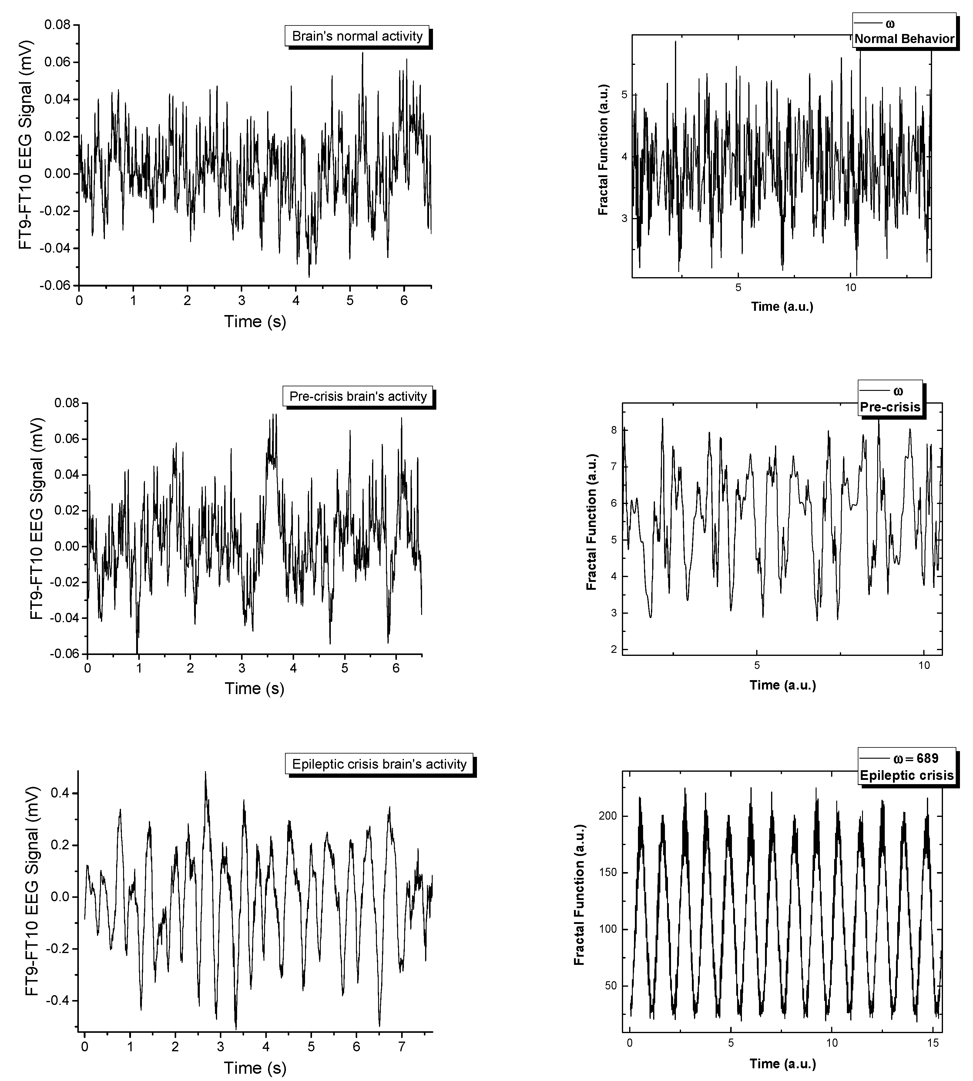
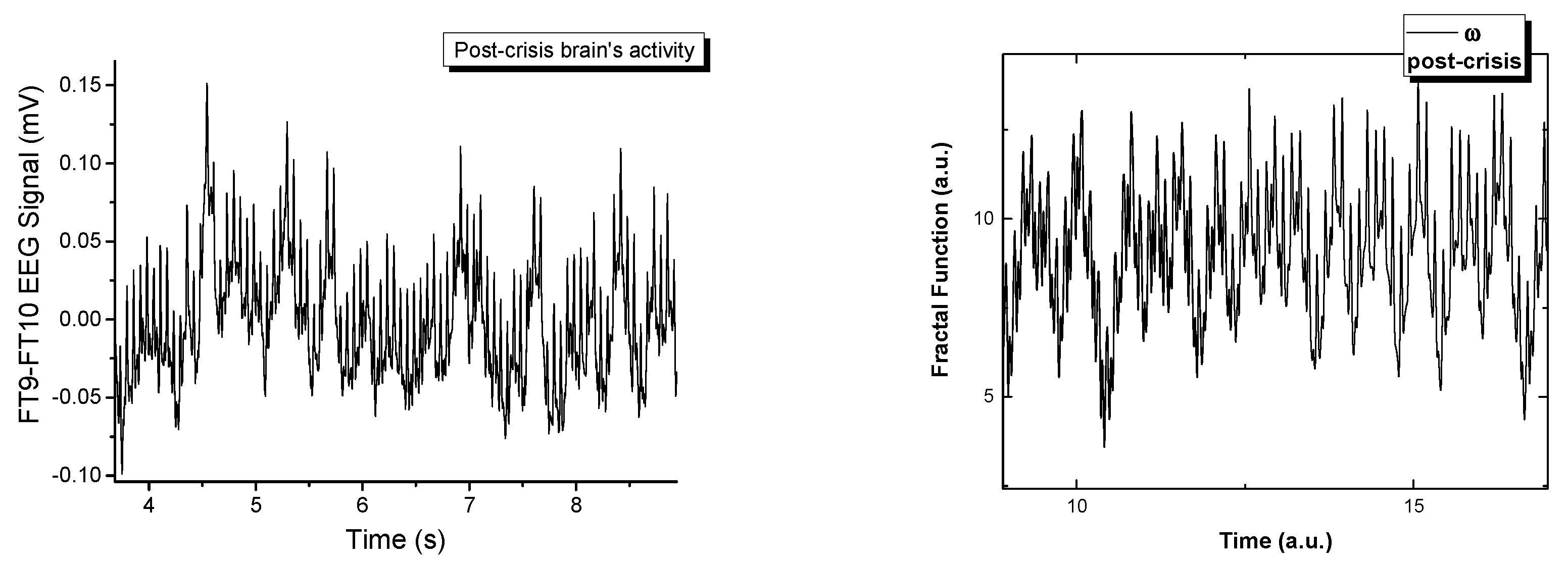
In Figure 5 the real signals and the simulated ones are represented in a comparative manner. The fractal model is a good fit when attempting to recreate signals that are naturally chaotic. There have been extensive publications on the dynamics of the model [38,39,40,41,42,43,44,45,46,47] and it has been shown that the system with single fractality degrees evolves from simple oscillatory behavior to a quasi-chaotic state. This means that a single stream cannot reach chaos. However, the real signal measured from EEG contains a bundle of streams with different properties (amplitude, frequency, fractality degree), therefore we need to apply the same approach when reconstructing the EEG signals in the multifractal paradigm. By using an n-type polynom combination with a randomly selected weight, we reconstructed the signals seen in Figure 5. The multifractal model developed here has a control parameter, ω. By varying the control parameters for the complex multi-stream simulations, we observe a transition similar to the one seen empirically. Each signal is constructed by the polynomic superposition of 6 multifractal strips, each characterized by a different fractal parameter. The normal behavior is a chaotic signal that transitions with the variation of ω towards a sinusoidal-type signal when a fractal resonance is reached between the multifractal streams. This resonating region is unstable and can be found for a small range of values, immediately followed by fractal behavior. From this analysis we can conclude that in the multifractal paradigm the epileptic seizure is defined by a maximum resonance-type state when all the streams move synchronously. This is not an equilibrium state but it is described by clear transition scenarios that can be used to further our understanding of these types of abnormal behavior of the brain.

4. Conclusions

Two complementary operational procedures have been proposed for evaluating and predicting the onset of epileptic and eclamptic seizures. The first procedure analyzes the electrical activity of the brain (EEG signals) using nonlinear dynamic methods, while the second reconstructs any type of EEG signal based on scale relativity theory. Using the non-linear dynamics method, the analysis performed on the signals corresponding to the electroencephalogram of an epileptic patient showed that some statistical parameters, such as standard deviation or variance, as well as the spatial–temporal entropy, can be used to predict in advance the onset of the epileptic seizure. To do this, these parameters (or at least one of them) need to be monitored permanently, and the warning system must be coupled to a system of automatic intervention on the patient, by drugs or electrophysiology, so that the onset of the seizure is prevented. Thus, the basis of a functional electronic device, which can be carried and controlled permanently by the epileptic patient, can be laid (as soon as a sensor notices the occurrence of a dynamic behavior of a pre-seizure type, a treatment that avoids the onset of the epileptic seizure can be administered).

Using methods of scale relativity theory (for example: the time homographic invariance of a Schrödinger equation of a multifractal type, harmonic mappings from the usual space to the hyperbolic one, etc.) various types of EEG signals have been reconstructed. In such context, the explicit differential descriptions of the brain activity in the form of 2 × 2 matrices with real elements were disclosed through the in-phase coherences at various scale resolutions, especially the complex brain neuronal dynamics and sequences of epileptic and eclamptic seizures. In such context, the phase coherence at various scale resolutions has been assimilated to scale transitions established by different fractal degrees of the motion curves (movement curves associated with the dynamics of the neural system’s structural units).