Detecting Anonymous Target and Predicting Target Trajectories in Wireless Sensor Networks

Abstract

Target Tracking (TT) is an application of Wireless Sensor Networks (WSNs) which necessitates constant assessment of the location of a target. Any change in position of a target and the distance from each intermediate sensor node to the target is passed on to base station and these factors play a crucial role in further processing. The drawback of WSN is that it is prone to numerous constraints like low power, faulty sensors, environmental noises, etc. The target should be detected first and its path should be tracked continuously as it moves around the sensing region. This problem of detecting and tracking a target should be conducted with maximum accuracy and minimum energy consumption in each sensor node. In this paper, we propose a Target Detection and Target Tracking (TDTT) model for continuously tracking the target. This model uses prelocalization-based Kalman Filter (KF) for target detection and clique-based estimation for tracking the target trajectories. We evaluated our model by calculating the probability of detecting a target based on distance, then estimating the trajectory. We analyzed the maximum error in position estimation based on density and sensing radius of the sensors. The results were found to be encouraging. The proposed KF-based target detection and clique-based target tracking reduce overall expenditure of energy, thereby increasing network lifetime. This approach is also compared with Dynamic Object Tracking (DOT) and face-based tracking approach. The experimental results prove that employing TDTT improves energy efficiency and extends the lifetime of the network, without compromising the accuracy of tracking.

1. Introduction

TT is a primary and most demanding application of sensor networks that aims to develop models to determine crucial information about the mobility factors, such as the location, velocity, and track of a target [1]. In WSNs, the targets in target tracking algorithms may be in active or passive modes. In active mode, the target is active and forms a part of the employed model, whereas in passive mode the target has no active part in the tracking functionality. This research work concentrates on active target tracking.

The main objective of target tracking is to locate a target and monitor the movement of that target continuously as shown in Figure 1. This may be done with the help of sensors deployed in the sensing environment. The sensors may be placed in the environment, randomly or uniformly, depending on the requirement of the application. This target tracking concept is used in myriad of applications such as agriculture, security, smart homes, and so on. WSN consists of a number of sensor nodes placed in the monitoring area. The sensor nodes are small with low-power sensing unit. There is also a low-cost, low-capacity battery to make the components work. In target tracking, the targets may be positioned statically or may be mobile. The assumption that the position of a target is known apriori [2] drives the algorithms in TT to estimate localized position and path of target using several measurements of target’s transmissions. The metrics that are gaining importance in this application of WSN are Angle of Arrival (AOA), Received Signal Strength Indication (RSSI) [3], Time-Of-Arrival (TOA) and Time Difference of Arrival (TDOA). The techniques that are RSSI-based have been broadly researched and have gained popularity in recent years as they are widely available in wireless devices and extra sensors are not needed. Target tracking algorithm is divided into target detection, localization, and trajectory estimation [4].Active target tracking algorithms give more importance to localization and estimation of paths of a target [5].To deal with the localization problem, various features, viz. TOA, Direction of Arrival (DOA), and RSSI are suggested. Authors of [6,7] exploit the features of RSSI to track targets.

The propagation path-loss model is normally used to perform localization of the target, which in turn enables target tracking algorithms to deduce the position of the target. The assumptions made in the path-loss model are that the channel is an ideal free-space medium, or channel measurements are done extensively. Nevertheless, environmental factors, such as attenuation, multipath propagation, and Non-Line-Of-Sight (NLOS) add more complexity to the challenges of TT algorithms [8]. Owing to all these external factors, TT based on RSSI is infeasible in various applications, and requires a thorough list of measurements of channel [9]. Extensive research has been carried out by researchers around the world, focusing on all the external factors in path-loss models. However, the demerit of these approaches is that the models performed reasonably well only in very limited practical scenarios [10]. If these demerits are mitigated, then WSNs can be effectively used for localization and TT.

Apart from WSN, Global Positioning System (GPS) and Bluetooth can be used as required in various applications [11,12,13]. However, they are not considered to be an optimal solution due to incurred cost in installing additional receivers to track the targets, interferences, and limited coverage.

This paper focuses on reducing the level of energy consumption and increasing the accuracy of tracking using combined KF and clique-based approach. This TDTT model is fed with RSSI values as input and output in the relevant location of the target. As the target moves along a trajectory, clique-based approach for target tracking senses the direction and acceleration of the target and reports the new location of the target in a continuous manner.

The main contributions of this paper include the following:

(1) TDTT model that uses prelocalization-based KF for target detection and a clique-based TT methodology; (2) performance evaluation of TDTT via simulations; (3) comparison of TDTT to DOT and FaceTrack; (4) comparison of TDTT to KF, EKF, DOT, and FaceTrack in terms of accuracy.

In this paper, Section 2 explains related work, Section 3 describes WSN model used in our proposed system, Section 4 elaborates our proposed architecture and results of our approach are presented in Section 5.

2. Related Work

A framework to deal with locating people, finding out their positions, counting people, and tracking their movements was described by Patwari et al. [14]. They also exploited the property of penetrating buildings using radio waves for surveillance [15]. Touvat et al. proposed an RSSI-based trilateration approach to compare ISM868 and Zigbee technique and used path-loss model to map RSSI to distance [16]. However, this did not produce desirable results when used for localization. Bosisio suggested different frequencies for calculating RSSI values for the same distance. These RSSI values were then used to increase the accuracy of the determined distance [17]. This accurate measurement of distance is a crucial factor to achieve an ideal localization and to track the targets more accurately. In [18], various TT techniques based on structure of network were discussed at length.

Accuracy is increased by comparing different RSSI values, as enhanced RSSI accuracy leads to increased accuracy in localization and trajectory estimation [19]. Ceylan et al. suggested different frequencies for measuring RSSI [20]. The same distance was used along with different frequencies to measure different RSSI value. A location detection method employing learning methods was explained by Hanen Ahmadi et al. [21]. They employed a group of regression trees to accurately track the location of a target. The regression trees were formed by capturing the association between RSSI and location of anchor node. RSSI-based localization and techniques to improve accuracy were discussed in detail by S.R. Jondhale [22].

Din et al. [23] presented a clustering-based mating method for direct as well as multihop routing to increase the network lifetime in WSN. Sthapit, P et al. [24] suggested using support vector machine and logistic regression to compute the position. Then maximum and minimum error in position estimation were calculated and tabulated. The average error was found to be 50 cm. Banihashemian suggested a range-free localization technique using neural networks and included the concept of Particle Swarm Optimization (PSO) algorithm for optimization [25].

Conventionally, KF [26] is used for tracking a random target. However, KF is constrained to linear and Gaussian assumptions. Thus, linear measurement model is assumed if KF is to be used for tracking in WSNs. However, real-time target motion is nonlinear, so derivatives of KF like Extended Kalman Filter (EKF) and Unscented Kalman Filter (UKF) are used [27]. In all derivatives of KF, after the nonlinear state is made linear, KF is applied. It is always encouraged to use KF for assessing performance in comparisons.

Fayazi et al. combined Generalized Extended Kalman Filter and Genetic Algorithm II, resulting in reduced energy usage and precise position accuracy [28]. In 2019, S.R. Jondhale proposed a framework using two algorithms, Generalized Regression Neural Network (GRNN) KF and GRNN + UKF, to estimate the location of a target in motion [29].The above method is implemented in isotropic and anisotropic networks and the results showed that it resulted in low localization error rate. A localization scheme based on neural network is portrayed by Po-Jen Chuang that used online training and correlated data to calculate internode distance [30]. This scheme increased localization success rate and in turn resulted in low error rate.

A location fingerprinting database composed of Wi-Fi, RSSI, and geomagnetic field intensity calculated with many devices at a multistory building is presented in [31]. Localization and trajectory inference with Convolutional Neural Network (CNN) and Long Short-Term Memory (LSTM) network was carried out on this database.

It is possible to locate a target using solitary node but this approach results in depletion of energy and enforces more computation load on that particular node. Multiple sensors serve to reduce load on a particular node and hence, energy depletion will be much lower as the nodes cooperate with each other in tracking the target. This collaboration among multiple sensors is mandatory to increase accuracy factor and to decrease energy usage [32].

DOT [33] approach is used to track mobile targets accurately and convey the location of target to mobile user. This approach does not need frequent queries regarding target location as it uses spatial information stored by neighboring nodes to track a moving target and thus reduces energy consumption. FaceTrack [34] is a target tracking framework which is used to construct faces, using the nodes of a spatial region surrounding a target. A target tracking algorithm based on clique, for binary proximity sensor networks, is presented by Javed et al. [35]. This work formed cliques consisting of sensors and achieved less location error in TT.

By analyzing the outcome of all the above related work, it is evident that the following factors affect the accuracy of target tracking functionality in WSN: faulty sensor nodes losing targets, delays in TT, usage of energy, connectivity, aggregation, and so on. A sensor node may become faulty due to common scenarios, namely, depletion of battery, environmental disasters, and failure of hardware. The factor that affects the performance of TT functionality is missing the targets. Targets may be missed due to barriers in the path of target or due to errors made in prediction of trajectory of the target. All efforts made to track targets should be concentrated on minimizing the probability of losing the targets. The next factor in TT is minimizing the delay incurred while tracking the object. The tradeoff between delay and accuracy of tracking algorithm should not be compromised. The essential feature is that the delay is to be reduced while the accuracy of target tracking should be maintained considerably. Another consideration in tracking is the execution time of the algorithm. If the algorithm takes longer than expected duration, then the target would have relocated to some other position. Coverage refers to number of sensors that are deployed in the sensing area. Coverage directly affects the performance of WSN. When coverage is more, accuracy is considerably improved. This limiting factor necessitates energy efficient, adaptive target detection and tracking methodology.

We propose a system that uses KF-based target detection and clique-based target tracking to address the problem of coverage, accuracy, and energy efficiency.

3. WSN Model for Anonymous Target Tracking

In this section, we describe the representation of the entire wireless sensor network, representation of sensors in various modes, energy levels, and target trajectories.

3.1. Rudimentary WSN Representation

A wireless sensor network with ‘M’ nodes is put into operation, for ‘T’ duration, in the designated sensing area. A target is assumed to be in motion in the sensing area. An assumption made in this scenario is that sensors deployed in the area belong to the kind of binary sensors that have a prefixed range for sensing. The sensing range of this kind of binary sensor is denoted as ‘R’. The implication of binary sensor is that it returns ‘1’ if the object to be tracked is present in the sensing range and returns ‘0’ if the object is out of range of the sensing node. This basic model allows computation of the target’s location by obtaining the centroids of reported positions of all sensors within the sensing area at any instant ‘t’. Consider ‘m’ sensors are deployed in ‘Y_t’ locations. Y_t = (x_j, y_j), where j = 1...m. These ‘m’ sensors are responsible for detecting the target within the sensing range R. The future position is estimated using Equation (1).

$$Y_c\left(t\right)=\left(x_c\left(t\right), y_c \left(t\right)\right)$$

(1)

where $x_c\left(t\right)=\frac{{\sum }^m{x}_j}{m}$; $y_c\left(t\right)=\frac{{\sum }^m{y}_j}{m}$.

3.2. Sensor Representation for Detecting Targets

The basic model works perfectly only if target ‘t’ is within the sensing range ‘R’ of a sensor as depicted in Figure 2. This assumption does not hold well in real-life scenarios. The target may not always be in detection range of sensors. It is necessary to revise the basic model to include probability of detection of target by a sensor. The mathematical model of this idea is given in Equation (2).

$$p_{s_i}\left(x,y\right)=\{\begin{array}{c}\alpha , if\left(x,y\right)ϵR_j\\ 0, otherwise\end{array}$$

(2)

where $0 \le \alpha \le 1$;$\left(x,y\right)$ is the position of the target and $R_j$ denotes the detection range of sensor $s_i$. The trajectory of target within the detection range of $s_i$ is modeled as a state covariance matrix P(r|r) which is expressed in Equation (3) and the target location at any time instant r is denoted as ‘l’ and estimated using Equation (4). The sensor $s_i$ detects the target with probability $p_r\left(s_i\right)$ as given in Equation (5).

$$P\left(r|r\right)=\left[{\sigma }_{ij}\right] ;i\ge 1, j\le 4$$

(3)

$$l\left(∆t_r\right)=\left[\begin{array}{c}\widehat{x}\left(r+1|r\right)\\ \widehat{y}\left(r+1|r\right)\end{array}\right]=\left[\begin{array}{c}\widehat{x}\left(r|r\right)+∆t_r.\widehat{x_v}\left(r|r\right)\\ \widehat{y}\left(r|r\right)+∆t_r.\widehat{y_v}\left(r|r\right)\end{array}\right]$$

(4)

$$p_r\left(s_i\right)={\displaystyle \iint }{p}_{s_i}\left(x,y\right).p\left(x,y\right)dxdy$$

(5)

where p(x,y) is the probability density function of the target whose position is $X_p={\left[x,y\right]}^T$ and is computed using Equation (6).

$$P\left(x,y\right)=\frac{1}{2 \pi {\left|\sum \left(∆t_r\right)\right|}^{\raisebox{1ex}{$1$}\!\left/ \!\raisebox{-1ex}{$2$}\right.}}x exp\left(\frac{1}{2}{\left(X_p-l\left(∆t_r\right)\right)}^T{\displaystyle \sum }{\left(∆t_r\right)}^{-1}\left(X_p-l\left(∆t_r\right)\right)\right)$$

(6)

Consider ‘M’ sensors $s_{i1},s_{i2}\dots . s_{im}$ in a WSN covering a target region Y = (x,y), probability of target detection by the sensors present in the network is given by Equation (7).

$$p_{si1 .. }{s}_{i2}\dots . s_{im}\left(x,y\right)=1-{\displaystyle \prod }_{i=i_1}^{i_m}\left(1-p_{s_i}\left(x,y\right)\right)$$

(7)

The joint estimated probability of these ‘M’ tracking sensors is given by Equation (8).

$$p_r\left(s_{i1 ,}{s}_{i2}\dots . s_{im}\right)={\displaystyle \iint }{p}_{s_{i1 ,}{s}_{i2}\dots . s_{im}}\left(x,y\right).p\left(x,y\right)dxdy$$

(8)

3.3. Strategies in Target Tracking

The general strategies in TT are naive activation, random activation, selective activation, and periodic activation. The sensor nodes that are deployed in a sensing region for tracking targets work in three modes viz., communication mode, sensing mode, and data processing mode. Figure 3 displays the various operating modes of a sensor.

3.3.1. Naive Activation

The sensors that are deployed to sense an event or track an object are always in sensing mode in this strategy. This strategy performs poorly in terms of conserving energy, which is a crucial factor in WSNs. Even though this strategy does not aim to conserve energy, it serves as a basic model for comparing with all other strategies, as it offers good quality of tracking. Equations (9) and (10) model this strategy.

$$m_{s,NA}=M$$

(9)

$$P_{t.NA}=M{S}^{\alpha }$$

(10)

3.3.2. Random Activation

A sensor node is alerted to be in tracking mode with probability ‘p’. The merit of this strategy is that not all the sensor nodes are always in sensing mode as in naive activation. Only a portion of sensor nodes deployed in sensing region is activated at any instant ‘t’. To model this strategy, Equations (11) and (12) are used.

$$m_{s,RA}=pM$$

(11)

$$P_{t,NA}=pM{S}^{\alpha }$$

(12)

3.3.3. Selective Activation

At any point in time, only a small fraction of sensors are powered on and are in sensing mode. The remaining nodes are made to be in communication mode. This strategy enables the prediction of the next immediate location of the object under tracking. This information is passed on to neighboring sensors that are in close proximity to the path of target. The nodes that are in communication mode are made to toggle to sensing mode on receiving alerts from other nodes that are in trajectory of the object as shown in Figure 4.

Selective activation is done based on previous history of position of the target. It is assumed that the sensing region is circular with radius ‘r_p’. Let X_b be the original location of the target. X_a = X_s denotes prior location of the target. X_f denotes future location of the target. This strategy uses past history of target’s location to arrive at the future position of the target. In other words, X_f is estimated using X_a. Sensors that are enclosed within a circular area of radius ‘r’ and those that lie around X_f (t + 1) are signaled to toggle to sensing mode. Only sensors that are within sensing range R of the original location X_b (t + 1) are toggled to sense the target. In tracking area, two circular sections may overlap with each other. This causes the sensors that lie within the overlapping area to detect the target. The new future position X_a (t + 1) is estimated by finding out the centroid of locations of all sensors that lie in the overlapping area as shown in Figure 5. The sensors that lie in the covering region with radius ‘r_p’ around the estimated location of target X_f alone need to be switched on and should be in sensing mode at any instant. To model this strategy, Equations (13) and (14) are used.

$$m_{s,SA}=\pi S_p^{2}p$$

(13)

$$P_{t,SA}=\pi S_p^2{S}^{\alpha }$$

(14)

where ‘d’ is the deployment density of sensors.

3.3.4. Periodic Activation

The strategy of periodic activation is as follows: The entire network is switched on and off on a periodical basis. This periodical awakening of the sensors follows standard rhythmic pattern. This can be easily incorporated into any of the other strategies mentioned above and is found to be the most suitable strategy for TT.

Let $T_D$ be cycle period, $t_{ON}$ is active time of the sensors and $m_{s,V}$ is strategy adopted for tracking a target which is expressed in Equations (15) and (16).

$$m_{s,PA}=\frac{m_{s,V{t}_{ON}}}{T_D}$$

(15)

$$P_{t,PA}=\frac{m_{s,V}{S}^{\alpha }{t}_{ON}}{T_D}$$

(16)

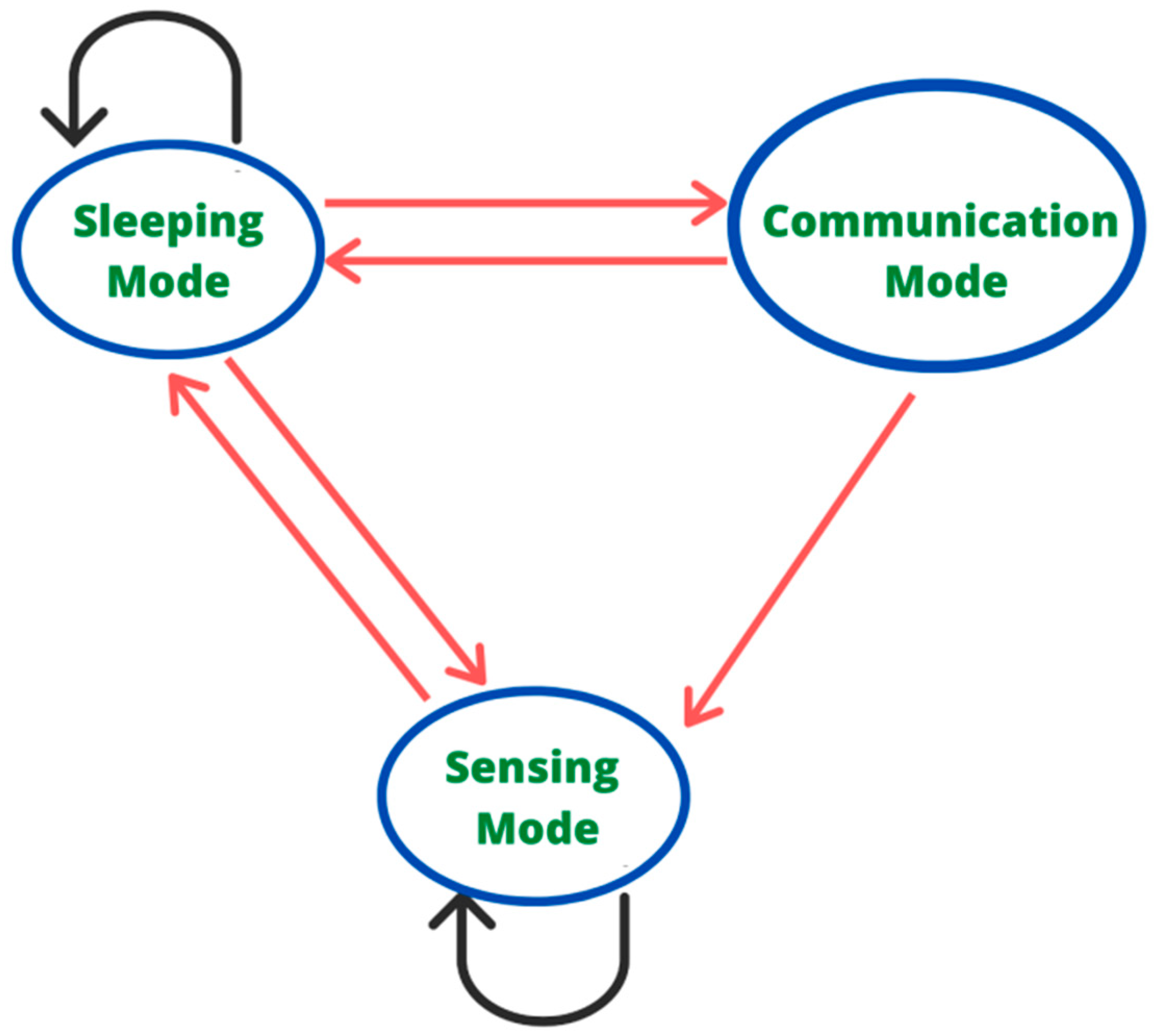
3.4. Representation of Energy in WSN

A sensor node expends energy when it is communicating with other nodes in sensing area, tracking target, and when it is engaged in processing data. A sensor node s_i is considered to be sensing in tracking area and cost of energy that is expended by s_i at each time step is E_rx.

The energy that is expended when a sensor node s_i is communicating with another sensor node s_j is given in Equation (17).

$$E_{t_x}\left(s_i,s_j\right)=\left(e_t+e_d{r}_{ij}^{{\alpha }_c}\right)n$$

(17)

where $e_t$ and $e_d$ are dependent on the transmitter. $r_{ij}$ is the distance between si and sj. α denotes characteristics of the channel. Energy expended for receiving n bits of data is expressed as in Equation (18).

$$E_{r_x}\left(s_j\right)=e_{r{x}^n}$$

(18)

where $e_{rx}$ denotes the specification of the receiver s_j.

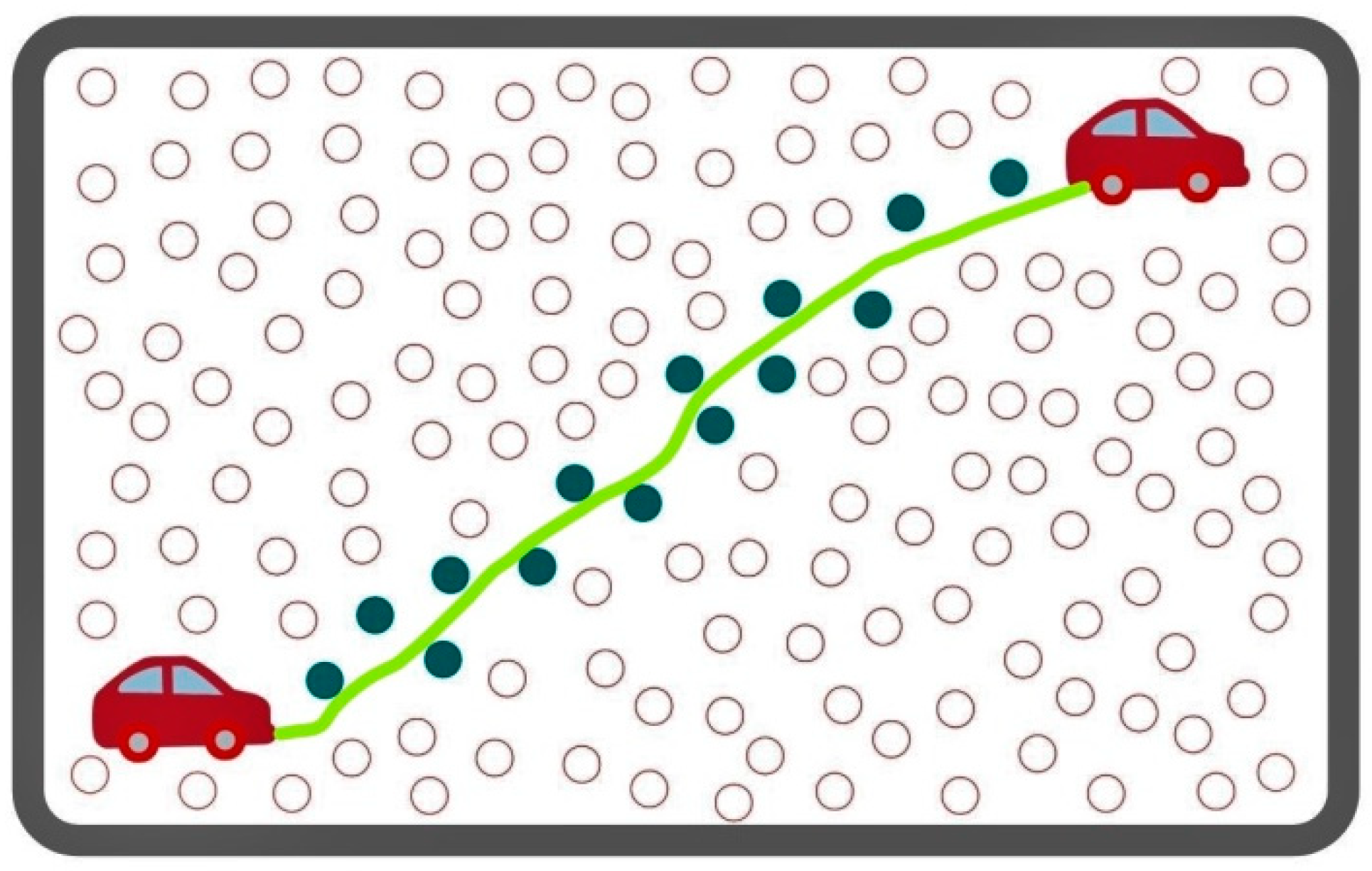
3.5. Representation of Target in Motion

A target in motion is modeled using velocity and location in a 2D sensing region as given in Equation (19).

$$x_m={\left[x\left(m\right)v_x\left(m\right)y\left(m\right)v_y\left(m\right)\right]}^T$$

(19)

where $\left(x\left(m\right),y\left(m\right)\right)$ are the coordinates of the target’s location along x-y plane at time ‘t_m’. ($v_x\left(m\right)v_y\left(m\right))$ are the target velocities along x direction and y direction at time ‘t_m’, respectively. The model that is used to describe target in motion in x-y plane is of stable velocity and is characterized by Equation (20).

$$\begin{gathered} x_{m+1}=F_m{x}_m+G_m{w}_m \\ {F}_m=\left[\begin{array}{c}1 ∆t_m 0 0\\ 0 1 0 0\\ 0 0 1 ∆t_m\\ 0 0 0 1\end{array}\right] \\ {G}_m=\left[\begin{array}{c}\begin{array}{cc}\frac{∆t_m^2}{2}& 0\\ ∆t_m& 0\\ 0& \frac{∆t_m^2}{2}\end{array}\\ \begin{array}{cc}0& ∆t_m\end{array}\end{array}\right] \end{gathered}$$

(20)

The sampling period between two successive recordings t_m+1 and t_m is given by Equation (21).

$$∆t_m=t_{m+1}-t_m$$

(21)

$$w_m={\left[w_x{w}_y\right]}^T$$

(22)

Equation (22) denotes noise sequence whose distribution n is Gaussian. This white Gaussian noise distribution considered here has zero mean and covariance matrix C_w. Therefore, noise across x and y axis is modeled using w_x and w_y. Covariance matrix C_w is given by Equation (23).

$$C_w=\left[\begin{array}{cc}{\sigma }_{w_x}^2& 0\\ 0& {\sigma }_{w_y}^2\end{array}\right]$$

(23)

A few assumptions made in the model are summarized below:

• w_x is not correlated to w_y.
• Covariance and mean of multiplicative noise is given.
• Covariance and mean of additive noise is also given.
• Another crucial assumption is that if noises are absent, then it is fairly straightforward to determine position of the target.

4. Materials and Methods

4.1. Proposed TDTT Model

The architecture of the proposed approach is depicted in Figure 6. The first step in this approach is periodic activation of sensors in sensing area. The activated sensors employ prelocalization and KF to track targets in their surroundings. If target is detected, then sampling interval is varied accordingly and this information is passed onto the cluster head. The next step is to activate sensors based on this sampling interval. This step is followed by identification of successive sensor clusters. These clusters are formed dynamically by constructing cliques.

4.2. Pre-Localization

The first step in target detection is prelocalization which uses maximum likelihood for estimation of target’s position. Consider an example scenario, in which ‘n’ sensors (where n ≥ 3) is in sensing mode and they are tracking targets simultaneously at time ‘t_m’ and noises that are measured by different sensors are exclusive and independent of other sensors defined by N = {N_i}; i = 1,..., n and $P\left(N|(x,y\right)$) denotes conditional probability density function of N. The idea behind using Maximum Likelihood Estimation (MLE) to predict unidentified target locations (x,y) is that if $p(N|\left(x,y\right))$ is maximized, the location of the target can be identified. The mathematical model for the above explained concept is given in Equation (24), assuming measurement noises of sensor are independent and exclusive.

$$P\left(N|x,y\right)={\displaystyle \prod }_{i=1}^{n}P\left(N_i | x,y\right)$$

(24)

Assuming that unknown distance between a target and a sensor, d_i is very small, probability density function can be rewritten as given in Equation (25). The minor approximation done is negligible in probability density function and it is a well-known fact that KF is very resistant towards small variations in measurement noise.

$$P\left(\left\{N_i|x,y\right\}\right) \cong \frac{1}{\sqrt{2\pi }{\sigma }_{N_i}}exp\left\{-\frac{{\left[\left[1+{\mu }_r\right]d_i-\overline{N_i}\right]}^2}{2 {\sigma }_{N_i}^2}\right\}$$

(25)

where $\overline{ N_i}=N_i-{\mu }_n$ and denotes actual calculated measurement. Based on Equation (26), MLE of (x,y) is calculated using Equation (26).

$$\left(\overline{x},\overline{y}\right)={arg}_{min}\left(x,y\right)f\left(x,y\right)$$

(26)

$$f\left(x,y\right)={\displaystyle \sum }_{i=1 }^n\frac{{\left[\left[1+{\mu }_r\right]d_i-\overline{N_i}\right]}^2}{2 {\sigma }_{N_i}^2}$$

(27)

Equation (27) has to be minimized and this is quite difficult as f(x,y) is not linear. Newton-Raphson method, an iterative optimized solution, is used to process this non-linear function. This step works as follows:

Step 1: compute x⁽ⁱ⁺¹⁾ and y⁽ⁱ⁺¹⁾ using Equation (28) where h is step size.

$$\begin{gathered} \left[\begin{array}{c}{x}^{\left(i+1\right)}\\ y^{\left(i+1\right)}\end{array}\right]=\left[\begin{array}{c}{x}^i\\ y^i\end{array}\right]-h{H}^{-1}\left(x^{\left(i\right)},y^{\left(i\right)}\right).\nabla f^T\left(x^{\left(i\right)},y^{\left(i\right)}\right) \\ \nabla f\left(x^{\left(i\right)},y^{\left(i\right)}\right)={\left[\begin{array}{cc}\frac{\partial f\left(x,y\right)}{\partial x}& \frac{\partial f\left(x,y\right)}{\partial y}\end{array}\right]}_{x=x^{\left(i\right)}, y=y^{\left(i\right)}} \\ H\left(x^{\left(i\right)},y^{\left(i\right)}\right)={\left[\begin{array}{cc}\frac{{\partial }^{2}f\left(x,y\right)}{\partial x^2}& \frac{{\partial }^{2}f\left(x,y\right)}{\partial x\partial y}\\ \frac{{\partial }^{2}f\left(x,y\right)}{\partial y\partial x}& \frac{{\partial }^{2}f\left(x,y\right)}{\partial y^2}\end{array}\right]}_{x=x^{\left(i\right)},y=y^{\left(i\right)}} \end{gathered}$$

(28)

Step 2: iterate step 1 until $\left|x^{\left(i+1\right)}-x^{\left(i\right)}\right|<\epsilon$ and $\left|y^{\left(i+1\right)}-y^{\left(i\right)}\right|<\epsilon$ with step size ‘1′ and $\epsilon >0$ is a fixed limit.

The first and third terms of the estimated value ${\widehat{x}}_{m|m-1}$ of KF are ${\widehat{ x}}_{m|m-1}^1$ and ${\widehat{ x}}_{m|m-1}^3$. This iterative method converges and gives a global minimum in successive iterations. The initial values assigned to first and third terms of initial prediction in KF play an important role in making this prediction an accurate one, based on the constraint that the sampling period is limited.

4.3. Position Estimation Using KF

After prelocalization, the result is the changed measurement.

$$\overline{N_m}={\left[\overline{x}\left(m\right) \overline{y}\left(m\right)\right]}^T$$

(29)

Equation (29) has linear representation which is shown in Equation (30).

$$\overline{N_m}=\left[\begin{array}{ccc}1& 0& \begin{array}{cc}0& 0\end{array}\\ 0& 0& \begin{array}{cc}1& 0\end{array}\end{array}\right]x_m+v_m=Z{x}_m+V_m$$

(30)

V_m denotes measurement noise that is converted after prelocalization. This N_m value is to be used in KF. Equation (31) shows Baye’s rule for posterior probability distribution.

$$P((x,y)|N)=\frac{P(N|x,y) P_b\left(x,y\right)}{P\left(N\right)}$$

(31)

The prior probability density function of (x,y) that is known to sensor nodes is p_b(x,y). However, p_b (x,y) does not include any information on the previous position of the target under consideration. p_b (x,y) is uniform, always in sensing region. Considering this, $P\left(x,y|N\right)$ is shown in Equation (32).

$$P\left(x,y|N\right)= \alpha P(\left(N|x,y\right)$$

(32)

$$(x,y) \mathrm{is} \mathrm{independent} \mathrm{of} \alpha . \mathrm{Therefore}, P \left(x,y|N\right)=\frac{\alpha Xexp\left(-f\left(x,y\right)\right)}{{\left(2\pi \right)}^{\raisebox{1ex}{$n$}\!\left/ \!\raisebox{-1ex}{$2$}\right.}{\prod }_{i=1}^n{\sigma }_{N_i}}$$

(33)

The equation after prelocalization and approximation is given in Equation (34).

$$f\left(x,y\right)\cong f\left(\overline{x},\overline{y}\right)+\frac{1}{2}{\left[\begin{array}{c}x-\overline{x}\\ y-\overline{y}\end{array}\right]}^{T}H\left(\overline{x},\overline{y}\right)\left[\begin{array}{c}x-\overline{x}\\ y-\overline{y}\end{array}\right]$$

(34)

$H\left(\overline{x},\overline{y}\right)$ denote Hessian matrix shown by Equation (35).

$$H\left(\overline{x},\overline{y}\right)=\left[\begin{array}{cc}\frac{{\partial }^{2}f\left(x,y\right)}{\partial x^2}& \frac{{\partial }^{2}f\left(x,y\right)}{\partial x\partial y}\\ \frac{{\partial }^{2}f\left(x,y\right)}{\partial y\partial x}& \frac{{\partial }^{2}f\left(x,y\right)}{\partial y^2}\end{array}\right]x=\overline{x} ,y=\overline{y}$$

(35)

$$P \left(x,y|N\right)\cong \beta exp\left(-\frac{1}{2}{\left[\begin{array}{c}x-\overline{x}\\ y-\overline{y}\end{array}\right]}^{T}H\left(\overline{x},\overline{y}\right)\left[\begin{array}{c}x-\overline{x}\\ y-\overline{y}\end{array}\right]\right) \mathrm{where} \beta \mathrm{is} \mathrm{a} \mathrm{constant}$$

(36)

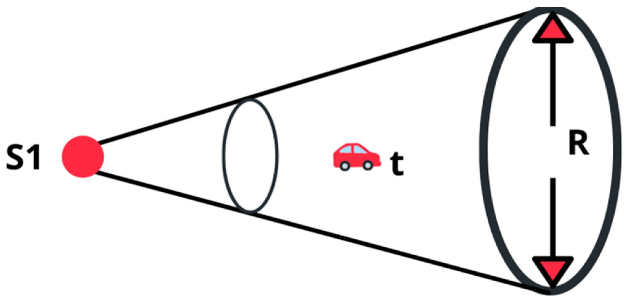
4.4. Choosing Sampling Period

Assuming sampling period $∆t_m$ to be uniform does not make the representation energy efficient and cannot adapt to the trajectory of target. The interval of sampling is denoted by $\left[T_{min}, T_{max}\right]$. This interval is chosen so that $T_{min}$ is greater than the time taken for communication, sensing, and processing, whereas, $T_{max}$ should not be arbitrarily larger values, as the model has to deal with changing trajectory of the object. Considering the difficulty of choosing sampling period and predictions made in covariance matrix, for approximation, a time update is performed to calculate the sampling period.

Uncertainty in estimated position is shown in Equation (37).

$$\begin{gathered} \varnothing \left(m+1 | m\right)=trace\left({\displaystyle \sum }\left(∆t_m\right)\right) \\ =\left({\sigma }_{11}+{\sigma }_{33}\right)+\left(2{\sigma }_{12}+2{\sigma }_{34}\right)∆t_m+\left({\sigma }_{22}+{\sigma }_{44}\right)∆t_m{}^2+\frac{2}{3}q∆t_m{}^3 \\ =\varnothing \left(m | m\right)+\left({\sigma }_{11}+{\sigma }_{33}\right)+\left(2{\sigma }_{12}+2{\sigma }_{34}\right)∆t_m+\left({\sigma }_{22}+{\sigma }_{44}\right)∆t_m{}^2+\frac{2}{3}q∆t_m{}^3 \end{gathered}$$

(37)

If $P \left(m | m\right)>0$ and c(m) > 0 and ${\varnothing }_0>\varnothing \left(\mathrm{m} | \mathrm{m}\right)>0$, then there is the possibility of a real root that is positive. Based on Equation (37), two possible modes of operation in TT are quick tracking and tracking management. When $\varnothing \left(m | m\right)>0$ is not satisfied, then quick tracking is employed, usually when tracking is initiated or when target changes the course. The sampling period is selected as $T_{min}$. When there is an acceptable accuracy in recent and estimated tracking, tracking management mode is employed. The sampling period is greater than $T_{min}$ and the value is the least value among positive root of Equation (37) and $T_{max}$.

4.5. Choosing Sensors to Be in Sensing Mode

After determining sampling period values, sensors will be chosen for sensing. A related assumption is that sensor nodes store the characteristics of all of its neighboring sensor nodes, namely, position and sensing range. The cluster head chosen now evaluates probability density function of other sensors, considering the estimated position of target and associated covariance matrix. The neighboring sensor nodes are denoted as a set S. Probability density function is computed and sensor with high probability density function at the next step is chosen as the first and foremost member of cluster at time m+1.

$$g_1^{\left(m+1\right)}=ar{g}_{S_i}max\left\{P_r\left(S_i\right) : S_i \in S\right\}$$

(38)

where (m + 1) is the (m + 1)th time step.

The second sensor of the cluster is chosen based on

$$g_2^{\left(m+1\right)}=ar{g}_{S_i}max\left\{P_r\left(g_1^{\left(m+1\right)},S_i\right) : S_i \in S\backslash \left\{g_1^{\left(k+1\right)}\right\}\right\}$$

(39)

$P_r\left(g_1^{\left(m+1\right)},S_i\right)$ is joint distribution probability of $g_1^{\left(m+1\right)} \mathrm{and} S_i$.

$S\backslash \left\{g_1^{\left(k+1\right)}\right\}$ is the set of all sensors S exclusive of $g_1^{\left(m+1\right)}$.

This is employed to choose all other sensors. The jth sensor is chosen as,

$$g_j^{\left(m+1\right)}=ar{g}_{S_i}max\left\{P_r\left(g_1^{\left(m+1\right)},g_2^{\left(m+1\right)}, \dots ., g_{i-1}^{\left(m+1\right)},S_i\right) : S_i \in S\backslash \underset{y=1}{\overset{y=i-1}{{\displaystyle \cup }}}\left\{g_y^{\left(k+1\right)}\right\}\right\}$$

(40)

The selection of sensors is ended when joint distribution probability is greater than a specified limit ${\varnothing }_{\mathrm{t}}$. The tasking cluster for the next iteration is given in Equation (41).

$$G\left(m+1\right)=\left\{g_j^{\left(k+1\right)}:j=1,2,\dots , n\right\}$$

(41)

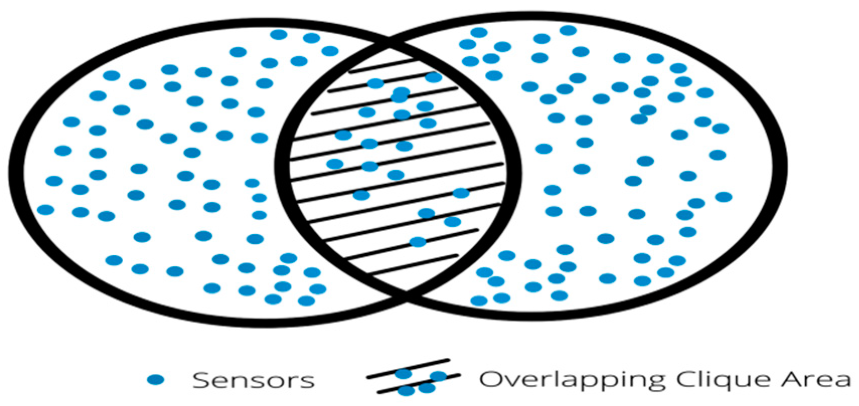
4.6. Identification of Successive Cliques

A target ‘t₁’ is assumed to have unpredictable velocity such that ‘t₁’ is assumed to move in a complex way and it is difficult to represent the complexity. The sequence of steps that is required to identify the clique in which the target ‘t₁’ is travelling is:

• t₁ is detected by s₃.
• s₃ exchanges this information with the neighbors.
• s₃ receives the information from all other neighbors and conducts the comparison between its own information and the neighbors’ information.
• All the neighboring sensor nodes are in sensing mode and t₁ is tracked within the sensing region and the immediate neighbor closest to t₁ maintains the required information.
• The clique in which t₁ moves is constructed.

t₁’s movement from F₁ to any other clique F_j is tracked using monitor and backup operation. This operation is based on all locations of t₁, considering the current motion trajectory. The next step to be carried out is calculating the direction of target’s motion. The clique that is constructed in the previous step is represented by set M_n,

$$M_n=\left\{l_j,{\theta }_m,{\theta }_m^{\prime },v_n^{max},v_n^{ma{x}^{\prime }}\right\};$$

(42)

To calculate the next position of target, it is necessary to calculate $S^{\prime }=S_j;j=1,2,\dots ;$.

The median of this set $S^{\prime }$ is calculated and stored in $S_{median}$. $l_{j+1}$ is calculated and $l_j$ is updated by $l_{j+1}$ and stored. The moving path is calculated based on $l_j;j=1,2,\dots ;$. t₁’s center of gravity position is used to find t₁’s position. t₁ may follow any dynamic path such as travelling in a linear fashion, turning towards right or left, and performing U turn.

In this scenario, time instance of S is subdivided into discrete series, namely S₁, S₂... In each S_i, the duration is set to 1. The direction of movement and target is denoted by $\theta$. The state of motion of target t₁ at time S is denoted by

$$D_{t_1}=\left\{l_j,{\theta }_h,{\theta }_h^{\prime },v_{t_1}^{max},v_{t_1}^{ma{x}^{\prime }}\right\}$$

(43)

${\theta }_h \mathrm{and} {\theta }_h^{\prime }$ are the angle of tracking and the angle of maneuvering.

$v_{t_1}^{max} and v_{t_1}^{ma{x}^{\prime }}$ are the velocity of straight movement and the velocity of maneuvering, respectively.

The distance covered by target t₁ can be calculated by each node in the following ways:

Case 1: Straight Line

$$\begin{gathered} {\theta }_h=0;t \mathrm{is} \mathrm{in} \mathrm{straight} \mathrm{line} \mathrm{motion} \\ {D}_h=v_t^{max} \end{gathered}$$

(44)

Case 2: Curved Line

${\theta }_h\in \left(-\pi ,\pi \right)\&h_1<1$, this denotes $t_1$ is moving in random way (curved). In order to calculate the sequence of locations, it is necessary to introduce $\delta \mathrm{and} r, \delta$ denotes the curve made by the manoeuvring of the target and r denotes the distance covered by t₁ in ${\theta }_h$ direction.

The length of the path due to straight line movement of t₁ is p, then

$$\delta ={\theta }_h^{\prime }P$$

(45)

$$h_1=\frac{\delta }{V_{t}ma{x}^{\prime }}$$

(46)

$${\theta }_h^{\prime }=\frac{V_{t}max}{p}\tan \left({\theta }_h\right)$$

(47)

$$D_h=2p\sin \left(\frac{{\theta }_h^{\prime }}{2}\right)+V_{t}max\left(1-\frac{{\theta }_h^{\prime }p}{V_{t}ma{x}^{\prime }}\right)$$

(48)

Case 3:

$${\theta }_h\in \left(-\pi ,\pi \right)\&h_1\ge 1$$

(49)

$$D_h=2p\sin \left(\frac{V_{t}ma{x}^{\prime }}{2p}\right)$$

(50)

Knowing the current location of t₁ and h, the estimated location of l_j+1 with approximate coordinates $\left(x_{j+1},y_{j+1}\right)$ of t₁ at j + 1 is

$$x_{j+1}=x_j+D_{t_1}\cos {\theta }_h$$

(51)

$$y_{j+1}=y_j-D_{t_1}\sin {\theta }_h$$

(52)

All positions of t₁ can be calculated by changing ${\theta }_h$ between −π and π.

Knowing clique F_j, where t₁ is in motion currently, the sequence of positions is obtained by the previous step. An alert message is issued to the neighbors of F_i. If the node that receives the alert is the requested node, then all those nodes are grouped in F_j+1 and other cliques. If it does not receive the signal, then the node is in awakening state. If t₁ is detected and signal is received, then exchange communication with new backup and proceed with calculating the new maneuver of t₁. Finally, if target t₁ is detected in F_j+1 then l_j is the new location. F_j = F_j+1 is the new clique.

The algorithm for TDTT model is given below (Algorithm 1).

Algorithm 1 TDTT Model

1. Activate sensor at regular interval.

2. Apply prelocalization on the set of activated sensors.

3. Apply Kalman filter.

4. If no target detected then go to step 1.

5. Select neighboring set of sensors.

6. Recalculate sampling period.

7. Exchange information about target with its neighbor.

8. Track target’s clique using monitor and backup operation.

9. Compute direction of target’s motion.

5. Results

In this section, the performance of the proposed approach is evaluated in two different simulation scenarios. The first and second scenario were simulated both in ideal and non-ideal setup to test the performance of tracking the target using KF and clique-based approach. The third scenario was simulated and performance of our approach is compared with DOT and FaceTrack approaches. Both DOT and FaceTrack authors specify an approach that constructs faces to track a target. TDTT constructs cliques similar to Face construction. Therefore, these two approaches are used for comparison. The simulation was performed on a 1000 × 1000 m² field with around 950 sensors in a 40 × 40 grid and a sensing range of 100 m per sensor. The monitored area of this simulation was set to 1000 m and parameters were captured by playing the simulation until 2500 s.

5.1. Scenario 1

In this scenario, it was decided to have field size as constant and vary density ρ and radius of the sensors. Various trajectories were generated using geometric random walks, setting each walk to 10–15 steps. Each step was assumed to be taken in a random direction and continued in the same direction and was made to turn in the other direction. After multiple simulations, it was found that the estimated trajectory is more or less following the original trajectory of the target as shown in Figure 7. In order to estimate the probability of target detection using TDTT, sensing range of sensor was set to 50 m. It was observed that when the distance between target and the sensor under consideration increased, the target detection rate decreased as shown in Figure 8.

This observation led to another experiment in which we varied the density of sensors and the error in localizing the target and tracking the target was calculated. Fixing the size of the field and the radius as constant, the number of sensors in the field was varied from 100 to 650. Then the simulation was performed for uniform regular and random arrangement of sensors. As per spatial resolution theorem, an increase in density of sensors results in a decrease in error estimation. It was noticed that as the number of sensors increased, error in difference between the original and estimated trajectory decreased as shown in Figure 9. There is a slight deviation between theoretical value and estimated error averaged over 55 rounds of random walk paths. The distribution of sensors was kept constant at 950 sensors but their sensing radius was changed from 50 m to 350 m. Error in estimation was found to be decreasing with increase in radius R as shown in Figure 10. The calculated error was more or less in line with the theoretical value.

5.2. Scenario 2

This scenario was simulated by making the following assumptions: sensing range of all the sensors was fixed. The number of sensors was varied from 100 to 650. For each variation of sensor density, the target was deployed either closer to or far off from the sensor arrangement. Initially, the target was deployed closer to the sensor arrangements for all variations in number of sensors and the result was displayed in Figure 9. Then it was decided to vary the position of target deployment for different sensor densities to assess the effect of proximity of sensors on position estimation. Thus, in sensor field with 200 to 400 sensors, the target was deployed closer to the area in which the sensors were concentrated, between 400 to 600 sensors, the sensors were deployed farther away from the target and for the third case, above 600 sensors, we set the target closer to the region where sensors were distributed. It was observed that the simulation yielded predictable results. Even though sensors were populated densely, proximity of sensors close to the target decided the error in position estimation as shown in Figure 11.

In Figure 11, when the sensor density was below 400, the target was deployed closer to the sensor arrangement and there was a decrease in error of estimation. However, when the target was deployed farther away from the concentration of sensors, even when the sensor density was increased to between 400 and 600, there was a noticeable increase in error. Above 600 sensors, the target was closer to the sensor arrangement and subsequently, resulted in reduced error.

5.3. Scenario 3

In scenario 3, the nodes in the network are set to have uniform communication range (c) and sensing range (r) with nil background noise. The communication range is set to greater than or equal to twice the sensing range as given in Equation (53).

$$c\ge 2\ast r$$

(53)

The sensing range of nodes is set to 100 m and communication range of nodes is 200 m. Node–sink synchronization happens in the first 1–10 ms of the simulation. The target’s speed is 1 m/s.

Initially, all sensor nodes collect information regarding neighbor nodes. The target is deployed in the simulated network at an arbitrary time and in a random spot. The target moves in random fashion in the sensing area. Target detection is triggered when the target is detected by the sensor nodes in the network and KF is employed to assess the location of the deployed target. Then the clique is constructed as the target moves along a trajectory. Now the sensors are enabled to track the target. Over 150 simulation runs are carried out and the results are averaged. The initial energy of all nodes is fixed as 50 J. CC2420 radio parameters are used in simulations for communication between the sensor nodes in the network. Three modes of CC2420 radio are transmit, listen, and sleep. The power expended in sleep mode is minimal compared to the other two modes. Based on the clique constructed as the target moves in the sensing region, only those nodes that fall within the clique region are made active and the rest of the nodes that are not in proximity to the target are made to sleep. The comparison of the number of nodes that are asleep during target tracking made by applying DOT, FaceTrack and TDTT approaches is presented in Figure 12.

The proposed TDTT model is compared to FaceTrack and DOT in terms of energy consumed by the nodes as shown in Figure 13. Even though the concept of sleep node is employed in FaceTrack and DOT, the number of sleep nodes in TDTT is comparatively higher than the other two approaches, which results in relatively lower energy consumption, without compromising the accuracy of tracking the target.

In order to calculate the network lifetime, we deployed a target to traverse through the network 1000 times in random fashion and applied DOT, FaceTrack, and TDTT approaches for target tracking. As the simulation progressed, we monitored the nodes that went dead and the summarization of dead nodes is presented in Figure 14.

5.4. Comparison of TDTT with Other Existing Approaches in Terms of Accuracy

In order to assess the tracking performance of TDTT, we deployed a target to traverse through the network 1000 times in random fashion at random velocity range of (0, 30) m/s. Then we applied KF, EKF, DOT, FaceTrack, and TDTT approaches. The observed accuracy for all the approaches is illustrated in Figure 15. The probability of error in tracking increases as the target moves at a faster rate with increasing velocity. Hence, the accuracy of TDTT decreases as the target moves at a faster pace. It was observed that TDTT and FaceTrack achieved more or less the same accuracy. KF performed poorly compared to EKF in this random movement scenario. DOT performed moderately in terms of accuracy.

5.5. Assessment of Energy Consumption and Accuracy

In order to assess energy consumed and accuracy achieved in TDTT, another scenario was simulated with 250 nodes in a 500 × 500 m². The motion of the target was set to linear and around 1000 steps were taken by the target. The velocity was set between 0 m/s and 30 m/s randomly.

Initially, energy consumed by TDTT with respect to increase in velocity was observed. In Figure 16, across the horizontal axis, velocity of target is displayed and average energy consumption is shown across the vertical axis. From the figure, we can see that TDTT activates a lower number of sensors for tracking at low velocities. However, at higher velocities, as expected, TDTT may consume more energy. We can conclude that at lesser velocities, TDTT performs considerably better than at higher velocities.

The next experiment is in regards to accuracy of TDTT at low and high velocities. Any approach would suffer from loss of accuracy at higher velocities. However, from Figure 17, we can conclude that the accuracy in TDTT at higher velocities is still adequate for the majority of applications. The association between energy saving and accuracy in various scenarios may still pose serious apprehensions. We would like to explore this association in greater depths in future work.

6. Conclusions and Future Works

This paper focuses only on clique-based single target tracking scenario, where the clique is formed dynamically along the path of the target in motion. At the end of each time step, the sensor nodes around the moving target become activated and the rest of the sensor nodes will be deactivated. This results in reducing energy consumption. This paper aims to detect and track a target with maximum accuracy and minimum energy consumption in each sensor node. TDTT uses KF for target detection and clique-based estimation for tracking the target. The results are found to be encouraging. We implemented DOT and face-based tracking approach for comparison with TDTT.

The experimental results prove that employing TDTT improves energy efficiency and extends the lifetime of the network without compromising the accuracy of tracking. This model could be experimented on with multiple targets, as tracking multiple targets poses serious difficulty in associating the trajectory with individual targets in the sensing region.

References

1. Barile, G.; Leoni, A.; Pantoli, L.; Stornelli, V. Real-time autonomous system for structural and environmental monitoring of dynamic events. Electronics 2018, 7, 420. [Google Scholar] [CrossRef] [Green Version]
2. Zhao, F.; Shin, J.; Reich, J. Information-driven dynamic sensor collaboration. IEEE Signal Process. Mag. 2002, 19, 61–72. [Google Scholar] [CrossRef]
3. Lau, E.E.L.; Chung, W.Y. Enhanced RSSI-Based Real-Time User Location Tracking System for Indoor and Outdoor Environments. In Proceedings of the 2007 International Conference on Convergence Information Technology (ICCIT 2007), Gyeongju-si, Korea, 21–23 November 2007. [Google Scholar]
4. Kumar, S.; Hegde, R.M. A Review of Localization and Tracking Algorithms in Wireless Sensor Networks 2017. Available online: http://arxiv.org/abs/1701.02080 (accessed on 9 January 2017).
5. Viani, F.; Rocca, P.; Oliveri, G.; Trinchero, D.; Massa, A. Localization, tracking, and imaging of targets in wireless sensor networks: An invited review. Radio Sci. 2011, 46, RS5002. [Google Scholar] [CrossRef]
6. Catovic, A.; Sahinoglu, Z. The Cramer-Rao bounds of hybrid TOA/RSS and TDOA/RSS location estimation schemes. IEEE Commun. Lett. 2004, 8, 626–628. [Google Scholar] [CrossRef]
7. Vasuhi, S.; Vaidehi, V. Target tracking using interactive multiple model for wireless sensor network. Inf. Fusion 2016, 27, 41–53. [Google Scholar] [CrossRef]
8. Cheng, L.; Wang, Y.; Sun, X.; Hu, N.; Zhang, J. A mobile localization strategy for wireless sensor network in NLOS conditions. China Commun. 2016, 13, 69–78. [Google Scholar] [CrossRef]
9. Mahfouz, S.; Mourad-Chehade, F.; Honeine, P.; Farah, J.; Snoussi, H. Target tracking using machine learning and kalman filter in wireless sensor networks. IEEE Sens. J. 2014, 14, 3715–3725. [Google Scholar] [CrossRef] [Green Version]
10. Souza, E.L.; Nakamura, E.F.; Pazzi, R.W. Target tracking for sensor networks: A survey. ACM Comput. Surv. 2016, 49. [Google Scholar] [CrossRef]
11. Pahlavan, K.; Li, X. Indoor geolocation science and technology. IEEE Commun. Mag. 2002, 40, 112–118. [Google Scholar] [CrossRef]
12. Ashraf, I.; Hur, S.; Park, Y. Indoor Positioning on Disparate Commercial Smartphones Using Wi-Fi Access Points Coverage Area. Sensors 2019, 19, 4351. [Google Scholar] [CrossRef] [Green Version]
13. Ali, M.U.; Hur, S.; Park, S.; Park, Y. Harvesting Indoor Positioning Accuracy by Exploring Multiple Features From Received Signal Strength Vector. IEEE Access 2019, 7, 52110–52121. [Google Scholar] [CrossRef]
14. Patwari, N.; Wilson, J. RF sensor networks for device-free localization: Measurements, models, and algorithms. Proc. IEEE 2010, 99, 1–13. [Google Scholar] [CrossRef] [Green Version]
15. Wilson, J.; Patwari, N. See through walls: Motion tracking using variance-based radio tomography networks. IEEE Trans. Mobile Comput. 2011, 10, 612–621. [Google Scholar] [CrossRef]
16. Touvat, F.; Poujaud, J.; Noury, N. Indoor localization with wearable RF devices in 868 MHz and 2.4 GHz bands. In Proceedings of the IEEE 16th International Conference on e-Health Networking, Applications and Services (Healthcom), Natal, Brazil, 15–18 October 2014; pp. 136–139. [Google Scholar]
17. Bosisio, A.V. Performances of an RSSI-based positioning and tracking algorithm. In Proceedings of the Indoor Positioning and Indoor Navigation (IPIN), 2011 International Conference, Guimarães, Portugal, 21–23 September 2011; pp. 1–8. [Google Scholar] [CrossRef]
18. Leela Rani, P.; Sathish Kumar, G.A. A survey on algorithms used for tracking targets in WSNs. In Proceedings of the 2017 International Conference on Energy, Communication, Data Analytics and Soft Computing (ICECDS), Chennai, India, 1–2 August 2017; pp. 1464–1468. [Google Scholar] [CrossRef]
19. Sadowski, S.; Spachos, P. RSSI-Based Indoor Localization with the Internet of Things. IEEE Access 2018, 6, 30149–30161. [Google Scholar] [CrossRef]
20. Ceylan, O.; Taraktas, K.F.; Yagci, H.B. Enhancing RSSI Technologies in Wireless Sensor Networks by Using Different Frequencies. In Proceedings of the 2010 International Conference on Broadband, Wireless Computing, Communication and Applications, Fukuoka, Japan, 4–6 November 2010; pp. 369–372. [Google Scholar] [CrossRef]
21. Ahmadi, H.; Viani, F.; Polo, A.; Bouallegue, R. Improved target tracking using regression tree in wireless sensor networks. In Proceedings of the 2016 IEEE/ACS 13th International Conference of Computer Systems and Applications (AICCSA), Agadir, Morocco, 29 November–2 December 2016; pp. 1–6. [Google Scholar]
22. Jondhale, S.R.; Deshpande, R.S.; Walke, S.M.; Jondhale, A.S. Issues and challenges in RSSI based target localization and tracking in wireless sensor networks. In Proceedings of the 2016 International Conference on Automatic Control and Dynamic Optimization Techniques (ICACDOT), Pune, India, 9–10 September 2016; pp. 594–598. [Google Scholar] [CrossRef]
23. Din, S.; Paul, A.; Ahmad, A.; Kimet, J.H. Energy efficient topology management scheme based on clustering technique for software defined wireless sensor network. Peer-to-Peer Netw. Appl. 2019, 12, 348–356. [Google Scholar] [CrossRef]
24. Sthapit, P.; Gang, H.; Pyun, J. Bluetooth Based Indoor Positioning Using Machine Learning Algorithms. In Proceedings of the 2018 IEEE International Conference on Consumer Electronics-Asia (ICCE-Asia), JeJu, Korea, 24–26 June 2018; pp. 206–212. [Google Scholar] [CrossRef]
25. Banihashemian, S.S.; Adibnia, F.; Sarram, M.A. A New Range-Free and Storage-Efficient Localization Algorithm Using Neural Networks in Wireless Sensor Networks. Wireless Pers. Commun. 2018, 98, 1547–1568. [Google Scholar] [CrossRef]
26. Kalman, R.E.; Bucy, R.S. A new approach to linear filtering and prediction problems. Trans. ASME J. Basic Eng. ASME 1960, 82D, 34–45. [Google Scholar] [CrossRef] [Green Version]
27. Giannitrapani, A.; Ceccatrlli, N.; Scortecci, F.; Garulli, A. Comparison of EKF and UKF for Spacecraft Localization via Angle Measurements. IEEE Trans. Aerosp. Electron. Syst. 2011, 47, 75–84. [Google Scholar] [CrossRef]
28. Fayazi Barjini, E.; Gharavian, D.; Shahgholian, M. Target tracking in wireless sensor networks using NGEKF algorithm. J. Ambient Intell. Human Comput. 2020, 11, 3417–3429. [Google Scholar] [CrossRef]
29. Jondhale, S.R.; Deshpande, R.S. Kalman Filtering Framework-Based Real Time Target Tracking in Wireless Sensor Networks Using Generalized Regression Neural Networks. IEEE Sens. J. 2019, 19, 224–233. [Google Scholar] [CrossRef]
30. Chuang, P.-J.; Jiang, Y. Effective neural network-based node localisation scheme for wireless sensor networks. IET Wirel. Sens. Syst. 2014, 4, 97–103. [Google Scholar] [CrossRef]
31. Torres-Sospedra, J.; Montoliu, R.; Martínez-Usó, A.; Avariento, J.P.; Arnau, T.J.; Benedito-Bordonau, M.; Huerta, J. Ujiindoorloc: A new multi-building and multi floor database for WLAN finger print based indoor localization problem. In Proceedings of the 2014 International Conference on Indoor Positioning and Indoor Navigation (IPIN), Busan, Korea, 27–30 October 2014; pp. 261–270. [Google Scholar]
32. Ali, K.; Rasid, M.F.A.; Sali, A. Face-Based Mobile Target Tracking Technique in Wireless Sensor Network. Wirel. Pers. Commun. 2020, 111, 1853–1870. [Google Scholar] [CrossRef]
33. Tsai, H.-W.; Chu, C.-P.; Chen, T.-S. Mobile object tracking in wireless sensor networks. Comput. Commun. 2007, 30, 1811–1825. [Google Scholar] [CrossRef]
34. Wang, G.; Bhuiyan, M.; Cao, J.; Wu, J. Detecting movements of a target using face tracking in wireless sensor networks. IEEE Trans. Parallel Distrib. Syst. 2014, 25, 1–11. [Google Scholar] [CrossRef] [Green Version]
35. Javed, N.; Wolf, T. Multiple object tracking in sensor networks using distributed clique finding. In Proceedings of the 2013 International Conference on Computing, Networking and Communications (ICNC), San Diego, CA, USA, 28–31 January 2013; pp. 1139–1145. [Google Scholar] [CrossRef]
Figure 1. Target tracking in sensing region.
Symmetry 13 00719 g001
Figure 2. Sensing range of sensor.
Symmetry 13 00719 g002
Figure 3. Modes of a sensor.
Symmetry 13 00719 g003
Figure 4. Selective activation of sensors.
Symmetry 13 00719 g004
Figure 5. Selective activation with circular sensing region of radius ‘rp’.
Symmetry 13 00719 g005
Figure 6. Proposed architecture of TDTT model.
Symmetry 13 00719 g006
Figure 7. Trajectory of target—actual vs. estimated.
Symmetry 13 00719 g007
Figure 8. Probability of detecting a target based on distance.
Symmetry 13 00719 g008
Figure 9. Error in position estimation based on density of the sensors.
Symmetry 13 00719 g009
Figure 10. Error in position estimation based on sensing radius of sensors.
Symmetry 13 00719 g010
Figure 11. Error with respect to sensor density and target proximity.
Symmetry 13 00719 g011
Figure 12. Comparison of number of sleeping nodes in DOT, FaceTrack and TDTT.
Symmetry 13 00719 g012
Figure 13. Comparison of energy consumption in DOT, FaceTrack and TDTT.
Symmetry 13 00719 g013
Figure 14. Comparison of network lifetime in DOT, FaceTrack and TDTT.
Symmetry 13 00719 g014
Figure 15. Comparison of accuracy.
Symmetry 13 00719 g015
Figure 16. Energy consumption of TDTT in various velocities.
Symmetry 13 00719 g016
Figure 17. Accuracy in TDTT with respect to varying velocities.
Symmetry 13 00719 g017
Publisher’s Note: MDPI stays neutral with regard to jurisdictional claims in published maps and institutional affiliations.