Abstract
The frequency of occurrence of step length in the migratory behaviour of various organisms, including humans, is characterized by the power law distribution. This pattern of behaviour is known as the Lévy walk, and the reason for this phenomenon has been investigated extensively. Especially in humans, one possibility might be that this pattern reflects the change in self-confidence in one’s chosen behaviour. We used simulations to demonstrate that active assumptions cause changes in the confidence level in one’s choice under a situation of lack of information. More specifically, we presented an algorithm that introduced the effects of learning and forgetting into Bayesian inference, and simulated an imitation game in which two decision-making agents incorporating the algorithm estimated each other’s internal models. For forgetting without learning, each agents’ confidence levels in their own estimation remained low owing to a lack of information about the counterpart, and the agents changed their hypotheses about the opponent frequently, and the frequency distribution of the duration of the hypotheses followed an exponential distribution for a wide range of forgetting rates. Conversely, when learning was introduced, high confidence levels occasionally occurred even at high forgetting rates, and exponential distributions universally turned into power law distribution.
1. Introduction
Lévy walks are found in the migratory behaviour of organisms ranging from bacteria and T-cells to humans [1,2,3,4,5,6]. In contrast, the movement of fine particles suspended in a liquid or gas generally follows Brownian walks. Although both Lévy walks and Brownian walks are types of random walks, the frequency of occurrence of step length, l, is characterized by the power law distribution, P(l)~l−η, where 1 < η ≤ 3, in a Lévy walk, while that occurring in a Brownian walk follows an exponential distribution, P(l)~e−λl. In other words, the former is sometimes accompanied by linear movements over long distances compared to the latter, and the reason for this pattern in the migration of organisms has been the subject of much discussion [7].
One hypothesis that explains this phenomenon is the Lévy walk foraging hypothesis [8,9]. It is hypothesised that if the prey is sparse and randomly scattered and the predator has no information (memory) about the prey, a Lévy walk will be the optimal foraging behaviour [10] and will be evolutionarily advantageous.
However, humans, for example, have advanced learning and inference abilities, and can obtain useful information by performing systematic searches even in dynamic and uncertain environments [11]. Rhee et al. state that human walks are not random walks, but the patterns of human walks and Lévy walks contain some statistical similarity [12]. It is also known that individual human movements are strongly influenced by the collective mobility behaviour of other people [13]. Thus, at least in organisms with advanced cognitive abilities, Lévy walks may emerge as a result of decision-making through interactions with the environment and other individuals, rather than as a result of a random search [11,14].
When we perform exploratory behaviour based on decision-making, metaphorically speaking, we explore the periphery in detail if we think ‘it might be around here’ (Brownian walk). On the other hand, if we are convinced that ‘it is not around here’, we give up the search and move to a different, more distant location. In other words, a Lévy walk may result from a combination of a stray search and a conviction-based linear walk.
One probabilistic estimation algorithm that deals with confidence is Bayesian inference. The Bayesian inference process is similar to a scientific verification procedure. In Bayesian inference, we first prepare several hypotheses (generative models) for the estimation target. We then update the confidence in each hypothesis by observing the evidence (data generated from the estimated target) and quantitatively assessing the fit between each hypothesis and the observed data. Finally, we narrow down the best hypothesis to one based on confidence.
Consider an experiment trying to estimate the probability of obtaining ‘1’ when rolling a die. Bayesian inference estimates that if you roll the die six times and get a ‘1’ only once, the probability of getting ‘1’ is 1/6. Similarly, Bayesian inference estimates that if you roll the die 60,000 times and get ‘1’ 10,000 times, the probability of getting ‘1’ is 1/6’. However, the confidence in the hypothesis that ‘the probability of getting “1” is 1/6’ is higher in the latter case, as it has more trials. Thus, in Bayesian inference, the amount of information obtained from an estimation target is linked to the confidence in the estimation, and confidence is a measure of the accuracy of the estimation. In general, to estimate a target accurately, it is better to have as much observational data (information) as possible. However, this is true only for a stationary environment. When the probability of a die changes dynamically, or a die is replaced by another die in the middle of the process, it is necessary to truncate the observed data (information) in the distant past for a more accurate estimation. Therefore, we are forced to make decisions with limited information in a non-stationary environment. Thus, the question we should ask in this study is, ‘What kind of mechanism makes it possible to be convinced of something despite a lack of information about the target of the search?’
Note the following two points regarding Bayesian inference. First, hypotheses that are candidates for the correct answer must be prepared prior to the inference. Second, the content of the hypothesis should not be changed during the inference. These are natural requests from the perspective of scientific verification. However, even if we apply known hypotheses to an object seen for the first time, there may not be a correct answer among them. In such cases, it is necessary to make new hypotheses. Peirce proposed the idea of abduction (hypothesis formation) as a third form of reasoning following deduction and induction [15,16]. Arrechi et al. [17] proposed the idea of inverse Bayesian inference, in which a hypothesis is formed from observational data. Zaki and Nosofsky conducted a behavioural experiment that demonstrated the influence of unlabelled test data on learning [18]. Their experiment demonstrated that humans do not fix their hypothesis after training, instead, unlabelled test data influence humans’ learned hypotheses [19].
Gunji et al. [20,21] proposed a new mathematical model called Bayesian and inverse Bayesian (BIB) inference, which performs Bayesian and inverse Bayesian inference at the same time. Furthermore, Gunji et al. [22] proposed a swarm model that incorporates BIB inference into the self-propelled particle model and showed that Lévy walks emerge universally in swarming behaviours through simulations using the model. Horry et al. [23] showed that human decision-making can be modelled effectively by BIB inference. Shinohara et al. [24,25] proposed an extended Bayesian inference model that incorporates the effects of forgetting and learning (inverse Bayesian inference) by introducing causal inference into Bayesian inference. Extended Bayesian inference makes it possible to adapt to dynamic environments by forgetting, and it becomes possible to deal with unknown objects by learning.
In response to the previously posed question, we show that certainty despite limited information is possible by active assumption based on learning. Specifically, we first built a decision-making agent with the extended Bayesian inference, which introduced the effects of learning and forgetting into the agent’s decision-making process. Next, we used two decision-making agents to simulate an imitation game in which each agent estimates the other’s internal generative models from the other’s output data.
The results showed that each agents’ hypothesis about the other changed frequently owing to persistently low confidence among agents who use the forgetting effect only, and the frequency distribution of the duration of the hypotheses became exponential. On the other hand, we showed that among agents who used learning in addition to forgetting, a high degree of confidence was often achieved despite a lack of information, resulting in the emergence of a power law distribution.
2. Materials and Methods
2.1. Extended Bayesian Inference
This section provides an overview of the extended Bayesian inference proposed by Shinohara et al. [24,25], which incorporates the effects of forgetting and learning by introducing causal inference into Bayesian inference. See the Supplementary Information (SI) for details.
First, we describe the discrete version of Bayesian inference. In Bayesian inference, a number of hypotheses hk are first defined, and a model for each hypothesis (the generation distribution of data d) is prepared in the form of conditional probability . This conditional probability is referred to as the likelihood that the data are fixed and is considered to be a function of the hypothesis. In addition, the confidence for each hypothesis is prepared as a prior probability.
If the confidence at time t is and we observe data dt, then the posterior probability is calculated using Bayes’ theorem as follows:
Here, is the marginal probability of the data at time t, defined as follows:
The following Bayesian update replaces the posterior probability with the confidence at the next time step.
Equations (1) and (3) can be summarised as follows:
The estimation proceeds by updating the confidence in each hypothesis according to Equation (4) each time the data are observed. Note that in this process, the confidence in each hypothesis changes over time, but the model for each hypothesis does not change.
Given the recursive nature of , Equation (4) can be rewritten as follows:
Here, is common to all hypotheses and can be considered a constant. Therefore, if the normalisation process is omitted, Equation (5) can be written as follows:
The current confidence of each hypothesis is proportional to the prior probability multiplied by the likelihood of the data observed so far at each time step.
Next, we introduce the function of forgetting into Bayesian inference. In order to distinguish between Bayesian inference and extended Bayesian inference, we use C instead of P as follows:
Here, β is the forgetting rate (discount rate), and when β = 0, Equation (7) agrees with Equation (4). If we focus on the recursive nature of , Equation (7) can be transformed as follows:
In Equation (8), the denominator of the right-hand side is common in each hypothesis and can be considered as a constant, so if the normalisation process is omitted, it can be written as follows:
In other words, the present confidence is multiplied by the past likelihoods with a weaker weight depending on each likelihood’s age. When β = 0, , as in Bayesian inference, and the present and distant past likelihoods are evaluated equally.
In contrast, when β = 1, and the next confidence is calculated using only the likelihood for the current observation data.
Next, we introduce a learning effect (inverse Bayesian inference) into Bayesian inference.
Here, we modify the model of the hypothesis with the highest confidence at that point in time (henceforth denoted as ) based on the observational data by introducing a learning rate γ. When γ = 0, for any hk and the model for each hypothesis becomes invariant, as in Bayesian inference. Thus, the extended Bayesian inference adds the forgetting rate β and the learning rate γ to Bayesian inference, and agrees with Bayesian inference when β = γ = 0. The extended Bayesian inference updates the confidence of each hypothesis by Equation (9) each time the data are observed and modifies the model of the hypothesis with the maximum confidence by Equation (10).
2.2. Imitation Game
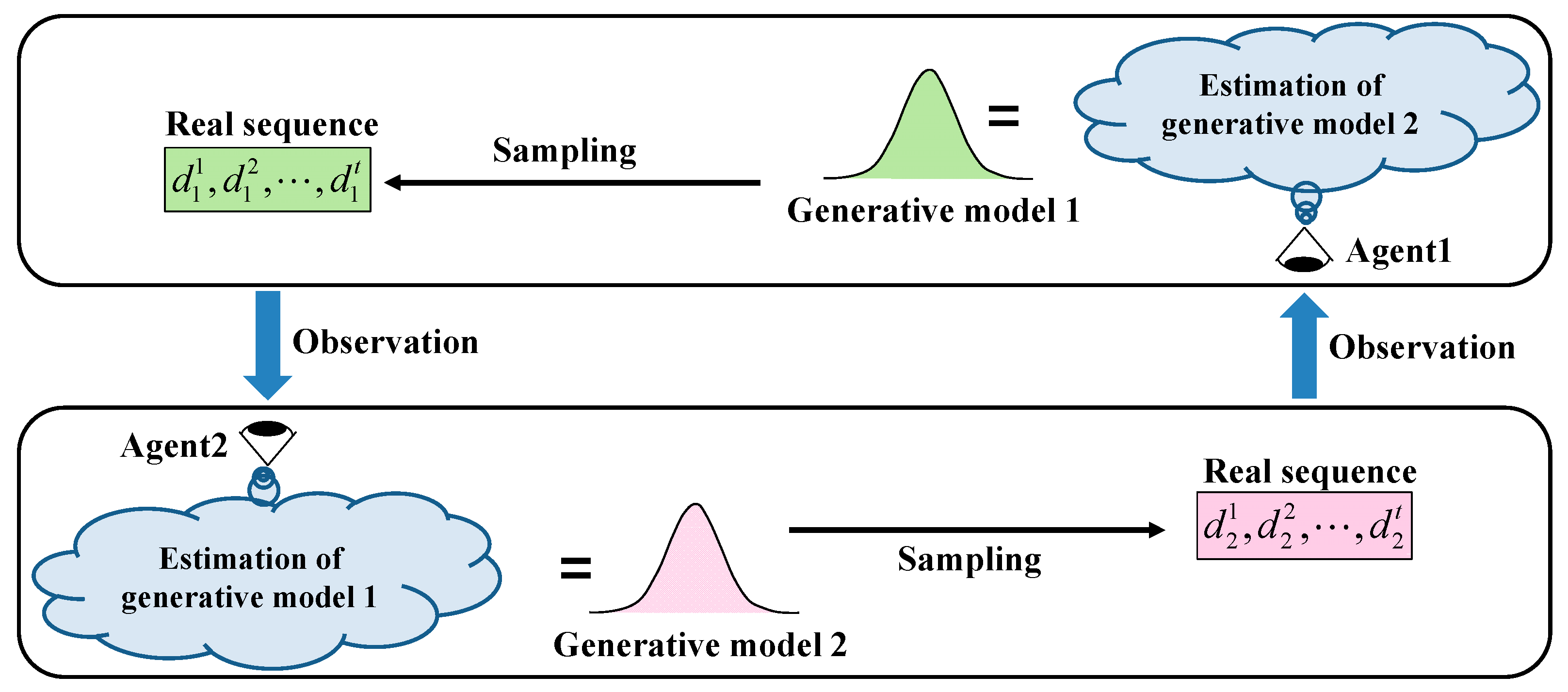
As a minimal model of a non-stationary environment, we consider an imitation game with two decision-making agents (Agents 1 and 2), as shown in Figure 1. This is a game in which each agent estimates the other’s internal state; one can be regarded as the environment of the other. In the imitation game, the target of estimation for each agent is the generative model of the opponent, which changes over time depending on the estimation status of the agent and its opponent. We analyse the behaviour of the agents by running simulations of this game with different forgetting and learning rates.
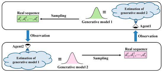
Figure 1.
Outline of imitation game with two decision-making agents using Bayesian inference. First, each agent estimates the generative model of the partner agent from the observation data and uses it as its own generative model. Next, each agent samples a real number from its own generative model and presents it to the other party. The agents repeat these procedures in each step.
Let be the agent’s hypotheses. That is, the total number of hypotheses is . The initial value of confidence for each hypothesis is set to an equal probability, i.e., . The generative model for each hypothesis is a normal distribution, and the variance of the normal distribution was fixed at 0.25, and only the mean value was estimated from the observed data. The initial value of the mean of each model was set to such that these values were equally spaced in the range −0.5 to 0.5.
Each agent samples a real number dt from the generative model of the hypothesis , which it believes most at each time step, and presents it to its opponent. Each agent observes the real number presented by its counterpart and modifies its generative model and confidence values for hypotheses using the extended Bayesian inference described above. The simulation was conducted up to 2000 steps, and the data in the interval of 1000 ≤ t ≤ 2000 was used for the analysis and the display.
The simulation program was developed using C++ language. The compiler was MinGW 8.1.0 64-bit for C++ [26]. The Qt library (Qt version Qt 5.15.2 MinGW 64-bit) was also used for the development [27].
3. Results
3.1. Simulation Results
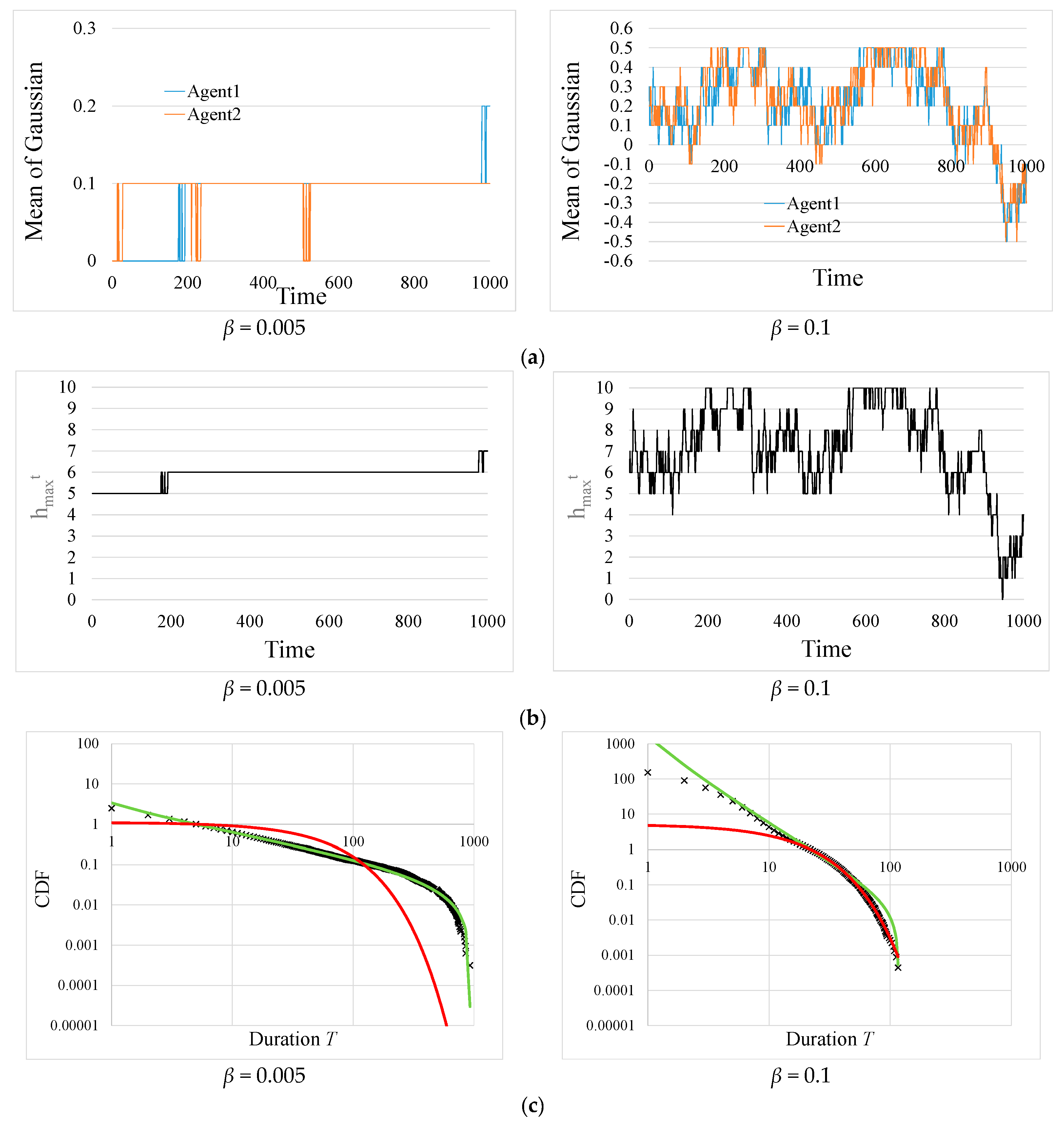
Figure 2 shows the simulation results in the no-learning case (γ = 0.0) with forgetting rates β = 0.005 and β = 0.1. Figure 2a,b show the normal distribution mean value estimated by each agent and the hypothesis that Agent 1 believes most, respectively. Figure 2c shows the cumulative distribution functions (CDF) of T, where T is the time interval from changing at one point to changing at the next point. These figures also show the results of fitting a truncated power law distribution model (green) and an exponential distribution model (red) to the simulation data. Of the observed data, we used only data within the range of to improve the fitting as much as possible. See the SI for details on how we determined the fitting range and the fitting method. The CDF graph is such that the CDF value when is set to ‘1’. This is also true in the following CDF graphs. To analyse the frequency distribution of T, we performed 1000 simulation trials with different random seeds and used the aggregated data. It can be seen from Figure 2c that the frequency distribution of T is characterised by a truncated power law distribution in the case of β = 0.005, while it is characterised by an exponential distribution in the case of β = 0.1. Incidentally, in the case of neither learning nor forgetting, i.e., β = γ = 0.0, over time, the estimates of both agents coincide and becomes invariant. Power laws are found in the narrow parameter region between the invariant and exponential patterns in the case without learning (γ = 0.0).
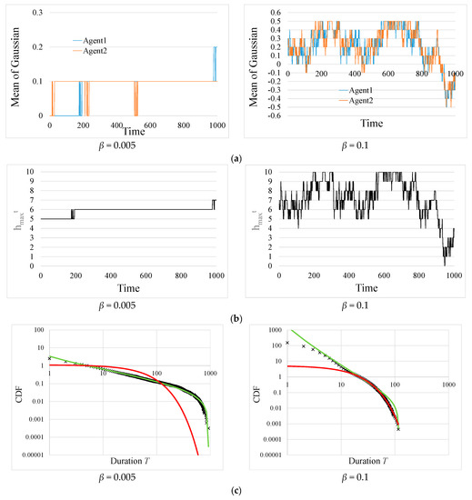
Figure 2.
Results of cases in which the forgetting rate was set to β = 0.005 or 0.1 without learning (γ = 0.0). The left and right columns represent the results in the case of β = 0.005 and the case of β = 0.1, respectively. (a) The time evolution of the normal distribution mean value estimated by each agent. (b) The time evolution of the hypothesis that Agent1 believes the most. (c) Cumulative distribution function (CDF) of duration T of . The exponent of the truncated power law distribution for β = 0.005 was η = 1.58. The exponents of the exponential distribution for β = 0.1 was λ = 0.075. The fitting ranges for β = 0.005 and 0.1 were [5, 927] and [22, 116], respectively.
Figure 3 compares the simulation results for the no-learning case (γ = 0.0) and learning case (γ = 0.1) with forgetting rate β = 0.3. Figure 3a–c shows the normal distribution mean value estimated by each agent, the hypothesis that Agent1 believes most, and Agent1′s confidence in each hypothesis, respectively. In the case without learning (γ = 0.0), the confidence never stays near ‘1’ throughout the simulation period, and changes frequently. On the other hand, we can see that the overall confidence level is higher with the introduction of learning, and that there are periods when the confidence level is almost ‘1’ and is stable.
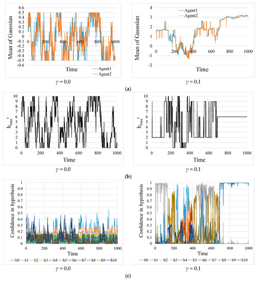
Figure 3.
Examples of time evolution when the forgetting rate β = 0.3. The left and right columns represent the results in the case without learning (γ = 0.0) and the case with learning (γ = 0.1), respectively. (a) The normal distribution mean value estimated by each agent. (b) The hypothesis that Agent1 believes the most. (c) Agent1′s confidence in each hypothesis.
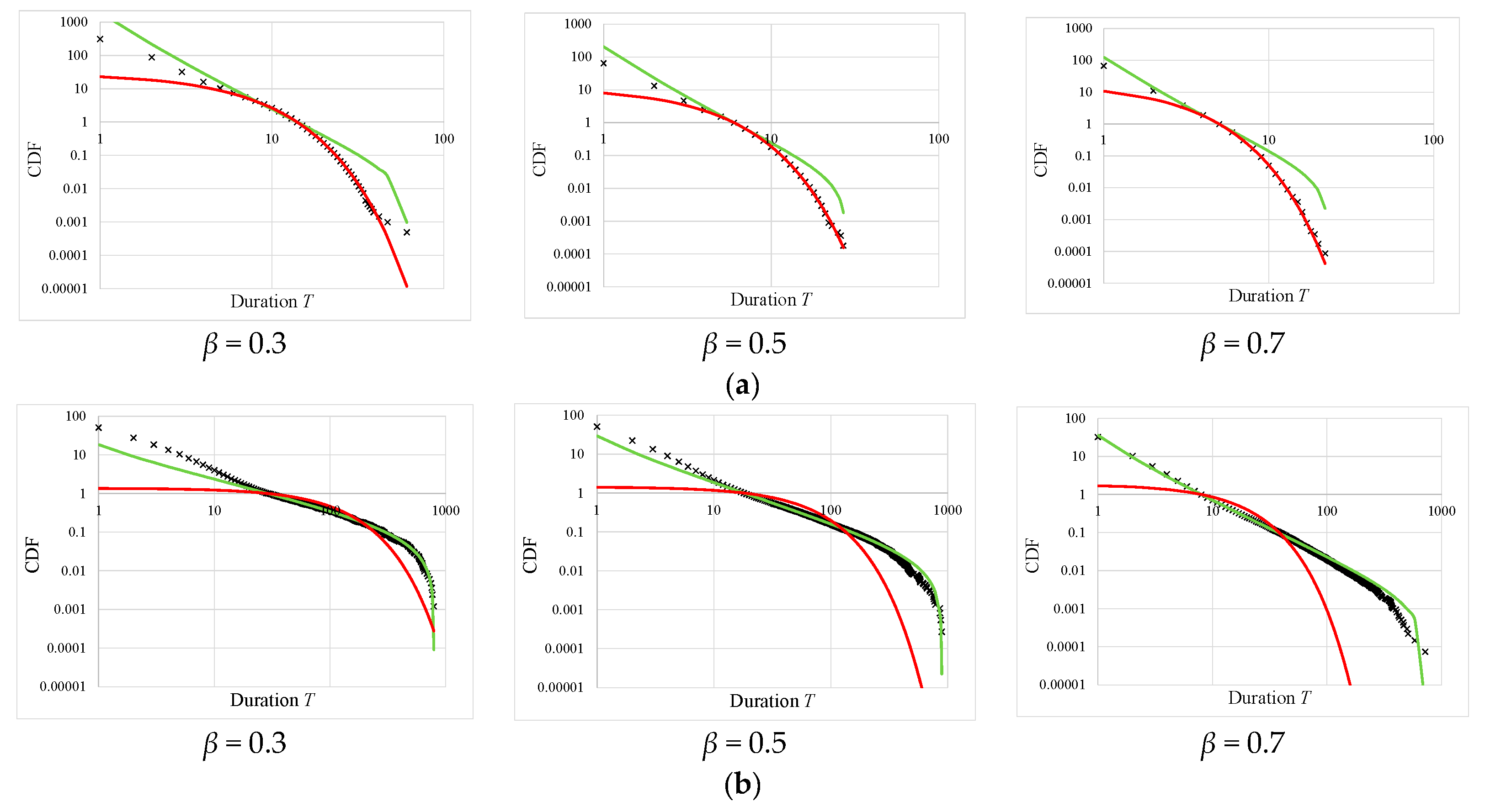
Figure 4a (γ = 0.0) and Figure 4b (γ = 0.1) show the cumulative distribution functions (CDF) of duration T. It can be seen from Figure 4a that the frequency distribution of T is characterised by an exponential distribution. The exponents for β = 0.3, 0.5, and 0.7 were λ = 0.24, 0.42, and 0.60, respectively. The larger β is, the more observational data (information) is truncated, and the larger the value of λ.
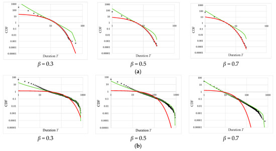
Figure 4.
Results of cases in which the forgetting rate was set to β = 0.3, 0.5, or 0.7. (a) Cumulative distribution function (CDF) of duration T of in the case without learning (γ = 0.0). The exponents of the exponential distribution for β = 0.3, 0.5, and 0.7 were λ = 0.24, 0.42, and 0.60, respectively. The fitting ranges for β = 0.3, 0.5, and 0.7 were [14, 61], [6, 27], and [5, 22], respectively. (b) Cumulative distribution function (CDF) of duration T of in the case with learning (γ = 0.1). The exponents of the truncated power law distribution for β = 0.3, 0.5, and 0.7 were η = 1.73, 2.00, and 2.44, respectively. 1 < η ≤ 3 was satisfied in all cases. The fitting ranges for β = 0.3, 0.5, and 0.7 were [29, 920], [18, 890], and [8, 720], respectively.
Figure 4b shows that the CDF of T is characterised by a truncated power law distribution. The exponents for β = 0.3, 0.5, and 0.7 are η = 1.73, 2.00, and 2.44, respectively, and satisfy 1 < η ≤ 3 in all cases. However, as the forgetting rate increases, the exponents increase because of the information deficit. As can be seen by comparing Figure 4a,b, introducing the effect of learning (inverse Bayesian inference) (γ > 0.0) turns an exponential distribution into a power law distribution.
Originally, the extended Bayesian inference model has a single parameter, as shown in the SI (Supplementary Material) and references [24,25]. That is, we treated only the cases of β = γ and represented these as the same parameter α. Figure 5 shows the CDF of T in the cases of α = 0.3, 0.5, and 0.7. These results represent all power law distributions with the exponents close to 2.0.

Figure 5.
Universally seen power laws. Power laws are found in a wide range of parameter regions; the exponents of the truncated power law distribution are close to 2. (a) α = 0.3, that is, β = γ = 0.3. The exponent of the truncated power law distribution was η = 1.91. The fitting range was [4, 808]. (b) α = 0.5, that is, β = γ = 0.5. The exponent of the truncated power law distribution was η = 1.92. The fitting range was [1, 942]. (c) α = 0.7, that is, β = γ = 0.7. The exponent of the truncated power law distribution was η = 2.10. The fitting range was [4, 970].
3.2. Comparison between with and without Learning
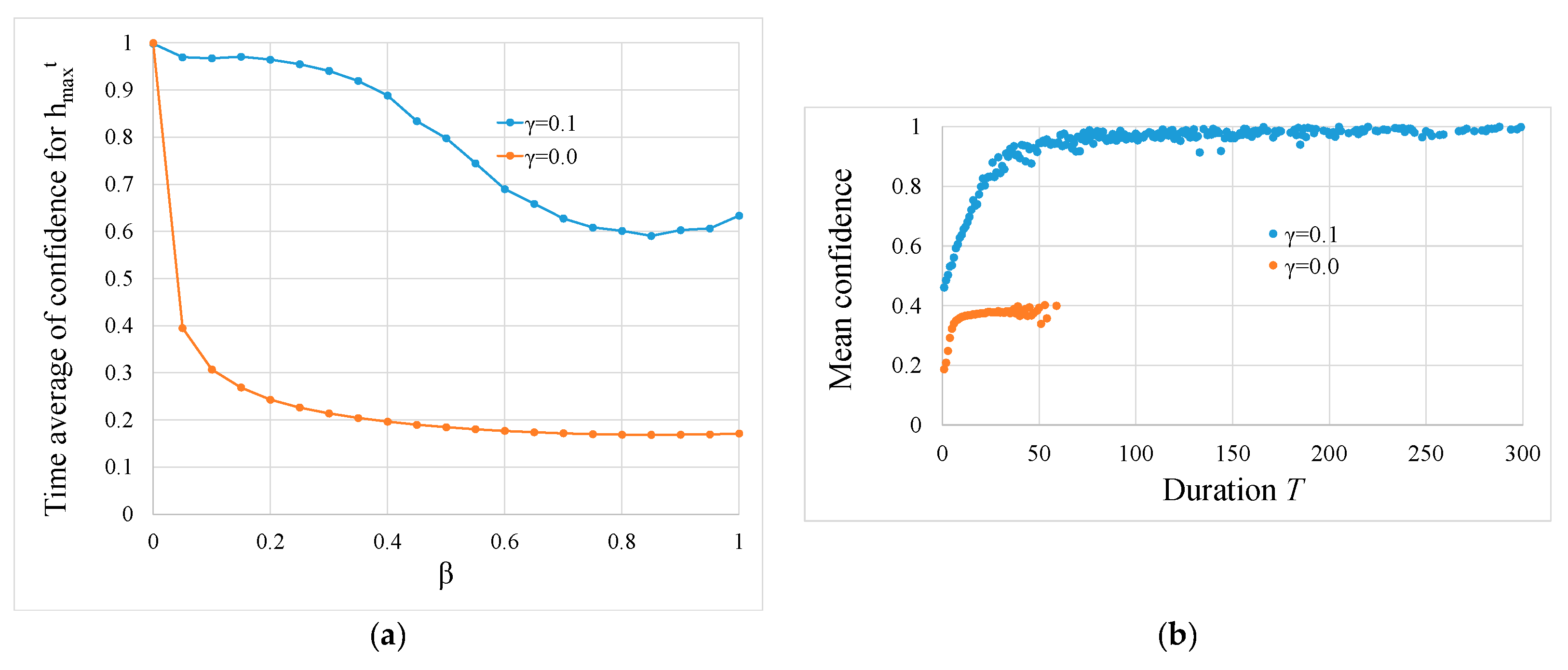
We analysed how confidence changes with changes in forgetting rates. Figure 6a shows the relationship between the time averages of the confidence values in and the forgetting rate. With or without the learning effect, the mean value of confidence decreases as the forgetting rate increases in both cases. In other words, as non-stationarity increases and the amount of information decreases, the confidence decreases. However, a comparison at the same forgetting rate shows that the presence of learning increases the confidence level.
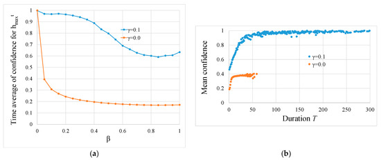
Figure 6.
Comparison between cases with no learning (γ = 0.0) and learning (γ = 0.1). (a) Change in the time average of confidence level with change in the forgetting rate. (b) The relationship between duration T of and confidence (β = 0.3). The vertical axis represents the average confidence during T indicated by the horizontal axis. As the duration increases, the confidence in the hypothesis increases. The duration on the horizontal axis is displayed up to 300 for clarity.
Figure 6b shows the relationship between confidence and duration of . The confidence shown here is the average confidence in the duration of a certain length T. In the absence of learning (γ = 0.0), the maximum duration was 60. The maximum confidence level was approximately 0.40, although it tended to increase as the duration increased. In other words, the confidence level is not very high, and we do not see a long duration. Conversely, in the case with learning (γ = 0.1), the confidence increases as the duration increases, and the confidence exceeds 0.99 when the duration is approximately 300. Thus, agents hypothesize with strong confidence. To calculate the average confidence in Figure 6a,b, we performed 1000 trials of simulations with different random seeds and used the aggregated data.
4. Discussion
In this study we consider the question, ‘What mechanism allows us to be convinced of something even though there is insufficient information for the search target?’ To deal with this problem, we first presented an extended Bayesian inference that introduces forgetting and learning (inverse Bayesian inference) functions into Bayesian inference. We then incorporated this extended Bayesian inference into two decision-making agents and simulated an imitation game in which they read each other’s internal states.
We choose an action from among various options in our daily decision-making, and this choice is accompanied by a degree of certainty. Even if the same action A is selected as a result in different cases, the degree of confidence at the time of selection varies, for example, thinking ‘only A is possible’ or ‘it may be A’. When we lack information and experience, we cannot be sure of our choices. Conversely, when one makes a choice based on complete information, one has confidence in the choice. In other words, the amount of information obtained is proportional to the degree of confidence. However, an action chosen with certainty can actually be wrong. This type of confidence stems from our own active assumptions, rather than objective and complete information. In this study, we model such active assumptions as inverse Bayesian inference.
In stationary environments, Bayesian inference is considered the best method to utilise all information from the distant past to the present. However, for proper estimation in non-stationary environments, it is necessary to discard information about the distant past. In this case, the agent is not sure of its estimation results because of the lack of information. As a result, it frequently changes the estimates, and an exponential distribution appears.
As the lack of information becomes more pronounced, that is, the rate of forgetting increases, the exponent of the exponential distribution that the frequency distribution of the duration of the hypotheses follows increases. By introducing inverse Bayesian inference, the frequency distributions of the duration change from exponential distributions to truncated power law distributions. Interestingly, in the cases where the forgetting rate and the learning rate coincide, over a wide range of parameter areas, the exponents of the truncated power law distributions are close to 2.0, which is the value that achieves optimal foraging behaviour [10].
In inverse Bayesian inference, confidence is increased by modifying the content of the hypothesis to fit the observed data. As shown in Figure 3c and Figure 6a, inverse Bayesian inference (learning) has the effect of increasing the confidence level, and even in situations where there is insufficient information, the confidence level sometimes approaches one. In this case, as shown in Figure 6b, a longer duration tends to correspond to higher confidence.
The simulation of the imitation game in this study could also be performed using a dynamic linear model (DLM) of the state space model [28]. In the DLM, if the covariance of the process noise is larger than that of the observation noise, the Kalman gain is larger; thus, the estimation will focus on more recent data. Accordingly, the forgetting rate may be mapped to the covariance of the process noise or the Kalman gain. The simulation using DLM is a subject for future work.
In the Exploration and Preferential Return (EPR) model, both exploration as a random walk process and the human propensity to revisit places that we have visited before (preferential return) are incorporated. One of these two competing mechanisms is selected probabilistically at each time step in EPR [13]. Exploration and exploitation are two essential components of any optimisation algorithm [29]. Finding an appropriate balance between exploration and exploitation is the most challenging task in the development of any meta-heuristic algorithm because of the randomness of the optimisation process [30]. In our simulations, a power law distribution was produced by a mixture of two competing mechanisms: a long-duration of hypothesis based on confidence and a short-duration of hypothesis estimated while lost. Interestingly, these conflicting patterns of behaviour arise from a single system of extended Bayesian inference without being prepared separately.
As mentioned in the Introduction section, the Levy walk is a type of random walk, with the frequency distribution of the step length as a power law distribution. Wang et al. [31] demonstrated that the frequency distribution of not only the step length but also the duration of stay in a location is a power law distribution in human mobility. In addition, Wang et al. [31] and Rhee et al. [12] demonstrated that the temporal variation of step length is autocorrelated, that is, the temporal variation of step length is time dependent.
Ross et al. [32] demonstrated that in human exploration behaviour, the mode of exploration changes depending on the encounter with the prey. Particularly, they indicated that in response to encounters, hunters produce a more tortuous search of patches of higher prey density and spend more of their search time in patches; however, they adopt more efficient unidirectional, inter-patch movement after failing to encounter prey over a sufficient period.
These findings indicate that human search behaviour is not a random walk, and humans switch their behaviour based on some type of decision-making through interactions with the outside world. In this study, we demonstrated that in a non-stationary environment, the learning and reasoning function intermittently induces a stable mode in which the confidence in a particular hypothesis is nearly 1.0, along with an unstable mode in which the confidence in each hypothesis is low and the hypothesis changes frequently. In the unstable mode, the hypothesis itself changes sequentially, whereas in the stable mode, the hypothesis is fixed and the content of the hypothesis is slightly modified to fit the observed data.
Our proposed model could be one of the models for switching between decision-making modes based on confidence. In the future, we would like to perform simulations in which such switching of the decision-making mode is reflected in the search behaviour and investigate the frequency distribution of step length and the time dependence of step length change.
Namboodiri et al. [11] showed through experiments with humans that the discount rate (forgetting rate) plays an important role in search behaviour. As shown in Figure 2, time-varying patterns of a hypothesis with maximum confidence are characterised by forgetting rates in our model. When the forgetting rate is zero, there is no information loss, and the hypothesis is invariant based on beliefs grounded in complete information. Conversely, when the forgetting rate is high, the estimation results (the hypothesis with maximum confidence) fluctuate because the information is truncated, and the confidence level decreases. As a result, the frequency distribution of the duration of the hypothesis with maximum confidence becomes exponential, as shown in Figure 4a. Power law distributions, which combine both properties, appear in the parameter region between the invariant and the exponential patterns (Figure 2c).
Abe [33] constructed a model in which the Lévy walk appears by coupling two tent maps. In this model, the coupling strength between the two tent maps is represented by the parameter ε. For large values of ε, the output values and of the two coupling tent maps become identical, and the movement pattern in the two-dimensional coordinates becomes a straight line. Conversely, when ε is small, these move independently, and the movement pattern is a Brownian walk. A Lévy walk appears in a narrow parameter range between the two extremes.
In our model, when the forgetting rate is small, the estimates between the two agents tend to agree and have higher confidence as they acquire more information about each other. In contrast, when the forgetting rate is high, the confidence is lowered due to the lack of information about the other party, and inconsistency occurs between the two estimates. Thus, the forgetting rate can be interpreted as a parameter representing the coupling strength between two agents. A simple comparison is not possible because of the difference between tent maps and Bayesian inference. However, we may be able to discuss self-organising criticality (SOC) in our model, as Abe did, by mapping β to ε. In the case of SOC, power laws (Lévy walks) are found in a very narrow parameter range. Hence, in order to explain the universality of power laws found in nature, it is necessary to explain why such parameter regions are selected. Abe attributed this phenomenon to the large dynamic range [33]. In contrast, in our model, power laws are universally found in a wide range of forgetting rate regions by introducing inverse Bayesian inference (learning). That is, in our model, the argument for SOC is only valid in the special case where the learning rate is γ = 0.0. Using a swarm model incorporating BIB inference, Gunji et al. showed that critical phenomena universally emerge without SOC [22]. In this model, critical behaviour is achieved not only at the edge of chaos but anywhere in the parameter space. Detailed discussions on SOC using our model will be had in the future.
5. Conclusions
We presented an algorithm that introduced the effects of learning and forgetting into Bayesian inference, which was proposed by Shinohara et al. [24,25], and simulated an imitation game between decision-making agents that incorporated the algorithm.
In the case of only forgetting without learning, confidence level in one’s chosen hypothesis remained low due to a lack of the other party information, and frequently changed the estimation results. As a result, exponential distributions were observed in a wide range of forgetting-rate areas.
In the case of neither forgetting nor learning, the other party information was not truncated, so that the confidence level remained high based on the complete information and the hypothesis became invariant. Power law appeared only in forgetting rate regions near zero. Conversely, when learning was introduced, power law distributions emerged universally in a wide range of parameter areas by the mixture of high- and low-confidence states. It may be said that the conviction here is not based on complete information, but on active conjecture.
In this paper, we showed that in a non-stationary environment, this kind of active conjecture intermittently induces a stable mode in which the hypothesis is fixed, and the content of the hypothesis is slightly modified to fit the observed data; this is an unstable mode in which the hypothesis itself is changed sequentially. Our proposed model may provide a model for the switching of behavioural modes in human exploratory behaviour.
One limitation of our simulation is that it was conducted with only two agents. In the future, we aim to run simulations with a large number of decision-making agents to analyse their behaviour in a group.
Supplementary Materials
The following are available online at https://www.mdpi.com/article/10.3390/sym13040718/s1.
Author Contributions
Conceptualization, S.S., N.M., Y.N., Y.P.G., T.M., H.O., S.M. and U.-i.C.; formal analysis, S.S.; writing—original draft preparation, S.S.; Writing—Review & Editing, S.S., N.M., Y.N., Y.P.G., T.M., H.O., S.M. and U.-i.C.; Methodology, S.S.; Software, S.S.; Validation, S.S.; Investigation, S.S.; Visualization, S.S.; Supervision, U.-i.C. All authors have read and agreed to the published version of the manuscript.
Funding
This research was supported by the Centre of Innovation Program from the Japan Science and Technology Agency, JST and by JSPS KAKENHI Grant Numbers JP16K01408.
Institutional Review Board Statement
Not applicable.
Informed Consent Statement
Not applicable.
Data Availability Statement
The datasets generated during and/or analysed during the current study are available from the corresponding author on reasonable request.
Conflicts of Interest
The SoftBank Robotics Group Corp. provided support in the form of a salary for author N.M., but did not have any additional role in the study design, data collection and analysis, decision to publish, or preparation of the manuscript. The other authors declare no competing interests.
References
- Harris, T.H.; Banigan, E.J.; Christian, D.A.; Konradt, C.; Wojno, E.D.T.; Norose, K.; Wilson, E.H.; John, B.; Weninger, W.; Luster, A.D.; et al. Generalized Lévy walks and the role of chemokines in migration of effector CD8+ T cells. Nature 2012, 486, 545–548. [Google Scholar] [CrossRef]
- Ariel, G.; Rabani, A.; Benisty, S.; Partridge, J.D.; Harshey, R.M.; Be’Er, A. Swarming bacteria migrate by Lévy Walk. Nat. Commun. 2015, 6, 8396. [Google Scholar] [CrossRef] [PubMed]
- Shokaku, T.; Moriyama, T.; Murakami, H.; Shinohara, S.; Manome, N.; Morioka, K. Development of an automatic turntable-type multiple T-maze device and observation of pill bug behavior. Rev. Sci. Instrum. 2020, 91, 104104. [Google Scholar] [CrossRef]
- Humphries, N.E.; Queiroz, N.; Dyer, J.R.M.; Pade, N.G.; Musyl, M.K.; Schaefer, K.M.; Fuller, D.W.; Brunnschweiler, J.M.; Doyle, T.K.; Houghton, J.D.R.; et al. Environmental context explains Lévy and Brownian movement patterns of marine predators. Nature 2010, 465, 1066–1069. [Google Scholar] [CrossRef] [PubMed]
- Humphries, N.E.; Weimerskirch, H.; Queiroz, N.; Southall, E.J.; Sims, D.W. Foraging success of biological Lévy flights recorded in situ. Proc. Natl. Acad. Sci. USA 2012, 109, 7169–7174. [Google Scholar] [CrossRef] [PubMed]
- Raichlen, D.A.; Wood, B.M.; Gordon, A.D.; Mabulla, A.Z.P.; Marlowe, F.W.; Pontzer, H. Evidence of Lévy walk foraging patterns in human hunter–gatherers. Proc. Natl. Acad. Sci. USA 2014, 111, 728–733. [Google Scholar] [CrossRef] [PubMed]
- Sims, D.W.; Southall, E.J.; Humphries, N.E.; Hays, G.C.; Bradshaw, C.J.A.; Pitchford, J.W.; James, A.; Ahmed, M.Z.; Brierley, A.S.; Hindell, M.A.; et al. Scaling laws of marine predator search behaviour. Nature 2008, 451, 1098–1102. [Google Scholar] [CrossRef] [PubMed]
- Viswanathan, G.M.; Raposo, E.P.; da Luz, M.G.E. Lévy flights and superdiffusion in the context of biological encounters and random searches. Phys. Life Rev. 2008, 5, 133–150. [Google Scholar] [CrossRef]
- Bartumeus, F.; da Luz, M.G.E.; Viswanathan, G.M.; Catalan, J. Animal search strategies: A quantitative random-walk analysis. Ecology 2005, 86, 3078–3087. [Google Scholar] [CrossRef]
- Viswanathan, G.M.; Buldyrev, S.V.; Havlin, S.; Da Luz, M.G.E.; Raposo, E.P.; Stanley, H.E. Optimizing the success of random searches. Nature 1999, 401, 911–914. [Google Scholar] [CrossRef] [PubMed]
- Namboodiri, V.M.; Levy, J.M.; Mihalas, S.; Sims, D.W.; Hussain Shuler, M.G. Rationalizing spatial exploration patterns of wild animals and humans through a temporal discounting framework. Proc. Natl. Acad. Sci. USA 2016, 113, 8747–8752. [Google Scholar] [CrossRef]
- Rhee, I.; Shin, M.; Hong, S.; Lee, K.; Kim, S.J.; Chong, S. On the Levy-Walk Nature of Human Mobility. IEEE ACM Trans. Netw. 2011, 19, 630–643. [Google Scholar] [CrossRef]
- Pappalardo, L.; Rinzivillo, S.; Simini, F. Human Mobility Modelling: Exploration and Preferential Return Meet the Gravity Model. Procedia Comput. Sci. 2016, 83, 934–939. [Google Scholar] [CrossRef]
- Boyer, D.; Ramos-Fernández, G.; Miramontes, O.; Mateos, J.L.; Cocho, G.; Larralde, H.; Ramos, H.; Rojas, F. Scale-free foraging by primates emerges from their interaction with a complex environment. Proc. R. Soc. B 2006, 273, 1743–1750. [Google Scholar] [CrossRef] [PubMed]
- Peirce, C.S. Reasoning and the Logic of Things: The Cambridge Conferences Lectures of 1898; Ketner, K.L., Ed.; Harvard University Press: Cambridge, MA, USA, 1992. [Google Scholar]
- Eco, U.; Sebeok, T.A. (Eds.) The Sign of Three: Dupin, Holmes, Peirce; Indiana University Press: Bloomington, IN, USA, 1988. [Google Scholar]
- Arecchi, F. Phenomenology of consciousness: From apprehension to judgment. Nonlinear Dyn. Psychol. Life Sci. 2011, 15, 359–375. [Google Scholar] [PubMed]
- Zaki, S.R.; Nosofsky, R.M. A high-distortion enhancement effect in the prototype-learning paradigm: Dramatic effects of category learning during test. Mem. Cogn. 2007, 35, 2088–2096. [Google Scholar] [CrossRef] [PubMed][Green Version]
- Zhu, X.; Goldberg, A.B. Introduction to semi-supervised learning; Morgan Claypool: San Rafael, CA, USA, 2009. [Google Scholar] [CrossRef]
- Gunji, Y.P.; Shinohara, S.; Haruna, T.; Basios, V. Inverse Bayesian inference as a key of consciousness featuring a macroscopic quantum logical structure. Biosystems 2016, 152, 44–65. [Google Scholar] [CrossRef] [PubMed]
- Gunji, Y.P.; Murakami, H.; Tomaru, T.; Basios, V. Inverse Bayesian inference in swarming behaviour of soldier crabs. Phil. Trans. R. Soc. A 2018, 376, 20170370. [Google Scholar] [CrossRef] [PubMed]
- Gunji, Y.P.; Kawai, T.; Murakami, H.; Tomaru, T.; Minoura, M.; Shinohara, S. Lévy Walk in swarm models based on Bayesian and inverse Bayesian inference. Comput. Struct. Biotechnol. J. 2020. [Google Scholar] [CrossRef]
- Horry, Y.; Yoshinari, A.; Nakamoto, Y.; Gunji, Y.P. Modeling of decision-making process for moving straight using inverse Bayesian inference. Biosystems 2018, 163, 70–81. [Google Scholar] [CrossRef] [PubMed]
- Shinohara, S.; Manome, N.; Suzuki, K.; Chung, U.-I.; Takahashi, T.; Gunji, P.-Y.; Nakajima, Y.; Mitsuyoshi, S. Extended Bayesian inference incorporating symmetry bias. Biosystems 2020, 190, 104104. [Google Scholar] [CrossRef]
- Shinohara, S.; Manome, N.; Suzuki, K.; Chung, U.-I.; Takahashi, T.; Okamoto, H.; Gunji, Y.P.; Nakajima, Y.; Mitsuyoshi, S. A new method of Bayesian causal inference in non-stationary environments. PLoS ONE 2020, 15, e0233559. [Google Scholar] [CrossRef] [PubMed]
- Available online: http://www.mingw.org/ (accessed on 23 January 2021).
- Available online: https://www.qt.io/ (accessed on 23 January 2021).
- Bishop, C.M. Pattern Recognition and Machine Learning; Springer: New York, NY, USA, 2011. [Google Scholar]
- Emary, E.; Zawbaa, H.M. Impact of chaos functions on modern swarm optimizers. PLoS ONE 2016, 11, e0158738. [Google Scholar] [CrossRef]
- Wu, X.; Zhang, S.; Xiao, W.; Yin, Y. The exploration/exploitation tradeoff in whale optimization algorithm. IEEE Access 2019, 7, 125919–125928. [Google Scholar] [CrossRef]
- Wang, X.W.; Han, X.P.; Wang, B.H. Correlations and Scaling Laws in Human Mobility. PLoS ONE 2014, 9, e84954. [Google Scholar] [CrossRef]
- Ross, C.T.; Winterhalder, B. Evidence for encounter-conditional, area-restricted search in a preliminary study of Colombian blowgun hunters. PLoS ONE 2018, 13, e0207633. [Google Scholar] [CrossRef]
- Abe, M.S. Functional advantages of Lévy walks emerging near a critical point. Proc. Natl. Acad. Sci. USA 2020, 117, 24336–24344. [Google Scholar] [CrossRef]
Publisher’s Note: MDPI stays neutral with regard to jurisdictional claims in published maps and institutional affiliations. |
© 2021 by the authors. Licensee MDPI, Basel, Switzerland. This article is an open access article distributed under the terms and conditions of the Creative Commons Attribution (CC BY) license (https://creativecommons.org/licenses/by/4.0/).

