Article

Machine-Learning Based Memory Prediction Model for Data Parallel Workloads in Apache Spark

Department of Computer Science, Korea University, Seoul 02841, Korea
*
Author to whom correspondence should be addressed.
Symmetry 2021, 13(4), 697; https://doi.org/10.3390/sym13040697
Submission received: 5 March 2021 / Revised: 12 April 2021 / Accepted: 13 April 2021 / Published: 16 April 2021
(This article belongs to the Section Computer)

Abstract

:
A lack of memory can lead to job failures or increase processing times for garbage collection. However, if too much memory is provided, the processing time is only marginally reduced, and most of the memory is wasted. Many big data processing tasks are executed in cloud environments. When renting virtual resources in a cloud environment, it is necessary to pay the cost according to the specifications of resources (i.e., the number of virtual cores and the size of memory), as well as rental time. In this paper, given the type of workload and volume of the input data, we analyze the memory usage pattern and derive the efficient memory size of data-parallel workloads in Apache Spark. Then, we propose a machine-learning-based prediction model that determines the efficient memory for a given workload and data. To determine the validity of the proposed model, we applied it to data-parallel workloads which include a deep learning model. The predicted memory values were in close agreement with the actual amount of required memory. Additionally, the whole building time for the proposed model requires a maximum of 44% of the total execution time of a data-parallel workload. The proposed model can improve memory efficiency up to 1.89 times compared with the vanilla Spark setting.

1. Introduction

Big data analysis applications [1] are executed on distributed parallel processing environments, where multiple worker nodes can perform tasks simultaneously by partitioning big data into multiple blocks. This reduces the time required to perform large amounts of computations. The Hadoop MapReduce framework [2], the first-generation distributed parallel processing platform, performs large-scale computations on big data using a mapping phase that processes parallelizable tasks and a reducing phase that merges results from the mapping phase. A second-generation platform called Apache Spark [3] increases the degree of freedom for designing and implementing big data applications by specifying distributed parallel processing models for applications based on directed acyclic graphs (DAGs). Spark provides a wide range of libraries for various types of workload, such as machine learning [4], streaming data processing [5], and query processing [6] in distributed environments, as well as the existing MapReduce-based algorithms. Overall, it is improving on many aspects of the first-generation platforms. Additionally, it has unique capabilities in terms of performance based on in-memory computing, and resilient distributed dataset (RDD)-based fault tolerance [7].
Most distributed systems for working with big data are implemented on cloud platforms [8]. Cloud service providers lend computing resources to users according to pay-as-you-go policies and charge usage fees accordingly. Therefore, to save the budget, users must select a suitable computing resource for their workload and configure resources efficiently [9,10]. In existing distributed-processing environments, the efficient amount of resources varies depending on the workload type and volume [11]. If these factors are not considered, users may encounter excessive expenditures because of the unnecessary resources or deterioration/failure of the workloads due to insufficient resources. Thus, users must carefully consider the types and amounts of resources suitable for processing their workloads efficiently.
For specifying cloud resources, especially in configuring memory, reducing garbage collection (GC) time is crucial for reducing overall execution time. This is because the time required for memory management is the additional time incurred on top of the actual task processing time [12]. If excessive memory is provided for processing a task, the processing time converges and usage efficiency decreases. Conversely, if too little memory is provided, the total time required to process a workload increases rapidly, which could lead to failure [13].
For the given volume of input data, type of workload, and system environment, it is necessary to consider the features closely related to runtime memory for providing an adequate amount of memory, which enables the workloads to be processed efficiently. Additionally, how the features affect the runtime memory should also be profiled. This paper analyzes the memory usage pattern and derives the efficient memory size of data-parallel workloads in a general distributed environment. We also propose the prediction model for approximating the efficient amount of memory at a low cost for the data-parallel workloads. For predicting the efficient memory size of the workloads accurately, machine learning techniques are adopted. Data characteristics, workload characteristics, and system environment characteristics are used as input features. The main contributions of our study can be summarized as follows.
  • This paper proposes a memory usage model of data-parallel workloads that considers the characteristics of data, workloads, and system environments in the general-purpose distributed-processing Spark platform.
  • Based on the memory usage model, we propose the memory prediction model for estimating efficient amounts of memory of data-parallel workloads using machine learning techniques.
  • When the memory prediction model is applied to data-parallel workloads in the Spark environment, it estimates the appropriate amount of memory at a maximum of 99% accuracy of the actual efficient memory requirements. In terms of cost, efficient memory can be estimated in less than 44% of the workloads’ actual processing time.
The remainder of this paper is organized as follows. The related work and background for this study is provided in Section 2 and Section 3. Section 4 analyzes the memory model and memory usage pattern of Spark. Section 5 analyzes what features affect maximum unrecoverable memory. Section 6 describes the memory estimation model for estimating the amount of required memory by considering the workload type and data size. Section 7 presents the experimental results and performance of the proposed techniques. Section 8 concludes the paper.

2. Related Work

Various studies [14,15,16,17] have been conducted to model big data workload performance. Such studies have selected various features that are considered to be correlated with performance metrics. The metrics are typically measured by varying the values of selected features through tedious experiments. Next, the prediction model that describes the relationship between performance metrics and features is presented. The weights of such a model are trained by exploiting machine learning models. Machine-learning-based models require a priori knowledge for selecting features. Alternatively, additional analysis may be performed to determine which features are directly correlated with metrics. Experiments are typically performed repeatedly to improve the accuracy of a model. The experimental overhead can be significant because of the range and scale of features tested.
In recent years, studies [18,19,20] that predict the performance of workloads based on deep learning have been actively conducted. These studies select features related to the processing time of a workload and train a predictive model with learning data for the features which is the same as that of a machine-learning-based predictive model. Deep learning models generally show higher prediction accuracy than machine learning but have a disadvantage in that the scale of training data is large, and the time required for training is considerable compared to machine learning. The authors of [18] predicted with high accuracy the performance of Spark applications running in a cloud environment using a deep neural network. However, the memory size was not considered as a feature that affects processing time. In [19], a deep fully connected network was used to predict the workload processing time for a number of settings related to the workload’s processing performance, such as Spark. This study reduced the search space for the configuration set through heuristic-based random sampling, thereby reducing the predictive model’s training data collection time. However, it did not consider the impact of the workload’s data characteristics and memory size on the processing time, nor did it consider the efficient memory size for processing the workload. The authors of [20] used a deep neural network to efficiently use computational resources (CPU) in a cloud environment. This study was conducted to maximize the efficiency of computing resources in the cloud by allocating efficient CPU resources when processing Spark and Hadoop MapReduce workloads in the cloud based on marginal utility law. However, this study did not consider the memory size in cloud computing resource configuration and did not consider the data collection time required for deep neural network training. In contrast, our study analyzes the relationships clearly. The relationships provide a basis for the assertion that different workloads have different efficient memory sizes depending on their characteristics and input data. Because the size of memory required for a given workload was predicted with the concrete profile, the number of features used for building the prediction model and samples used for training the model were relatively small compared to previous studies [14,15,16,17,18,19,20]. In this study, it was proven that there is no correlation between the data size of the workload and the unrecoverable memory in order to shorten the training data collection time of the memory prediction model. In the experimental results, it was proven that high prediction accuracy could be achieved by sampling some of the workload’s input data and applying interpolation to the predicted results.
A process running on a Java environment behaves as if the memory it can utilize is infinite. However, allocated memory is typically insufficient when considering the cumulative size of objects created during the runtime [21]. Therefore, a Java virtual machine (JVM) searches for and reserves reusable areas within allocated memory to compensate for memory insufficiency. Such insufficiency occurs when a user provides less memory than the peak memory size required during run time. The amount of time required to reserve recyclable areas varies according to the size of the provided memory. Depending on the workload and size of the input data, the maximum required memory size varies significantly. The memory efficiency depends on the allocated memory size, and the memory size that is actually used. The memory efficiency improvements based on different memory sizes have been researched in a previous study [22]. Other studies have considered efficient memory usage, but they have not been able to predict the specific size of the memory [23,24,25,26]. There have been a few studies on memory prediction in JVM environments [27,28,29]. However, no memory requirement prediction for the Spark environment has been performed.

3. Background

3.1. Data-Parallel Workloads

This section briefly introduces data-parallel model-based big data workloads in the Spark environment. When processing big data or large workloads, data-parallel models are used to support the scalability of data with efficiency. The data-parallel model is suitable for processing big data because multiple worker nodes can independently process data partitions allocated by a master node. When the size of the data or volume of the workload increase, data are distributed to multiple worker nodes and processed in parallel using multi-core processors [30].
The data-parallel model is also used in various machine learning and deep learning model implementations [31,32], which have recently received significant attention. The extensive input data required for training such models can be partitioned and processed simultaneously by multiple worker nodes. As such, the data-parallel model is often used for the distributed parallel processing of large-scale tasks, such as big data processing, machine learning, and deep learning. Therefore, analyzing and modeling data-parallel workloads to improve processing performance is valuable.

3.2. Memory Management Model of the Java Runtime Environment

In an automatic memory management environment, such as Java, a memory management thread independently performs memory allocation and deallocation of the task processing thread (in Java, a memory management thread is called a garbage collector) [33]. Note that since Parallel Old GC is the Spark’s default GC algorithm, the memory management model is described based on the corresponding GC algorithm [34]. Java’s memory model manages the memory by dividing it into multiple areas with different purposes when a process is executed. First, when it is initially executed, all objects created are allocated in the “Eden” space of the “young generation” area. When the Eden space is exhausted, the memory management thread invokes the minor GC procedure. Minor GC pauses all task threads, searches the Eden space, copies the objects that have been connected to root set to the “survivor space” of the young generation area, and frees the memory allocated to the remaining objects. The objects that survive minor GC are determined to be long-term objects that will be used continuously within a process and are migrated to the object space of the “old generation”. Assuming that continuous migrations from the survivor space to the object space happen, major GC occurs when more than a certain percentage of the object space is used. Major GC searches for the object space, removes objects that are unnecessary for processing, and then performs compaction to prevent the fragmentation of empty spaces in the object space. Therefore, major GC generally takes more time than minor GC. When there is insufficient memory to allocate to a new object after major GC, Out-of-Memory Error (OOME) occurs, which causes operations to fail. If OOME occurs during the operation, the entire operation must be redone from the checkpoint, which incurs a considerable cost.

3.3. Data-Parallel Model in Spark

The structure of Spark and the role of each component for implementing data-parallel model in Spark are presented in Figure 1.
The cluster manager [35,36,37] initiates the spark driver on the master node and creates the worker nodes’ executors. Additionally, the cluster manager ensures allocating and retrieving system resources for the Spark driver and executors. Typically, the Spark driver runs on the master node, but it can also run on the client. The Spark driver manages the distributed parallel work processing of executors through SparkContext objects. A worker node is a computing node that manages an executor process that handles actual work. An executor receives the specifications for a job from the driver and processes jobs in parallel using multiple threads.
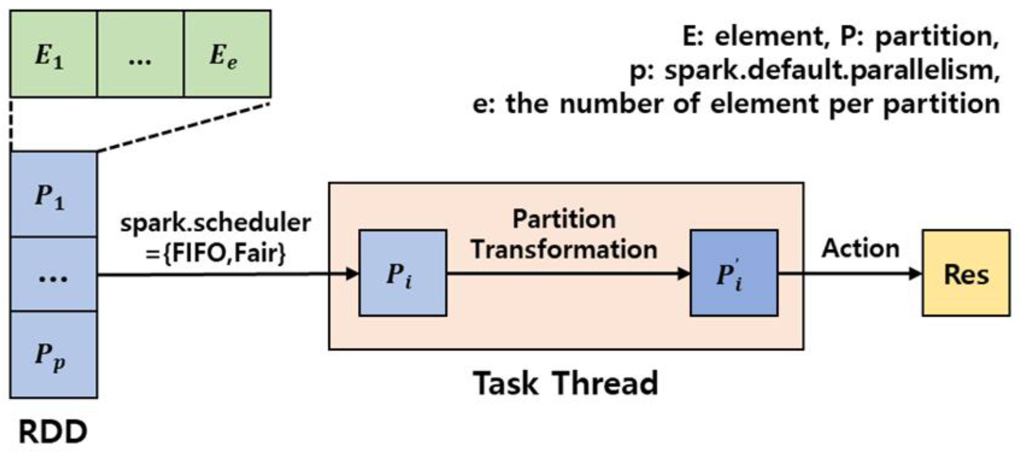
Spark uses an RDD to represent distributed data logically. The Spark driver expresses and processes work in the form of DAGs for RDDs. Figure 2 presents the process for distributed parallel processing of work by executors according to RDD specifications. The RDD is composed of one or more partitions, and each partition is composed of one or more elements. The executor creates threads that fit the parallelism scale specified by the SparkContext and processes the partitions in parallel.
In Spark, transformations and actions are applied to RDD. A transformation applies a user-specified function to all partitions and returns a new type of partitions. Transformations are classified into narrow dependencies with no data exchange among executors and wide dependencies for performing data exchanges. Wide-dependency transformation performs a shuffle operation to exchange data between executors based on key values. Therefore, in a wide-dependency transformation, executors’ amount of required memory varies depending on the distribution state of the key values of the data. An action delivers processed data to the Spark driver, which then outputs the result. This study estimates the appropriate amount of memory required to process a series of big data workloads to exclude overused or underused resources.

4. Spark Memory Model

This section describes how memory is utilized when data-parallel operations are executed in a Spark environment. Furthermore, the memory usage patterns of data-parallel work are described based on the basic operations of Spark.

4.1. Memory Usage Pattern

When a job is submitted to Spark, the Spark driver creates a DAG for the corresponding RDD and requests the RDD’s processing from executors. An executor divides an RDD into partitions and processes partitions in parallel at the thread level. According to the DAG, an executor fetches the partition from a distributed file system [22] or the local file system into the memory to apply a series of transformations to a partition. Whenever a transformation is applied, newly generated partitions are allocated to memory based on Spark’s in-memory processing characteristics. The RDD before the transformation is applied retained by the Spark executor; however, if the executor’s memory runs out, these data are removed. In this case, if the deleted data are required again, the efficiency of in-memory processing decreases because the data must be retrieved from the disk.
Spark provides memory-level or disk-level caching for the reusability of all RDDs. The cached RDDs are retained in the memory until the end of operations. However, if an executor has an insufficient memory, the least-used RDD is deleted according to the default memory management policy for cached RDDs. Therefore, all RDDs are to be removed when the memory allocated by an executor runs out.
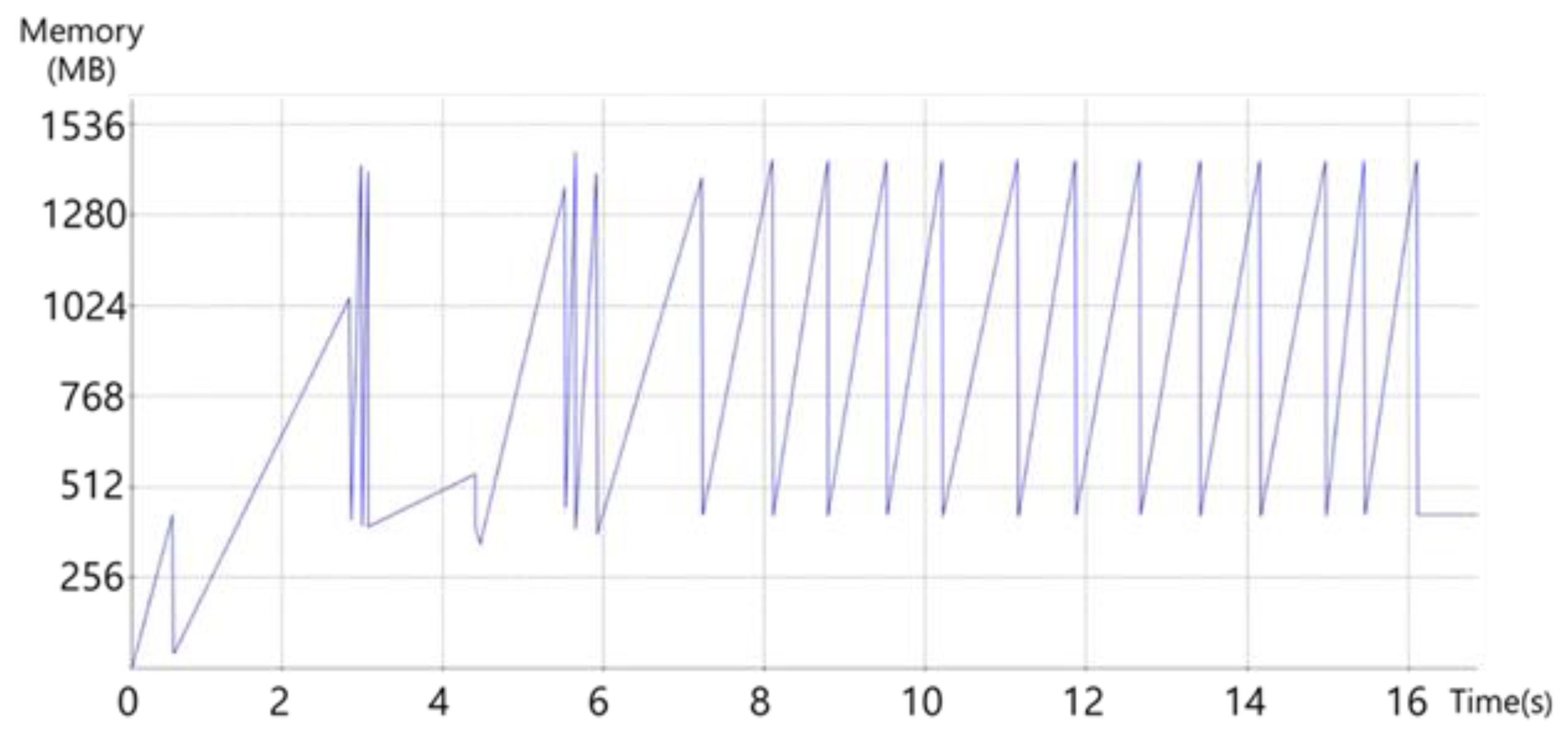
Figure 3 presents an executor’s runtime memory using a Java Flight Recorder when processing a basic transformation map in Spark. The x-axis represents the processing time, and the y-axis represents the runtime memory of the executor. Figure 3 introduces the case when sufficient memory for the target operation is supplied to the executor. If the Eden space reaches a threshold while a workload is being processed, minor GC is performed to secure the recoverable area.
At runtime, objects are created by applying data-parallel operations to partitions. That is, the references to objects can disappear right after a partition is processed. After minor GC, objects still connected to the root set are moved to the survivor space, and the others are removed. After a certain number of minor GCs, remaining objects are moved to the object space. Therefore, only objects located in the survivor space and in the object space are left in the memory following minor GC. Note that when processing the same data-parallel operation for the same input, the runtime memory required after minor GC is almost constant. In Figure 3, after every minor GC, the runtime memory is consistent. It means that the lower limit of the memory required for objects at runtime is fixed. According to Spark architecture, objects created at runtime are classified into two types. The first type is used to process data directly, and the second type performs task management (e.g., communication between the Spark driver and executors during the lifecycle of a workload) [38]. Memory consumption of the first type depends on data characteristics and workload characteristics, and that of the second type depends on system configuration.

4.2. Memory Undersupply

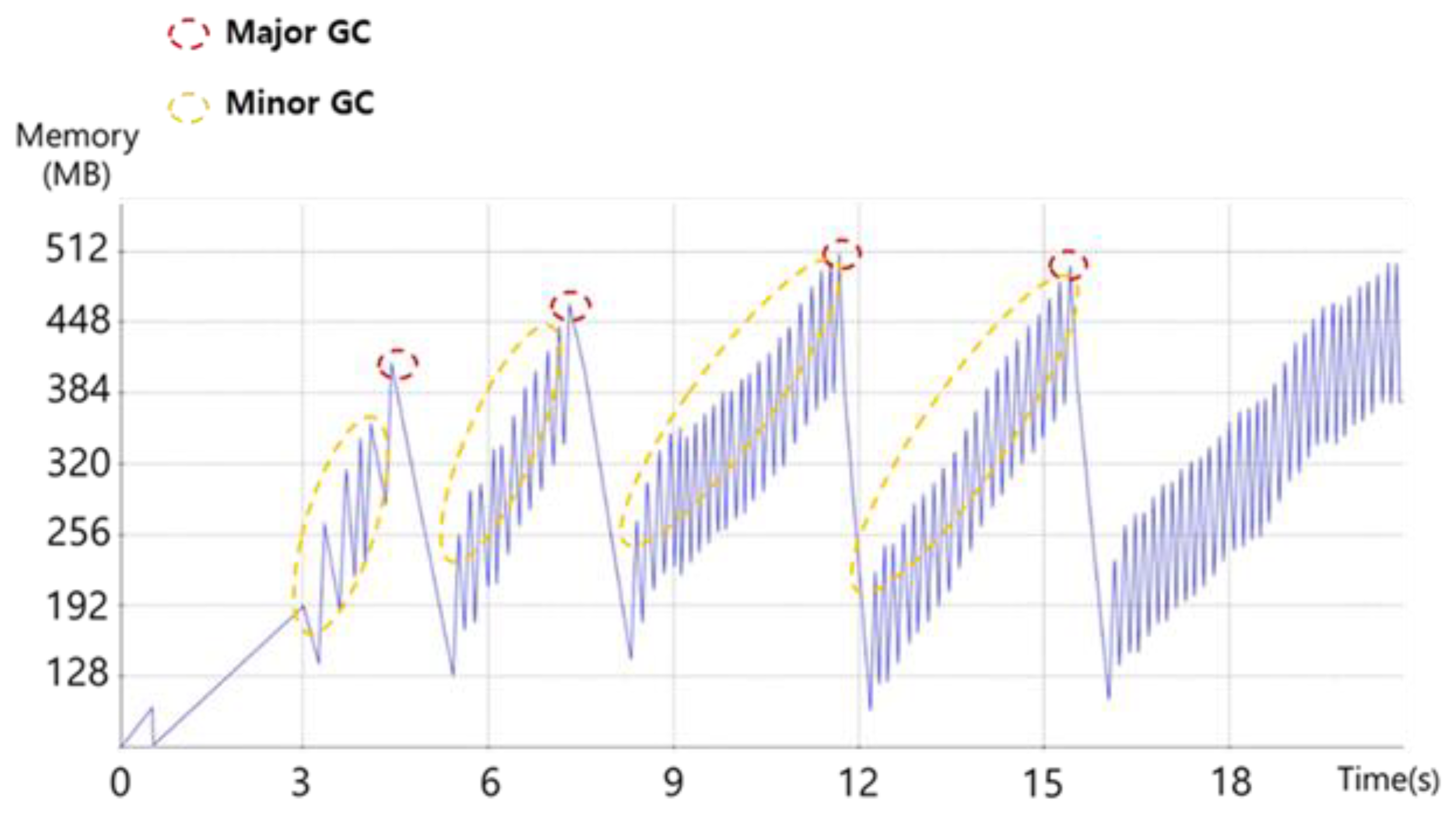
Figure 4 presents runtime memory when the memory is undersupplied. The runtime memory continuously increases after the first minor GC, and the phenomenon occurs repeatedly. When the object space usage reaches the upper threshold, major GC occurs. The major GC rapidly reduces the runtime memory so that the lower bound of runtime memory is near 128MB. It means that the sums of the first- and the second-type objects are nearly consistent. When minor GC occurs, all survived objects should be moved to the survivor space or object space. The objects which survive more than the particular times of minor GCs are migrated to object space. The increased runtime memory after the first minor GC indicates that some objects are abnormally promoted to the object space. Initially, the survived objects in Eden space should be moved to the survivor space. However, when the total size of the surviving objects exceeds the size of the survivor space, some objects should be migrated to the object space. This phenomenon is called premature promotion. In Figure 4, runtime memory increases following minor GC because of continuous premature promotion, which leads to the consumption of object space, causing additional major GCs, thereby increasing the processing time of the workload.
Table 1a shows the percentage of the workloads calculated by dividing the processing time by the lowest processing time when the memory is provided in increments of 0.1 GB from 1 GB to 1.9 GB. The workloads are wordcount, k-means, logistic regression, and neural network. For each memory size, the average processing time was used by performing ten times. In the worst case excepting OOME, at logistic regression with 1.4 GB, the processing time is 1338.7%. Wordcount, which has the smallest difference between the maximum and minimum processing time, has a processing time of 1010.7% compared to the minimum processing time. This proves that even if OOME does not occur, exponential memory management overhead occurs when the memory size is insufficient.

4.3. Memory Oversupply

When memory is oversupplied, only the objects will be migrated to the object space (i.e., the second-type objects), and the others (i.e., the first-type objects) will be removed after minor GC. Since the total size of the object space exceeds the migrated object, no major GC occurs. Consequently, there will be no reduction in the major GC processing, even if excessive memory is provided. Only the trade-off between the number of minor GCs and minor GC processing time occurs. Table 1b shows the percentage of the workloads by dividing the processing time by the lowest processing time when the memory is provided in increments of 1 GB from 2 GB to 11 GB. Wordcount, k-means clustering, logistic regression, neural network algorithms, and convolutional neural network (CNN) are utilized. For each memory size, the average processing time was used by performing ten times. The deviation of processing time for all workloads with different memory sizes is up to 3%. Therefore, providing excessive memory is not cost-effective. This study considers the minimum amount of memory that does not cause the premature promotion to be an efficient amount of memory. Machine learning techniques are used to determine the efficient memory size for a given data-parallel operation. We used data characteristics and workload characteristics that affect runtime memory as input features for the machine learning techniques.

5. Runtime Memory Profiling

In this section, the features considered to affect runtime memory are profiled. First, the impact of the data-parallel model in the Spark environment is profiled. Next, the impact of data representations in Spark and the characteristics of implemented methods are profiled.

5.1. Data-Parallel Characteristics in Spark

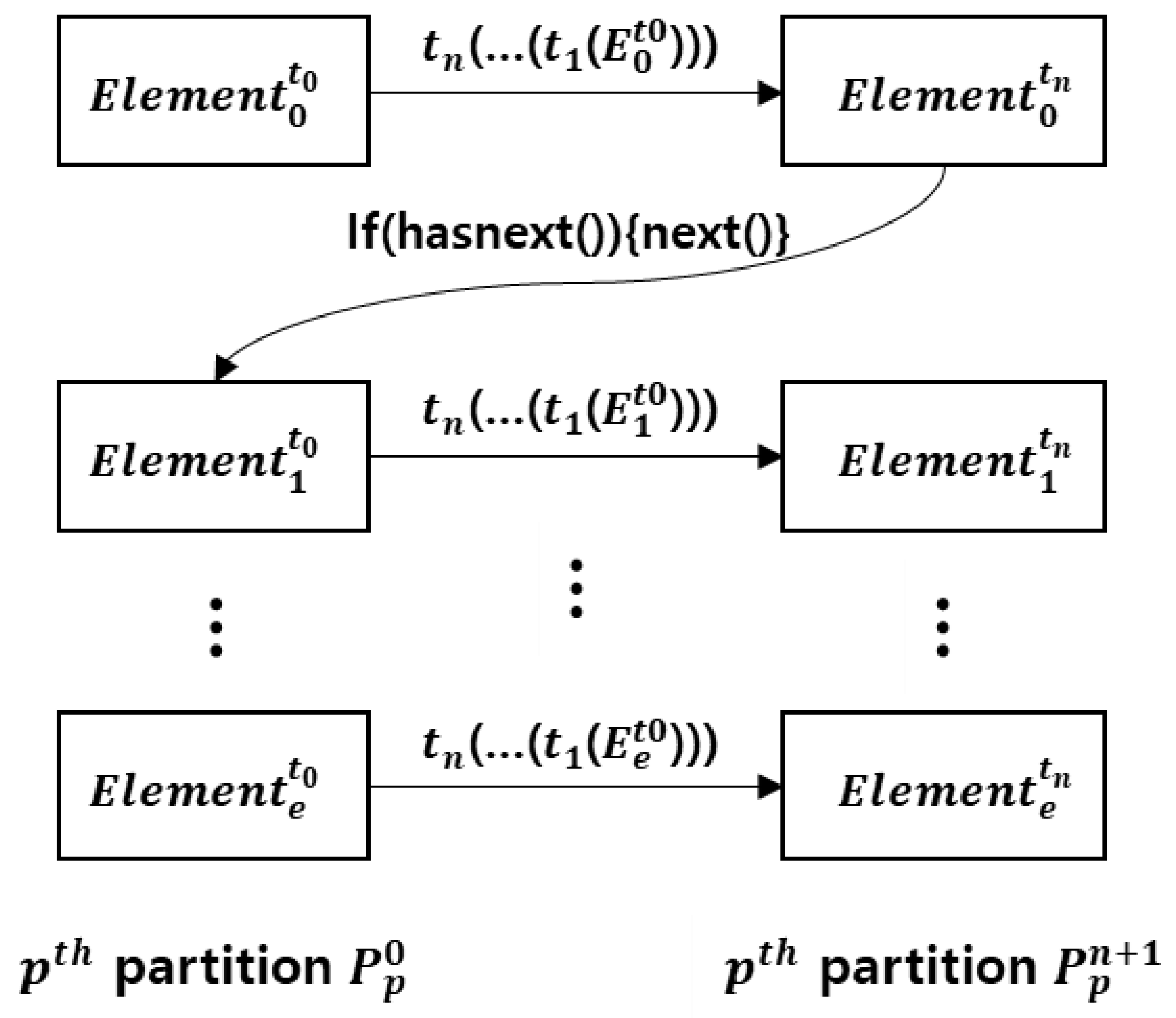
When an action is called, as shown in Figure 5, an executor serially applies transformations (from the first transformation t 1 to the last transformation t n ) to all partitions (from the first partition P a r t i t i o n 0 to the last partition P a r t i t i o n p ) on an element-by-element basis, where p is the index of the partition and the superscript denotes the number of applied transformations. All transformations are applied to all elements from the first element E l e m e n t 0 t 0 , where the subscript denotes the index of the element and t 0 is the recently applied transformation, to the last element E l e m e n t e t 0 . A total of N transformations are applied to all elements. All related notations are described in Table 2.
When applying a series of transformations to an element in Spark, the memory used while applying the previous stage of transformation immediately becomes recoverable. Specifically, when Spark processes data transformation after the previous step’s transformation, the related objects’ references disappear. It means that the associated memory is reclaimed.
A data partition is a collection of elements of any type. Spark implements partitions in the form of iterators. An iterator only has a “next” function that points to the next element and a “hasnext” function that checks the next element’s existence. When applying a transformation to a partition, Spark overwrites the next function with the transformation function. For example, when the Spark “count” action is called, which counts the total number of elements in the result RDD, the next function increments a counter variable after processing one element. For the “collect” action, the results RDD are transformed into an array. Then, the array is transmitted to the driver. Therefore, only the memory used in the transformations applied to the current element becomes unrecoverable memory at runtime.

5.2. Data Characteristics

Data characteristics are the main factors influencing unrecoverable memory during runtime. In Spark, data characteristics are expressed in terms of the element structure and a total number of elements. The total number of elements is expressed as the average number of elements per partition multiplied by the number of partitions. The experiments for Figure 6, Figure 7 and Figure 8 used the average of measurements within 95% of the confidence interval of the unrecoverable memory size as observations after 30 experiments for each variance.
Figure 6 presents the maximum sizes of runtime memory not reclaimed following GC when the number of elements per partition and number of partitions is fixed, and the size of each element increases for the wordcount, k-means, logistic regression, and neural network. For each workload, the unrecoverable memory is measured ten times. In a CNN case, the element size cannot be adjusted because the element structure is a single image. As the element size increases for all workloads, the size of the unrecoverable memory following GC increases. The wordcount has a quasi-linear trend line with an unrecoverable memory size of 111 MB when the element size is 100 KB, and an unrecoverable memory size of 234 MB when the element size is 1000 KB. The k-means algorithm, whose trend line is also quasi-linear, has an unrecoverable memory of 96 MB when the element size is 100 KB, and an unrecoverable memory size of 212 MB when the element size is 1000 KB. Logistic regression exhibits a curved trend with an unrecoverable memory size of 83 MB when the element size is 100 KB, and 240 MB when the element size is 1000 KB. Finally, the neural network algorithm has a linear trend line with an unrecoverable memory size of 83 MB when the element size is 100 KB, and 144 MB when the element size is 1000 KB. Therefore, note that data-parallel operations have different unrecoverable memory depending on the type of operation and size of elements.
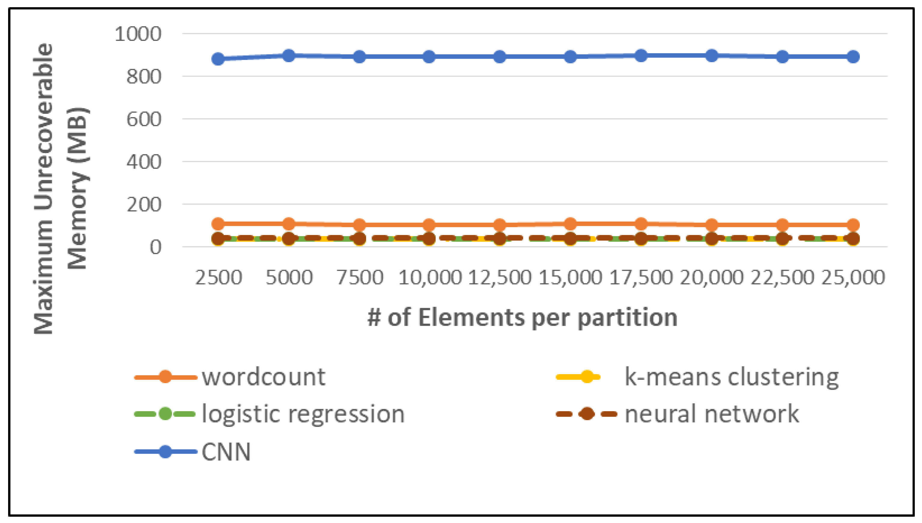
Figure 7 presents the average maximum sizes of unrecoverable memory following GC when the element size and number of partitions are fixed, and the number of elements per partition is increased for the data-parallelized wordcount, k-means, logistic regression, neural network algorithms, and CNN. For each workload, the maximum unrecoverable memory is measured 10 times. As the number of elements per partition increases for all workloads, the size of unrecoverable memory is almost stable. For the wordcount algorithm, the maximum size of unrecoverable memory is 107.797 MB, and the minimum is 106.352 MB. K-means has a maximum value of 37.846 MB and a minimum of 37.421 MB. Logistic regression has a maximum value of 39.646 MB and a minimum of 39.521 MB. The neural network has a maximum value of 41.646 MB and a minimum of 40.796 MB. Finally, CNN has a maximum value of 899.6174 MB and a minimum of 884.126 MB. The size of unrecoverable memory is different for each application; however, it is not affected by the number of elements per partition.
Figure 8 presents the maximum sizes of unrecoverable memory following GC when the size of elements and number of elements per partition are fixed, and the number of partitions is increased for the data-parallelized wordcount, k-means, logistic regression, neural network algorithms, and CNN. Each workload is performed ten times. The maximum size of unrecoverable memory for wordcount is 99.789 MB, and the minimum is 99.042 MB. K-means has a maximum value of 37.846 MB and a minimum of 37.421 MB. Logistic regression has a maximum value of 39.646 MB and a minimum of 37.521 MB. The neural network has a maximum value of 41.646 MB and a minimum of 41.221 MB. Finally, CNN has a maximum value of 894.57 MB and a minimum of 891.275 MB. Similar to Figure 7, the size of unrecoverable memory is different for each workload; however, it is not affected by the number of partitions.

6. Maximum Unrecoverable Memory Estimation

Figure 9 shows the flow diagram for efficient memory size prediction. First, it receives the workload that is the target of memory prediction from the user. The input workload is sent to the Feature Set Collector. The Feature Set Collector sets an element size set, samples the workload’s input data, and executes the workload on the configured element size set and sampled input data. It also measures the maximum unrecoverable memory of the workload while it is running. The result of the Feature Set Collector is delivered to Model Builder. Model Builder creates a model for every combination of the terms in Definition 3. Moreover, it converts Feature Set into Training Data and transfers it to Model Trainer. Finally, Model Trainer trains the transferred data on the received models and then selects the model with the highest prediction accuracy for the test data.

6.1. Estimation Model

For preventing premature promotion, it is necessary to provide an amount of memory greater than the maximum size of unrecoverable memory for a given workload. This section presents a machine-learning-based memory prediction model for predicting the maximum size of unrecoverable memory for a given workload W . A data-parallel workload W is defined in Definition 1.
Definition 1
(Workload). A workload W in Spark is defined by T and a where:
  • T is a finite set of transformation t.
  • a is an action called right after the last transformation.
The maximum unrecoverable memory size required for each transformation and action (i.e., t , a ) is calculated by Definition 2.
Definition 2
(Estimation target). The Maximum Unrecoverable Memory (MUM) of given workload W is Defined as MUM(W) where:
  • For n trials of W, MUM(W) is the maximum value of all runtime memory usages after GC.
Note that the runtime memory usage following GC is measured for all GCs that occur while processing W, and the maximum value of all trials is considered as the maximum unrecoverable memory size. For measuring the runtime memory usage following GC, the “-printHeapatGC” option is used for the executor that observes the target workload. With the option, the memory usage before and after GC is measured for all heap memory areas.
For each W, the relationship between the element size characteristics and MUM(W) is obtained by machine learning models. The unrecoverable memory model for a workload W and related features are defined in Definition 3.
Definition 3
(Estimation model). The estimation model for MUM(W) consists of sum of the terms. Each term is a product of input value based on the size of element (SoE) and model parameter (w). Each term is defined as follows:
  • The first term is bias;
  • The second term is product of SoE multiplied and w 0 ;
  • The third term is product of square root of SoE multiplied and w 1 ;
  • The fourth term is product of logarithm of SoE multiplied and w 2 ;
  • The fifth term is product of square root of SoE and logarithm of SoE and w 3 ;
  • The sixth term is product of logarithm of SoE and SoE and w 4 .
As shown in Definition 3, SoE is the element size of W. Since MUM(W) is only affected by the type of workload and size of elements, it is estimated using features based on SoE. The average number of elements per partition and the number of partitions do not affect MUM(W). Therefore, after generating an unrecoverable memory estimation model, if the workload has the same element structure (i.e., element size), the same model can be reused. Even if the average number of elements per partition and the number of partitions differ, MUM(W) can be estimated accurately. Note that the maximum unrecoverable memory of data-parallel workloads for big data can be estimated using a small amount of data, which significantly reduces the time required to construct the estimation model.

6.2. Model Building Methods

For estimating the maximum unrecoverable memory sizes of a broad range of workloads, the exponential terms and nth power terms of the SoE in Definition 3 can be utilized. However, the use of many weights does not always increase the prediction accuracy. If an estimation model or some features used in such a model are irrelevant, the prediction accuracy is reduced by incorporating additional features. Therefore, only features directly related to memory prediction’s target tasks are selected and used to improve prediction accuracy. Note that, excluding bias, an estimation model was created for all combinations of the remaining set of features in Definition 3. Leave-one-out cross-validation was applied to each estimation model to select the model with the highest prediction accuracy.
In the machine learning models, Lasso regression (Lasso), Ridge regression (Ridge), Random forest (RF), and Multi-layer perceptron (MLP) were used to learn the parameters of the maximum unrecoverable memory prediction model. Therefore, it was necessary to deduce a set of hyperparameters that can maximize the prediction accuracy of performance models. The hyperparameter values applied to each machine learning technique in this study are shown in Table 3, Table 4 and Table 5.
Each table includes a hyperparameter search for each machine learning technique. The hyperparameter set with the lowest mean squared error was used for validation. Lasso and Ridge use L1-norm and L2-norm as penalties to prevent overfitting the training data. The values of Lasso and Ridge used for each hyperparameter are shown in Table 3. Table 4 shows the number of trees (# of estimators) and the values of Max features to increase the accuracy of RF. The Max feature auto enables building a tree using all features, while sqrt and log2 imply building a tree using many features, as these functions are applied to the maximum number of features. The max depth values are also provided to prevent overfitting. In the MLP model, Table 5, a grid search is performed on the combinations of Solver, Activation function, Max iteration (number of training iterations), Learning rate alpha, and the hidden layer’s size to prevent overfitting and under-fitting and to improve prediction accuracy.

7. Experiment

In the first subsection, the experiment environment (e.g., the clusters’ specifications, platform parameters) is described. Next, data-parallel workloads that are used for performance evaluation and their input data are presented. After that, the performance metrics of the maximum unrecoverable memory prediction model are described. Finally, we apply the prediction model for all workloads and present performance for each metric. Additionally, the model’s performance is evaluated for each model building method.

7.1. Experiment Environment

Our experiments were conducted using a cluster of one master and four workers. Each device had an i7-6700 (8 cores, 3.4 GHz) CPU, 16 GB of RAM, a 256 GB SSD, and 1 Gbit of network bandwidth. The Ubuntu 16.04 LTS operating system, Java Runtime Environment version 1.8.0, Spark version 2.1.0, and Scala version 2.11.8 were used to collect the model’s input/output data and to implement the prediction model. In this study, each executor processed a workload with the same specifications and the same amount of data simultaneously. Therefore, the maximum amount of unrecoverable memory for a given workload was the same for all processors. For estimating the maximum amount of unrecoverable memory with a default configuration, the number of cores per processor, initial memory provision, and the number of partitions were set according to Spark’s default settings.

7.2. Performance Metrics

The performance of the proposed memory prediction model was evaluated with three different metrics. The first one is A c c u r a c y , which is calculated as shown in Equation (1), where a n s w e r is the maximum amount of unrecoverable data measured during validation and p r e d i c t e d is the predicted value for a given model based on training data.
A c c u r a c y = | ( a n s w e r p r e d i c t e d ) | a n s w e r 100 %
The second metric is P r e d i c t i o n   C o s t , which is defined as the ratio of the execution time for memory prediction over the total execution time for a workload, as shown in Equation (2). M o d e l   G e n e r a t i o n   T i m e is the whole processing time for building the model. It includes the time for collecting sample data and the time for training the model for each set of element sizes for a given workload. W o r k l o a d   R u n n i n g   T i m e is the workload running time of one validation dataset.
P r e d i c t i o n   C o s t = M o d e l   G e n e r a t i o n   T i m e / W o r k l o a d   R u n n i n g   T i m e 100 %
As shown in Equation (3), E f f i c i e n c y is the third metric. It is calculated by dividing P r o p o s e d   M e m o r y   E f f i c i e n c y by D e f a u l t   M e m o r y   E f f i c i e n c y . As shown in Equation (4), P r o p o s e d   M e m o r y   E f f i c i e n c y is the reciprocal of the product of E x e c u t i o n   T i m e and P r o v i d e d   M e m o r y   p e r   E x e c u t o r when the proposed model’s result is used. D e f a u l t   M e m o r y   E f f i c i e n c y is the reciprocal of the product of E x e c u t i o n   T i m e and P r o v i d e d   M e m o r y   p e r   E x e c u t o r when Spark’s default memory is used.
E f f i c i e n c y = P r o p o s e d   M e m o r y   E f f i c i e n c y / D e f a u l t   M e m o r y   E f f i c i e n c y 100 %
M e m o r y   E f f i c i e n c y = 1 / ( E x e c u t i o n   T i m e P r o v i d e d   M e m o r y   p e r   E x e c u t o r )

7.3. Workload

The proposed memory prediction model was applied to four data-parallel workloads. The details of the workloads are discussed below.

7.3.1. Wordcount

The wordcount algorithm extracts words from a given document set and calculates how many times certain words appear within the documents. The workload consists of tasks that transform the document set into distributed data in the single-line element format. Then, it splits each element into words. Lastly, it calculates the occurrence frequency of different elements within the documents. As a conclusion, the maximum amount of unrecoverable memory was estimated for three transformations called “map,” “flatmap,” and “reducebykey,” which are data-parallel operations.

7.3.2. K-Means Clustering

The k-means clustering [39] algorithm finds the central K points for a given set of vectors. For each vector, a central point closest to the vector is selected, and the vector is included in the point’s group. The central point for each group is selected as a new centroid. Grouping the vectors and selecting new centroids is done recursively while termination conditions are fulfilled. Therefore, the workload consists of a set of transformations that create a k-means clustering model for all elements based on K points and a set of transformations that calculate the silhouette scores for a given dataset. We estimated the maximum amount of unrecoverable memory for these two sets of data-parallel transformations.

7.3.3. Logistic Regression and Neural Network

Logistic regression [40] is an algorithm that derives an objective function representing the correlation between input vectors and output values. Therefore, a set of weights (i.e., model parameters) that can reduce the difference between the regression function’s results and the actual result values is trained. The neural network algorithm [41] is similar to logistic regression, but there is a structural difference in that a neural network contains multiple hidden layers between input vectors and output values. In the neural network, the input layer has been adjusted to match the element sizes in Table 6. Two hidden layers are used, and each consists of 100 neurons. Finally, the output layer used two neurons. A neural network requires greater computational power than logistic regression because it must calculate multiple hidden layers’ weight vectors. The maximum amount of unrecoverable memory was predicted for a data-parallel transformation set that obtains output values by solving logistic functions and another set of transformations that calculates updated weight values.

7.3.4. Convolutional Neural Network (CNN)

The CNN [43] is a deep learning model that mainly receives visual images and processes tasks such as recognition and classification with high accuracy. Similar to the neural network structure, several hidden layers are arranged between the input and output layers. However, there is a structural difference in arranging multiple convolution layers and pooling layers between the input and output layers. Therefore, compared to the neural network, the model is large, and the complexity is high. Since the parallelization of the CNN model (e.g., InceptionV4) is implemented on a partition basis, the maximum value of the unrecoverable memory is predicted for all transformations that output CNN’s result from one image.

7.4. Workload Input Data Description

The workload’s element format and element size are described in Table 6. The wordcount uses documents as an input and the string as an element. The wordcount input documents consist of randomly generated characters. In the implementation, the length of characters is equal to the element size. Since k-means clustering, logistic regression, and neural networks use vectors as input values, the element is a set of real numbers. The element of the workloads consists of randomly generated double-type numbers. The total size of the double-type numbers is equal to the element size. Note that existing datasets cannot be used since the size of the element should be manipulated.
For the wordcount, k-means clustering, logistic regression, and neural network, the minimum element size is 1 KB, and the maximum is 1 MB. This range was divided into seven and ten groups for each workload. The first set is denoted as Element size set1, and the second set is defined as Element size set2. The average of samples within 95% of the confidence interval of the unrecoverable memory size is used as a measurement after repeating 30 experiments for each element size in Table 6. In the CNN case, the element is a single image, so the element size cannot be adjusted. Instead, yelp data [43] were used as input data.
Since the unrecoverable memory is critically affected by element size, only small partitions for each element size were used to train the memory prediction model. However, when verifying the model’s performance, more than 10 GB of data were used to reflect a data size scalability. For each element size, 100 MB of training data were generated. Additionally, 10, 30, 50, and 100 GB of data for each element size were generated as the validation data. In the CNN case, images from the yelp dataset were duplicated for adjusting the total size of input data to be 10, 30, 50, and 100 GB.

7.5. Performance Evaluation

7.5.1. Prediction Accuracy

The experiments for each workload and for each model building method were divided into two cases. The first case trains the model using Element size set1, and the second case utilizes Element size set2. In both cases, models were trained using the result from 100 MB of input data. For each element set, accuracy was calculated using the experiment results of 10, 30, 50, and 100 GB input datasets.
Figure 10 describes when Lasso is applied to both Element size set1 and Element size set2. In Element size set1, k-means clustering with validation data size 100 GB has a minimum accuracy of 94.4%, and neural network with validation data size 10 GB has maximum accuracy of 98.7%. In Element size set2, wordcount with 100 GB have an accuracy of at least 96.3%, and a neural network with 10 GB has an accuracy of up to 99.7%. The average accuracy of more than 95% proves that the polynomial regression machine learning technique effectively predicts the maximum unrecoverable memory of all workloads.
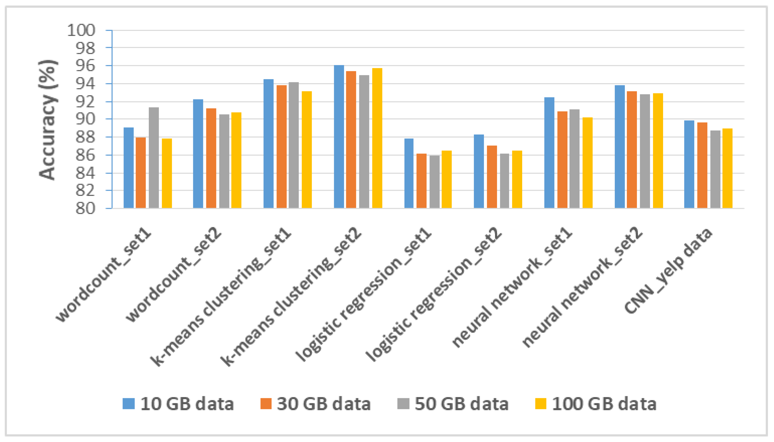
In Figure 11, both Element size set1 and set2 with Ridge are described. When Ridge is applied to Element size set1, the accuracy of at least 85.9% is achieved in logistic regression with 50 GB. In k-means clustering with the validation data size of 10 GB, it has a maximum of 94.5% accuracy. In Element size set2, logistic regression with 50 GB has an accuracy of at least 86.2%, and k-means clustering with 10 GB has a maximum accuracy of 95.7%. Ridge, which has the lowest average prediction accuracy, is also less affected by the workload input data size.
In Figure 12, when RF is applied to Element size set1, logistic regression with validation data size 30 GB has the lowest accuracy of 95.1%, and neural network with validation data size 10 GB has an accuracy of up to 99.4%. Element size set2 achieves at least 96.3% accuracy in logistic regression with validation data size 30 GB. It has an accuracy of up to 99.5% in neural network with validation data size 10 GB. When RF was applied, the average prediction accuracy was the highest for all workloads.
In Figure 13, when MLP is applied to Element size set1, wordcount with validation data size 50 GB has the lowest accuracy of 95.9%. Furthermore, when the size of the validation data in the neural network is 10 GB, it has a maximum accuracy of 98.7%. The Element size set2 has an accuracy of at least 96.2% when the validation data size is 10 GB and 100 GB is applied to logistic regression. It has up to 99% accuracy in neural network when the validation data size is 10 GB. In the case of neural network, the larger the workload input data, the lower the prediction accuracy compared to other techniques due to overfitting problem. As a result, the proposed memory prediction model shows less than 2% accuracy reduction even when the size of the workload’s input data increases. It means that the proposed model guarantees the scalability of the input data size.

7.5.2. Prediction Cost

M o d e l   G e n e r a t i o n   T i m e at Equation (2) is the sum of the time necessary to collect the training data and to build the model with the highest prediction accuracy using the model building method. The training data collection time refers to collecting 100 training samples for all workloads with Element size set1 and set2, excluding CNN. For each element in Element size set1 and set2, 100 MB input data are used to collect a training sample. The number of training samples is sufficient to be utilized in machine-learning-based methods. Note that even with 100 training samples for each case, the prediction accuracy is kept high, but also the prediction cost at Equation (2) is reasonable. W o r k l o a d   R u n n i n g   T i m e at Equation (2) is the total workload execution time when input data are 10 GB and 100 GB. Figure 14, Figure 15 and Figure 16 present the prediction costs when 100 MB of input data are used for each workload, and 100 training samples are used to train the prediction model. The workloads’ prediction costs are validated with 10 GB and 100 GB input data.
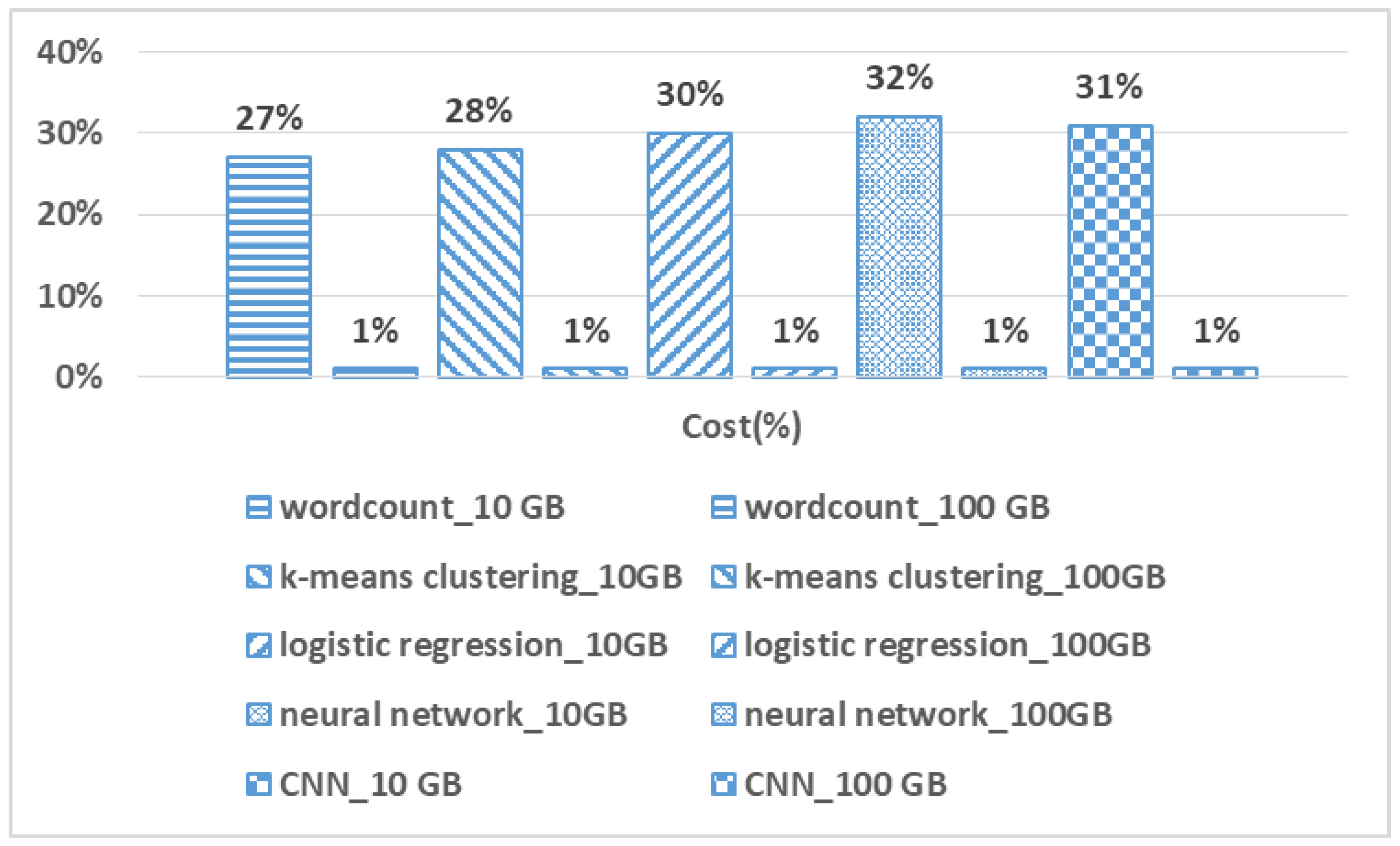
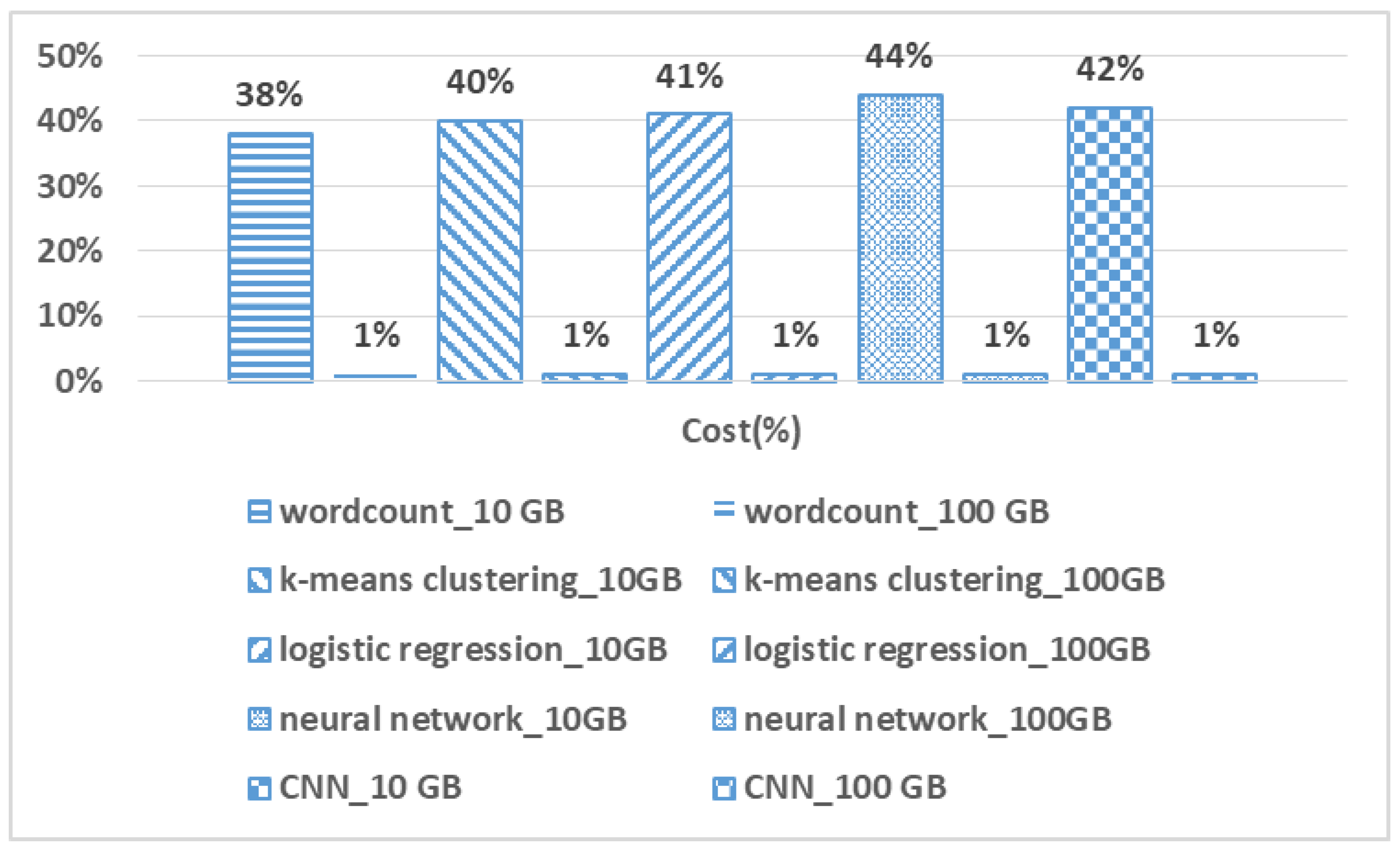
Figure 14 shows the prediction cost for generating Lasso and Ridge regression-based prediction models for all workloads. In Lasso and Ridge’s case, the prediction cost is similar because the processing method is almost the same except for the penalty term. Therefore, the average prediction cost of the two methods was calculated. When the input data are 10 GB, the time required for model generation for each workload is at least 27% in wordcount and at most 32% in the neural network. However, when the input data are 100 GB, it is less than 1% for all workloads. Figure 15 shows the prediction cost when RF is applied to all workloads. When input data are 10 GB, it is at least 23% in wordcount and at most 26% in the neural network. At 100 GB, it is equally less than 1% for all workloads. Finally, Figure 16 shows the prediction cost when MLP is applied. Compared to other gradient descent methods, MLP takes the longest time to create a model because it has the largest hyperparameter space. In addition, as the number of epochs for training data is large, the time required is longer than the others. Therefore, when the input data are 10 GB, it is at least 38% in wordcount and 44% in the neural network. However, if the input data are 100 GB, even if MLP is applied, the prediction cost is less than 1% for all workloads.
Note that as the input data’s size increases, the cost of the proposed technique itself is relatively small because the time required to generate a model is static, and the total processing time is proportional to the size of the input data.

7.5.3. Memory Efficiency

Figure 17 presents E f f i c i e n c y at Equation (3) of whole workloads. For calculating E f f i c i e n c y in Equation (3), D e f a u l t   M e m o r y   E f f i c i e n c y and P r o p o s e d   M e m o r y   E f f i c i e n c y are required. Additionally, for calculating D e f a u l t   M e m o r y   E f f i c i e n c y and P r o p o s e d   M e m o r y   E f f i c i e n c y in Equation (3), both E x e c u t i o n   T i m e and P r o v i d e d   M e m o r y   p e r   E x e c u t o r are required. E x e c u t i o n   T i m e of the former is observed by processing workloads with default memory values of Spark’s standalone cluster for 100 GB validation datasets. P r o v i d e d   M e m o r y   p e r   E x e c u t o r of the former is the default memory values of Spark’s standalone cluster. E x e c u t i o n   T i m e of the latter is observed by processing workloads with result values of our memory prediction model for 100 GB validation datasets. P r o v i d e d   M e m o r y   p e r   E x e c u t o r of the latter is the result values of our predictor. A higher value indicates enhanced memory efficiency. Note that we calculated the memory efficiency based on the prediction model, which has the highest accuracy when the input data size is 100 GB for each workload.
The standalone cluster provides 1 GB of memory to each executor by default. Therefore, a total of 4 GB is allocated so that each worker uses 1 GB equally without generating out-of-memory errors. In the case of CNN, since the minimum memory that does not generate OOME is 8 GB per executor, efficiency is calculated according to the corresponding memory and the predicted memory size. When the proposed method is applied, the efficiency is boosted by at least 1.33 times for CNN and up to 1.89 times for the neural network. The larger the default memory size provided to the executors, the higher the efficiency with the memory derived by the proposed technique.

8. Conclusions

When processing workloads in an in-memory distributed parallel processing environment, efficient memory usage is beneficial in terms of resource usage but is also a challenge. There have been studies to predict efficient memory in the JVM environment, but this did not take into account in-memory-based distributed parallel processing environments such as Hadoop MapReduce and Spark. Since then, there have been papers on performance prediction for efficient workload processing by manipulating parameters related to processing performance based on machine learning or AI in the environment. However, the analysis of how memory causes a causal relationship to the workload processing performance in the environment and studies to derive an efficient memory value has been insufficient. Additionally, the disadvantage of existing machine learning or AI-based predictive models is that the workload must be rerun dozens or hundreds of times to collect data for model training.
This paper proposed a low-cost method for predicting unrecoverable memory size with high accuracy for big data processing data-parallel tasks in a general distributed environment. At first, to define the efficient memory size for a data-parallel operation, data-parallel processing in the distributed platform and memory management overhead in a JVM were analyzed. Secondly, we proposed the prediction that estimates the maximum amount of unrecoverable memory for a given workload at runtime by analyzing memory usage patterns. Thirdly, existing machine learning or deep learning-based models are challenging to use in practice because of the time needed to collect data for training. However, in this study, when the volume of the prediction target workload is large and the time required for model construction is considerable, a small amount of sampled input data is used, and the time required for building the model is reduced through using extrapolation. Additionally, when evaluating the performance of trained memory models, they achieved high prediction accuracy for validation datasets that were much larger than the input data of the training samples. By applying the proposed technique to typical data-parallel workloads, the workloads’ memory efficiency is improved prominently. In future work, we will prove the proposed technique’s effectiveness in other frameworks that perform in-memory distributed parallel processing in the Java environment, such as Hadoop MapReduce framework. Furthermore, based on efficient memory size prediction and workload processing time prediction [44], we will develop a resource recommendation system that can efficiently set operator resources and memory for the target processing time in a configurable resource environment such as docker container [45]. The effectiveness of the system will be proved through statistical tests like [46,47].

Author Contributions

Conceptualization, R.M.; methodology, R.M.; software, R.M.; validation, R.M., S.C.; formal analysis, R.M.; investigation, R.M.; resources, R.M., S.C.; data curation, R.M.; writing—original draft preparation, R.M., S.C.; writing—review and editing, R.M., S.C.; visualization, R.M., S.C.; supervision, S.C.; project administration, S.C.; funding acquisition, S.C. All authors have read and agreed to the published version of the manuscript.

Funding

We thank the anonymous reviewers for their insightful feedback. This work was partly supported by the National Research Foundation of Korea, NRF under grants NRF-2018R1D1A1B07050377. The corresponding author of this paper is Sukyong Choi (Email: csukyung@korea.ac.kr).

Institutional Review Board Statement

Not applicable.

Informed Consent Statement

Not applicable.

Data Availability Statement

Not applicable.

Conflicts of Interest

The authors declare no conflict of interest.

References

  1. Hu, H.; Wen, Y.; Chua, T.S.; Li, X. Toward scalable systems for big data analytics: A technology tutorial. IEEE Access 2014, 2, 652–687. [Google Scholar] [CrossRef]
  2. Dean, J.; Ghemawat, S. MapReduce: Simplified data processing on large clusters. Commun. ACM 2008, 51, 107–113. [Google Scholar] [CrossRef]
  3. Zaharia, M.; Xin, R.S.; Wendell, P.; Das, T.; Armbrust, M.; Dave, A.; Meng, X.; Rosen, J.; Venkataraman, S.; Franklin, M.J.; et al. Apache Spark: A unified engine for big data processing. Commun. ACM 2016, 59, 56–65. [Google Scholar] [CrossRef]
  4. Meng, X.; Bradley, J.; Yavuz, B.; Sparks, E.; Venkataraman, S.; Liu, D.; Freeman, J.; Tsai, D.B.; Amde, M.; Owen, S.; et al. Mllib: Machine learning in apache Spark. J. Mach. Learn. Res. 2016, 17, 1235–1241. [Google Scholar]
  5. Zaharia, M.; Das, T.; Li, H.; Hunter, T.; Shenker, S.; Stoica, I. Discretized streams: Fault-tolerant streaming computation at scale. In Proceedings of the Twenty-Fourth ACM Symposium on Operating Systems Principles; ACM Association for Computing Machinery: New York, NY, USA, 2013; pp. 423–438. [Google Scholar]
  6. Xin, R.S.; Gonzalez, J.E.; Franklin, M.J.; Stoica, I. Graphx: A resilient distributed graph system on Spark. In First International Workshop on Graph Data Management Experiences and Systems; ACM Association for Computing Machinery: New York, NY, USA, 2013; p. 2. [Google Scholar]
  7. Zaharia, M.; Chowdhury, M.; Das, T.; Dave, A.; Ma, J.; McCauly, M.; Franklin, M.J.; Shenker, S.; Stoica, I. Resilient distributed datasets: A fault-tolerant abstraction for in-memory cluster computing. In Proceedings of the 9th USENIX Conference on Networked Systems Design and Implementation, San Jose, CA, USA, 25–27 April 2012; USENIX Association: Berkeley, CA, USA, 2012; p. 2. [Google Scholar]
  8. Apache Spark, Preparing for the Next Wave of Reactive Big Data. Available online: http://goo.gl/FqEh94 (accessed on 31 March 2021).
  9. Yuan, H.; Bi, J.; Tan, W.; Zhou, M.; Li, B.H.; Li, J. TTSA: An effective scheduling approach for delay bounded tasks in hybrid clouds. IEEE Trans. Cybern. 2016, 47, 3658–3668. [Google Scholar] [CrossRef] [PubMed]
  10. Bi, J.; Yuan, H.; Tan, W.; Zhou, M.; Fan, Y.; Zhang, J.; Li, J. Application-aware dynamic fine-grained resource provisioning in a virtualized cloud data center. IEEE Trans. Autom. Sci. Eng. 2015, 14, 1172–1184. [Google Scholar] [CrossRef]
  11. Ousterhout, K.; Rasti, R.; Ratnasamy, S.; Shenker, S.; Chun, B.G. Making sense of performance in data analytics frameworks. In Proceedings of the 12th USENIX Symposium on Networked Systems Design and Implementation (NSDI 15), Oakland, CA, USA, 4–6 May 2015; USENIX Association: Berkeley, CA, USA, 2015; pp. 293–307. [Google Scholar]
  12. Bollella, G.; Gosling, J. The real-time specification for Java. Computer 2000, 33, 47–54. [Google Scholar] [CrossRef]
  13. Zhang, H.; Liu, Z.; Wang, L. Tuning performance of Spark programs. In 2018 IEEE International Conference on Cloud Engineering (IC2E); IEEE: New York, NY, USA, 2018; pp. 282–285. [Google Scholar]
  14. Venkataraman, S.; Yang, Z.; Franklin, M.; Recht, B.; Stoica, I. Ernest: Efficient performance prediction for large-scale advanced analytics. In 13th Symposium on Networked Systems Design and Implementation (NSDI); USENIX Association: Berkeley, CA, USA, 2016; pp. 363–378. [Google Scholar]
  15. Yadwadkar, N.J.; Ananthanarayanan, G.; Katz, R. Wrangler: Predictable and faster jobs using fewer resources. In Proceedings of the ACM Symposium on Cloud Computing, Seattle, WA, USA, 3–5 November 2014; ACM Association for Computing Machinery: New York, NY, USA, 2014; pp. 1–14. [Google Scholar]
  16. Paul, A.K.; Zhuang, W.; Xu, L.; Li, M.; Rafique, M.M.; Butt, A.R. Chopper: Optimizing data partitioning for in-memory data analytics frameworks. In Proceedings of the 2016 IEEE International Conference on Cluster Computing (CLUSTER), Taipei, Taiwan, 12–16 September 2016; IEEE: New York, NY, USA, 2016; pp. 110–119. [Google Scholar]
  17. Tsai, L.; Franke, H.; Li, C.S.; Liao, W. Learning-Based Memory Allocation Optimization for Delay-Sensitive Big Data Processing. IEEE Trans. Parallel Distrib. Syst. 2018, 29, 1332–1341. [Google Scholar] [CrossRef]
  18. Maros, A.; Murai, F.; da Silva, A.P.; Almeida, J.M.; Lattuada, M.; Gianniti, E.; Hosseini, M.; Ardagna, D. Machine learning for performance prediction of spark cloud applications. In Proceedings of the 2019 IEEE 12th International Conference on Cloud Computing (CLOUD), Milan, Italy, 8–13 July 2019; IEEE: New York, NY, USA, 2019; pp. 99–106. [Google Scholar]
  19. Ha, H.; Zhang, H. Deepperf: Performance prediction for configurable software with deep sparse neural network. In Proceedings of the 2019 IEEE/ACM 41st International Conference on Software Engineering (ICSE), Montreal, QC, Canada, 25–31 May 2019; IEEE: New York, NY, USA, 2019; pp. 1095–1106. [Google Scholar]
  20. Abdullah, M.; Iqbal, W.; Bukhari, F.; Erradi, A. Diminishing Returns and Deep Learning for Adaptive CPU Resource Allocation of Containers. IEEE Trans. Netw. Serv. Manag. 2020, 17, 2052–2063. [Google Scholar] [CrossRef]
  21. Chen, C.O.; Zhuo, Y.Q.; Yeh, C.C.; Lin, C.M.; Liao, S.W. Machine learning-based configuration parameter tuning on hadoop system. In Proceedings of the 2015 IEEE International Congress on Big Data, New York, NY, USA, 27 June–2 July 2015; IEEE: New York, NY, USA, 2015; pp. 386–392. [Google Scholar]
  22. Shvachko, K.; Kuang, H.; Radia, S.; Chansler, R. The hadoop distributed file system. In Proceedings of the 2010 IEEE 26th Symposium on Mass Storage Systems and Technologies (MSST), Incline Village, NV, UAS, 3–7 May 2010; IEEE: New York, NY, USA, 2010; pp. 1–10. [Google Scholar]
  23. Jeong, J.S.; Lee, W.Y.; Lee, Y.; Yang, Y.; Cho, B.; Chun, B.G. Elastic memory: Bring elasticity back to in-memory big data analytics. In 15th Workshop on Hot Topics in Operating Systems (HotOS {XV}); USENIX Association: Berkeley, CA, USA, 2015. [Google Scholar]
  24. Spinner, S.; Herbst, N.; Kounev, S.; Zhu, X.; Lu, L.; Uysal, M.; Griffith, R. Proactive memory scaling of virtualized applications. In Proceedings of the 2015 IEEE 8th International Conference on Cloud Computing, New York, NY, USA, 27 June–2 July 2015; IEEE: New York, NY, USA, 2015; pp. 277–284. [Google Scholar]
  25. Shanmuganathan, G.; Gulati, A.; Holler, A.; Kalyanaraman, S.; Padala, P.; Zhu, X.; Griffith, R. Towards Proactive Resource Management in Virtualized Datacenters; VMware Labs: Palo Alto, CA, USA, 2013. [Google Scholar]
  26. Li, M.; Zeng, L.; Meng, S.; Tan, J.; Zhang, L.; Butt, A.R.; Fuller, N. Mronline: Mapreduce online performance tuning. In Proceedings of the 23rd International Symposium on High-Performance Parallel and Distributed Computing, Vancouver, BC, Canada, 23–27 June 2014; ACM Association for Computing Machinery: New York, NY, USA, 2014; pp. 165–176. [Google Scholar]
  27. Mao, F.; Zhang, E.Z.; Shen, X. Influence of program inputs on the selection of garbage collectors. In Proceedings of the 2009 ACM SIGPLAN/SIGOPS International Conference on Virtual Execution Environments, Washington, DC, USA, 11–13 March 2009; ACM Association for Computing Machinery: New York, NY, USA, 2009; pp. 91–100. [Google Scholar]
  28. Hines, M.R.; Gordon, A.; Silva, M.; Da Silva, D.; Ryu, K.; Ben-Yehuda, M. Applications know best: Performance-driven memory overcommit with ginkgo. In Proceedings of the 2011 IEEE Third International Conference on Cloud Computing Technology and Science, Athens, Greece, 29 November–1 December 2011; IEEE: New York, NY, USA, 2011; pp. 130–137. [Google Scholar]
  29. Hertz, M.; Berger, E.D. Quantifying the performance of garbage collection vs. explicit memory management. In ACM SIGPLAN Notices; ACM Association for Computing Machinery: New York, NY, USA, 2005; Volume 50, pp. 313–326. [Google Scholar]
  30. Alsheikh, M.A.; Niyato, D.; Lin, S.; Tan, H.P.; Han, Z. Mobile big data analytics using deep learning and apache spark. IEEE Netw. 2016, 30, 22–29. [Google Scholar] [CrossRef] [Green Version]
  31. Abadi, M.; Barham, P.; Chen, J.; Chen, Z.; Davis, A.; Dean, J.; Devin, M.; Ghemawat, S.; Irving, G.; Isard, M.; et al. Tensorflow: A system for large-scale machine learning. In Proceedings of the 12th {USENIX} Symposium on Operating Systems Design and Implementation ({OSDI} 16)), Savannah, GA, USA, 2–4 November 2016; USENIX Association: Berkeley, CA, USA, 2016; pp. 265–283. [Google Scholar]
  32. Dean, J.; Corrado, G.S.; Monga, R.; Chen, K.; Devin, M.; Le, Q.V.; Mao, M.Z.; Ranzato, M.A.; Senior, A.; Tucker, P.; et al. Large scale distributed deep networks. In Advances in Neural Information Processing Systems; Curran Associates Inc.: New York, NY, USA, 2012; pp. 1223–1231. [Google Scholar]
  33. Java Virtual Machine Technology. Available online: https://docs.oracle.com/javase/8/docs/technotes/guides/vm/index.html (accessed on 16 April 2021).
  34. Flood, C.H.; Detlefs, D.; Shavit, N.; Zhang, X. Parallel Garbage Collection for Shared Memory Multiprocessors. In Java Virtual Machine Research and Technology Symposium; USENIX Association: Berkeley, CA, USA, 2001. [Google Scholar]
  35. Guller, M. Cluster Managers. In Big Data Analytics with Spark; Apress: Berkeley, CA, USA, 2015; pp. 231–242. [Google Scholar]
  36. Vavilapalli, V.K.; Murthy, A.C.; Douglas, C.; Agarwal, S.; Konar, M.; Evans, R.; Graves, T.; Lowe, J.; Shah, H.; Seth, S.; et al. Apache hadoop yarn: Yet another resource negotiator. In Proceedings of the 4th annual Symposium on Cloud Computing, Santa Clara, CA, USA, 1–3 October 2013; pp. 1–16. [Google Scholar]
  37. Kakadia, D. Apache Mesos Essentials; Packt Publishing Ltd.: Birmingham, UK, 2015. [Google Scholar]
  38. Reiss, C.A. Understanding Memory Configurations for In-Memory Analytics. Ph.D. Thesis, University of California, Berkeley, CA, USA, 2016. [Google Scholar]
  39. Zhao, W.; Ma, H.; He, Q. Parallel k-means clustering based on mapreduce. In Proceedings of the IEEE International Conference on Cloud Computing, Bangalore, India, 21–25 September 2009; Springer: Berlin/Heidelberg, Germany, 2009; pp. 674–679. [Google Scholar]
  40. Lin, C.Y.; Tsai, C.H.; Lee, C.P.; Lin, C.J. Large-scale logistic regression and linear support vector machines using spark. In Proceedings of the 2014 IEEE International Conference on Big Data, Washington, DC, USA, 27–30 October 2014; IEEE: New York, NY, USA, 2014; pp. 519–528. [Google Scholar]
  41. Zhang, H.J.; Xiao, N.F. Parallel implementation of multilayered neural networks based on Map-Reduce on cloud computing clusters. Soft Comput. 2016, 20, 1471–1483. [Google Scholar] [CrossRef]
  42. YelpOpenData. Available online: http://www.yelp.com/academic_dataset (accessed on 5 August 2020).
  43. Szegedy, C.; Ioffe, S.; Vanhoucke, V.; Alemi, A.A. Inception-v4, inception-resnet and the impact of residual connections on learning. In Proceedings of the 31st AAAI Conference on Artificial Intelligence, San Francisco, CA, USA, 4–9 February 2017. [Google Scholar]
  44. Myung, R.; Yu, H. Performance prediction for convolutional neural network on spark cluster. Electronics 2020, 9, 1340. [Google Scholar] [CrossRef]
  45. Merkel, D. Docker: Lightweight linux containers for consistent development and deployment. Linux J. 2014, 2014, 2. [Google Scholar]
  46. Fan, G.F.; Qing, S.; Wang, H.; Hong, W.C.; Li, H.J. Support vector regression model based on empirical mode decomposition and auto regression for electric load forecasting. Energies 2013, 6, 1887–1901. [Google Scholar] [CrossRef]
  47. Li, M.W.; Wang, Y.T.; Geng, J.; Hong, W.C. Chaos cloud quantum bat hybrid optimization algorithm. Nonlinear Dyn. 2021, 103, 1167–1193. [Google Scholar] [CrossRef]
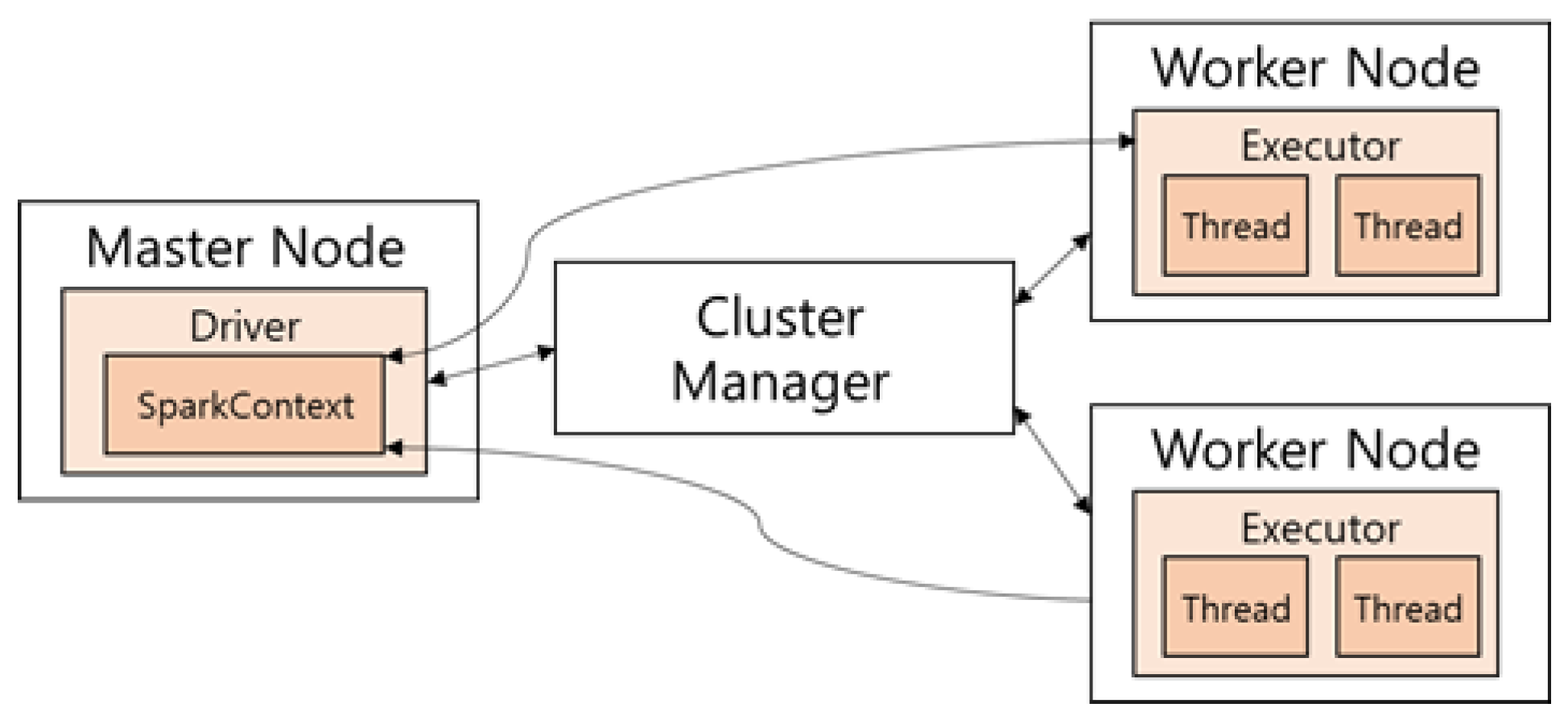
Figure 1. Architecture of Spark.
Symmetry 13 00697 g001
Figure 2. Processing procedure for an RDD.
Symmetry 13 00697 g002
Figure 3. Runtime memory of an executor when processing a transformation map with sufficient memory.
Symmetry 13 00697 g003
Figure 4. Runtime memory of an executor when processing a transformation map with insufficient memory.
Symmetry 13 00697 g004
Figure 5. Process for applying all transformations to elements.
Symmetry 13 00697 g005
Figure 6. Maximum Unrecoverable Memory (MB) of wordcount, k-means clustering, logistic regression, and neural network when the size of element grows.
Symmetry 13 00697 g006
Figure 7. Maximum Unrecoverable Memory (MB) of wordcount, k-means clustering, logistic regression, and neural network when the number of elements per partition grows.
Symmetry 13 00697 g007
Figure 8. Maximum Unrecoverable Memory (MB) of wordcount, k-means clustering, logistic regression, and neural network when the number of partitions grows.
Symmetry 13 00697 g008
Figure 9. Flow diagram of predicting efficient memory size.
Symmetry 13 00697 g009
Figure 10. Prediction accuracy for Element size set1 and Element size set2 of wordcount, k-means clustering, logistic regression, neural network, and CNN when Lasso is used as the machine learning method.
Symmetry 13 00697 g010
Figure 11. Prediction accuracy for Element size set1 and Element size set2 of wordcount, k-means clustering, logistic regression, neural network, and CNN when Ridge is used as the machine learning method.
Symmetry 13 00697 g011
Figure 12. Prediction accuracy for Element size set1 and Element size set2 of wordcount, k-means clustering, logistic regression, neural network, and CNN when RF is used as the machine learning method.
Symmetry 13 00697 g012
Figure 13. Prediction accuracy for Element size set1 and Element size set2 of wordcount, k-means clustering, logistic regression, neural network, and CNN when MLP is used as the machine learning method.
Symmetry 13 00697 g013
Figure 14. Average prediction cost when Lasso and Ridge are applied to wordcount, k-means clustering, logistic regression, neural network, and CNN when input data grow.
Symmetry 13 00697 g014
Figure 15. Prediction cost when RF is applied to wordcount, k-means clustering, logistic regression, neural network, and CNN when input data grow.
Symmetry 13 00697 g015
Figure 16. Prediction cost when MLP is applied to wordcount, k-means clustering, logistic regression, neural network, and CNN when input data grow.
Symmetry 13 00697 g016
Figure 17. Efficiency of wordcount, k-means clustering, logistic regression, neural network, and CNN according to (3) and (4).
Symmetry 13 00697 g017
Table 1. (a) When memory deficiency occurred, actual processing times relative to the shortest possible processing time as memory size increases. (b) When memory oversupply occurred, actual processing times relative to the shortest possible processing time as memory size increases.
(a)
workload\memsize1 GB1.1 GB1.2 GB1.3 GB1.4 GB1.5 GB1.6 GB1.7 GB1.8 GB1.9 GB
wordcountOOMEOOMEOOMEOOMEOOMEOOME1010.70%659.10%238.70%100%
K-MeansOOMEOOMEOOMEOOMEOOMEOOME1123.40%791.00%325.20%100%
logistic regressionOOMEOOMEOOMEOOME1338.70%832.10%583.90%343.80%172.90%100%
neural networkOOMEOOMEOOMEOOMEOOME1265.20%884.50%522.60%281.90%100%
(b)
workload\memsize2 GB3 GB4 GB5 GB6 GB7 GB8 GB9 GB10 GB11 GB
Wordcount100%101.70%101.00%102.40%100.70%100.90%101.60%101.10%100.70%101.70%
K-Means100.20%100%100.50%102.80%100.90%101.60%100.40%101.00%100.20%102.50%
logistic regression100.30%102.90%101.40%100%100.70%101.10%100.90%100.80%102.00%101.40%
neural network103%102.80%103%101.20%101.80%100%100.50%102.70%101.40%100.70%
CNNOOMEOOMEOOMEOOMEOOMEOOME101.90%100.70%100%101.20%
Table 2. Notations for applying series of Spark data-parallel operations to a workload.
NotationDescription
t i i-th Transformation among series of transformation which is applied to partition(s).
P a r t i t i o n i j (i.e., P i j )i-th partition in a RDD that j-th transformation has been applied. If j is 0, no transformation has been applied to the partition.
E l e m e n t i t j (i.e., E i t j )i-th element in a partition that j-th transformation has been applied. If j is 0, no transformation has been applied to the element.
hasnext()A function that checks whether there is the next element.
next()A function that point the next element.
Table 3. Hyperparameters of Lasso and Ridge regression.
Lasso and Ridge
HyperparameterValues
Penalty alpha1 × 10−10, 1 × 10⁻⁵, 0.1, 1, 5, 10, 20
Table 4. Hyperparameters of Random Forest.
RF
Hyper-ParameterValues
# of estimators50, 100, 150
Max featuresauto, sqrt, log2
Max depth50, 100, 150
Table 5. Hyper-parameters of Multi-Layer Perceptron.
Lasso and Ridge
HyperparameterValues
SolverLbfgs, adam, sgd
Activation functionsSigmoid, ReLU
Max iteration1000, 5000, 10,000
Learning rate alpha0.01, 0.05
Hidden layer size50, 100, 150
Table 6. Workload input data description for all workload.
WorkloadElement FormatElement Size
wordcountSet of randomly chosen characters that fulfill element size
(e.g., if element size is 4byte, “abcd”)
Element size set1 = {1 KB, 150 KB, 300 KB, 450 KB, 600 KB, 750 KB, 1 MB}
Element size set2 = {1 KB, 100 KB, 200 KB, 300 KB, 500 KB, 600 KB, 700 KB, 800 KB, 900 KB}
k-means clusteringSet of randomly chosen double type numbers that fulfill element size
(e.g., if element size is 32byte, (1,2,3,4))
logistic regression
neural network
CNNimageOpen image dataset [42]
Publisher’s Note: MDPI stays neutral with regard to jurisdictional claims in published maps and institutional affiliations.