Abstract
Under pure quantum evolution, for a wave packet that diffuses (like a Gaussian), scattering can cause localization. Other forms of the wave function, spreading more rapidly than a Gaussian, are unlikely to localize.
What is the size and shape of a wave packet? I am talking about a wave packet of a particle (atom or molecule) in a gas. Is it a plane wave that fills the container? Or is it a microscopic (perhaps nm) object? I am not talking about a situation where there is a potential holding the particle in some region, like a hydrogen atom. The only things around are other particles, the same or different. (Please see Appendix A). Strangely, this subject has not attracted a lot of attention.
Our conclusion considers a number of possibilities. Should the eventual wave functions be Gaussian or Gaussian-like (to be later defined) then, yes, there is localization. If not, probably no. However, we give an argument that the wave function most likely does become Gaussian. (Generally speaking, people use Gaussians in descriptions, but this is not always warranted).
This paper has three parts: arguments for a Gaussian, localization in that case and the case(s) that it is not a Gaussian. We emphasize that the first part (eventually) treats non-Gaussians that become Gaussian after a number of collisions.
Arguments for a Gaussian. The wave function for a Gaussian would be
In one dimension, a Gaussian in momentum space is
(The following paragraph is the treatment in [1]; for more details, see that reference.) We suppose there is a particle of a different mass and that they scatter. The conservation laws (once they are far enough apart that they do not interact) are
where P and p are collective coordinates: and . In these relations, and () are the momenta and masses of each of the particles, and . Furthermore, we let (). It turns out that, for calculation of the spread, all that matters is the real part of the ( negative) exponent. This changes from , following Equation (3), to
As shown in [1], provided and are significantly different from one another, within a few scattering events the “cross” term in vanishes. This means that the wave functions have ratio of spread such that is constant and there is no cross term—nothing to decohere (and the von Neumann entropy is maximum). In three dimensions the same thing happens, but is more difficult to show [2,3,4]. That, however, is not our main point.
What happens in one dimension if the initial functions are not a Gaussian? We suppose the wave function has the form . This form can fit various other functional forms, e.g., to within 0.06 using 4 coefficients (i.e., elements of the set ). (Please see Appendix B) . Following the earlier method (based on Equation (3)), we find that 4th order terms obey
with () the coefficients of for the respective wave functions. In general, if the deviation from a Gaussian begins with a term there is a matrix that takes one from the values of the coefficients multiplying these terms from before scattering to after scattering. That matrix is
The eigenvalues of this matrix are (for all ) below 1 for and ().
What happens if there is no other-mass particle? I do not know. I would not have thought it should make a difference, but I do not have a proof. In practice, there is almost always some impurity, but it may scatter rarely.
Thus, there is an indication that in one dimension the wave function approaches a Gaussian. In higher dimension—in particular 3—I do not have definitive results. It is still true [1] that for Gaussians the spread approaches a maximum of von Neumann entropy and (if there are two types of particles, and then) .
For three dimensions, there are many ways that power terms can occur; for one can have anything of the form with , and similarly for , leading to coefficients for the two of them. (Please see Appendix C). Moreover, as discussed in [1], the post-scattering values of and involve a rotation, SO(3), not just a flip. Thus, (and for ).
I have examined cubic and quartic components of the logarithm of the wave function. All the indicated operations have been carried out, the cross terms involving momenta of and of have been dropped, and a rather complex recursion for the plethora of coefficients evaluated numerically. Sample results are shown in Figure 1 and Figure 2. The “time” represents the number of scattering events, and the ordinate is the sum total of the absolute values of all cubic or quartic coefficients. Remarkably, they all tend to zero.
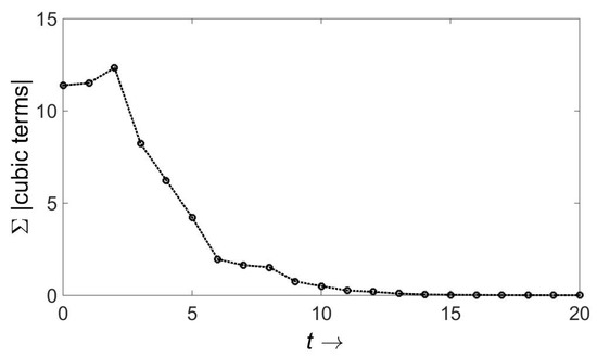
Figure 1.
Reduction of non-Gaussian terms with unequal mass scattering in three dimensions.Because that the problem has an intrinsic nonlinearity, the initial coefficients were varied. Usually they were taken as random between 0 and 1, but on some occasions they were taken to be 20 times that. In all cases there was convergence to zero. The programs to establish this were combinations of symbolic manipulation and numerical evaluation.
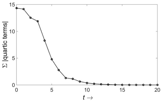
Figure 2.
As in Figure 1, except that this looks at quartic terms. As in the other example, all terms shrink to zero.
Evaluations beyond quartic represent a further problem in symbolic manipulation, but based on the higher-power evidence of one dimension together with the cubic and quartic evidence in three dimensions, it is reasonable to make the claim that all higher power coefficients tend to zero under decoherence.
Is this a proof that eventually everything decoheres to a Gaussian? Absolutely not, but it is an indication.
Localization with Gaussian-like behavior. Scattering can localize. This may be surprising, since some may hold that a wave function can only spread. It turns out (as shown in [2]) that scattering can act like a measurement, that scattering alone can localize. Here we extend that result.
I do not deal with the effects of temperature (cf. [5]), nor with off-diagonal elements of the density matrix [6,7]. I am concerned with pure quantum behavior. Nor do the conclusions depend on interpretation, i.e., they are independent of whether one subscribes to the Copenhagen interpretation (in its many variants), Many Worlds, or some other theory.
I will briefly review the results of [2] and then turn to the extension. (There is a slight change in notation: instead of , we use for convenience in matching results.) The principal consequence of [2] is that, assuming the wave function is a Gaussian, particles do not spread indefinitely. The proof in [2] is a self-consistency argument. We assume two normalized Gaussians in 3 dimensions of the form
with parameters , , and . We assume , so that at time they scatter. Assuming no interaction, at time t this becomes
using center of mass coordinates, the exponent is
where , , and correspondingly for and . Now set (or just afterward). They scatter, but nothing happens to . In the center of mass, we use the Born approximation. Up to normalization, the new wave function is , where we also assumed the interaction was brief, taking place during a short time . With a further condition that , for convenience in integrating, we obtain
(Normalization cancels and can be ignored.) Using this wave function, one can calculate the spread in (), in () and from them and . The latter quantities are then set equal to the original and (both equal to ). Using as the time between collisions (and mass values) we find that indeed the original can be set equal to the final values of spread. To make equations simpler, we define
where ℓ is the scattering length and v a typical velocity. For any given gas, the range of is fixed.
The essential steps in the foregoing derivation are the estimation of , and . It is these that can be generalized.
The first step is to formalize V. Instead of an exponential of range a, we take a potential that is cut off at distance a. This restricts the location of to be within a distance a of . In other words, . This is an additional assumption and may require a larger “a” than was previously posited.
The expectation of is simply , since it is unaffected by the interaction/scattering.
The spread in is another matter and is the principal source of uncertainty in our calculation. For a Gaussian-like initial wave function, we can give estimates. From our previous work [1], we have
Now we would like to weaken the assumptions. It turns out that the most important property (for our purposes) of the Gaussian is its diffusive behavior. This assumption about the spread in the center of mass coordinate is weakened in a specific way: in place of the 8 that appears in the denominator, we allow smaller values, . (In this sense, the wave function is Gaussian-like.) Specifically, and
We now use to arrive at the denominators for the new wave functions of and :
Setting the old equal to the new one, we arrive at a self-consistency criterion for the spread
This is a quadratic equation whose solution is
Taking nm, m/s, nm and gm gm and gives a value of nm, much less than the mean free path. (Please see Appendix D). These are typical parameters for the air and the wave function is localized. Note though that (for air) there is overlap: (number density)Å. Therefore, although the wave functions occupy common volumes, they mostly do not interact.
Not a Gaussian. The essential feature of non-Gaussian wave functions is that the spread in grows. I have not examined the “boundary,” that is, the form of, or parameters in, wave functions that eventually become Gaussian and those that do not. I will though examine various wave functions that are non-Gaussian. Consider, for example, an exponential
We assume that both scattering particles have this form, with the same value of . The spread in the relative coordinate is still bounded by a (or ) but the center of mass coordinate grows. The spread for each, before collision, is . The center of mass coordinate for equal mass particles is , so that the spread for of the center of mass coordinate is also . As a result, the center of mass can also be taken of the form Equation (17). Now apply the free propagator numerically and fit the result to an exponential. Except for particular values of the value of the spread has increased. This means there can be no self-consistent solution (as there was for a Gaussian).
The same happens for the wave function taken as a power.
Conclusions. The point of this is not that no wave function spreads. Rather, it places bounds on spreading for certain wave functions and makes it plausible that scattering is sometimes like a measurement, pinning a particle to a small, localized region.
Funding
This research received no external funding.
Institutional Review Board Statement
Not applicable.
Informed Consent Statement
Not applicable.
Data Availability Statement
Not applicable.
Conflicts of Interest
The authors declare no conflict of interest.
Appendix A
In particular, we do not deal with chains of oscillators or single oscillators, which according to [8,9] (and other literature) become, by decoherence, coherent states, i.e., Gaussian.
Appendix B
The function is not symmetric about ; hence, it requires odd terms in the expansion . This is accomplished with coefficients and that are or less. The fourth order term is about 1/100 of the quadratic term (which is about 1.46).
Appendix C
This is the number of possibilities for both particles and is calculated by imagining the interval as having partitions at 2 (integer) locations (and multiplying by 2). Just to be clear, the 3-dimensional tendency to have a Gaussian wave function is new material.
Appendix D
The minus sign in Equation (16) is spurious and gives an imaginary value for .
References
- Schulman, L.S. Evolution of wave-packet spread under sequential scattering of particles of unequal mass. Phys. Rev. Lett. 2004, 92, 210404. [Google Scholar] [CrossRef] [PubMed]
- Gaveau, B.; Schulman, L.S. Reconciling Kinetic and Quantum Theory. Found. Phys. 2020, 50, 55–60. [Google Scholar] [CrossRef]
- Schulman, L.S.; Schulman, L.J. Convergence of matrices under random conjugation: Wave packet scattering without kinematic entanglement. J. Phys. A 2006, 39, 1717–1728. [Google Scholar] [CrossRef][Green Version]
- Schulman, L.S.; Schulman, L.J. Wave packet scattering without kinematic entanglement: Convergence of expectation values. IEEE Trans. Nanotech. 2004, 4, 8–13. [Google Scholar] [CrossRef]
- Ford, G.W.; O’Connell, R.F. Wave packet spreading: Temperature and squeezing ef- fects with applications to quantum measurement and decoherence. Am. J. Phys. 2002, 70, 319–324. [Google Scholar] [CrossRef]
- Joos, E.; Zeh, H. The Emergence of Classical Properties Through Interaction with the Environment. Z. Phys. B 1985, 59, 223–243. [Google Scholar] [CrossRef]
- Gaveau, B.; Schulman, L.S. Decoherence, the Density Matrix, the Thermal State and the Classical World. J. Stat. Phys. 2017, 169, 889–901. [Google Scholar] [CrossRef]
- Tegmark, M.; Shapiro, H.S. Decoherence produces coherent states: An explicit proof for harmonic chains. Phys. Rev. E 1994, 50, 2538–2547. [Google Scholar] [CrossRef] [PubMed]
- Zurek, W.H.; Habib, S.; Paz, J.P. Coherent States via Decoherence. Phys. Rev. Lett. 1993, 70, 1187–1190. [Google Scholar] [CrossRef] [PubMed]


Publisher’s Note: MDPI stays neutral with regard to jurisdictional claims in published maps and institutional affiliations. |
© 2021 by the author. Licensee MDPI, Basel, Switzerland. This article is an open access article distributed under the terms and conditions of the Creative Commons Attribution (CC BY) license (http://creativecommons.org/licenses/by/4.0/).