Article

Asymptotic Stability of Nonlinear Discrete Fractional Pantograph Equations with Non-Local Initial Conditions

by
Jehad Alzabut
1,*,†,‡,
A. George Maria Selvam
2,
Rami A. El-Nabulsi
3,4,5,
Vignesh Dhakshinamoorthy
2 and
Mohammad E. Samei
6
1
Department of Mathematics and General Sciences, Prince Sultan University, Riyadh 11586, Saudi Arabia
2
Department of Mathematics, Sacred Heart College (Autonomous), Tirupattur 635601, Tamil Nadu, India
3
Biomedical Device Innovation Center, Shenzhen Technology University, 3002 Lantian Road, Pingshan District, Shenzhen 518118, China
4
Research Center for Quantum Technology, Faculty of Science, Chiang Mai University, Chiang Mai 50200, Thailand
5
Athens Institute for Education and Research, Mathematics and Physics Divisions, 8 Valaoritou Street, Kolonaki 10671, Athens, Greece
6
Department of Mathematics, Faculty of Basic Science, Bu-Ali Sina University, Hamedan 65178, Iran
*
Author to whom correspondence should be addressed.
Current address: Department of Mathematics and General Sciences, Prince Sultan University, Riyadh 11586, Saudi Arabia.
These authors contributed equally to this work.
Symmetry 2021, 13(3), 473; https://doi.org/10.3390/sym13030473
Submission received: 22 January 2021 / Revised: 7 March 2021 / Accepted: 8 March 2021 / Published: 13 March 2021

Abstract

:
Pantograph, the technological successor of trolley poles, is an overhead current collector of electric bus, electric trains, and trams. In this work, we consider the discrete fractional pantograph equation of the form Δ β [ k ] ( t ) = w t + β , k ( t + β ) , k ( λ ( t + β ) ) , with condition k ( 0 ) = p [ k ] for t N 1 β , 0 < β 1 , λ ( 0 , 1 ) and investigate the properties of asymptotic stability of solutions. We will prove the main results by the aid of Krasnoselskii’s and generalized Banach fixed point theorems. Examples involving algorithms and illustrated graphs are presented to demonstrate the validity of our theoretical findings.

1. Introduction

Graphical methods in engineering are very much useful to present clear results, develop reasoning, and spatial thinking. Dependency on computer-based simulations has led to the demise of graphical methods [1]. Though computer simulations with the correct programming convey invariably accurate results, they fail to provide ingenuity, understanding, and conceptual thinking. Graphical methods provide practical knowledge which is more efficient than just going through texts. The science of the mechanisms can be extended beyond its classical limits to include pneumatic, hydraulic, electrical, and electronic links.
A special type of differential equation with delay was discovered when J.R. Ockendon and A.B. Tayler studied motion of pantograph head on an electric locomotive [2]. The equation is of the form
x ( t ) = a x ( t ) + b x ( λ t )
where x ( t ) represents the motion of the locomotive and a , b are real constants with 0 < λ < 1 . The pantograph is used in locomotion and trams to transfer power from the wire to the traction unit by maintaining electrical contact. They are also used to increase or reduce motion in some definite proportion, as in the indicator rig on an engine where the motion of the crosshead is reduced proportionally to the desired length of the indicator diagram [3]. The pantograph is a four-bar mechanism used to enlarge or reduce drawings for it is evident that similar curves may be traced as well as straight lines. It was originally used in drafting for copying and scale line drawings. Three-dimensional pantograph is used in sculpting to enlarge sculptures by interchanging the positions. Windscreen wipers on pantograph in some vehicles are used to allow blade to cover more windscreen on each wipe. In 1890, the US census made use of keyboard punch which is a pantograph design [4]. Some heavy-duty applications of pantograph include scissor lifts, material handling equipment, stage lifts, etc. During the past few decades, there was a gradual development of the modeling of nonlinear phenomena that occurs in various science and engineering fields [5].
Fractional calculus, which is a generalization of classical integer order calculus, has become popular among the scientists and engineers as it renders new dimension and flexibility in dealing with real-world problems [6]. Increasing interest towards this field is due to non-local behavior and ultimate convergence to the integer order systems. Potential of fractional derivatives has already been widely explored by researchers from different parts of the world by studying its applications in a range of problems in biology, physics, electronics (circuit theory), chemistry, etc. Non-standard Lagrangians have wide range of applications in nonlinear differential equations, dynamical systems, etc. [7,8,9,10,11,12,13]. Fractional action-like variational approach is very useful in giving better description of dissipative system. The fractional non-standard Lagrangians have been effective in various areas of physics like astrophysics, cosmology, quantum and classical dynamical systems. Recent works can be seen in [14,15,16,17,18]. Discrete fractional calculus is gaining its importance in recent years. Recently, Atici and Eloe [19,20,21,22], and Miller and Ross [23], have studied discrete delta fractional calculus. The study of stability is a venerable branch in the qualitative theory of differential equations. Asymptotic stability results for fractional difference equations have been developed by Chen et al. [24,25,26] for both Caputo- and Riemann Liouville-type operators. Other authors studied stability results of nabla fractional equations [27,28,29]. In 2019, the authors investigated the k-dimensional system of Langevin Hadamard-type fractional differential inclusions with 2 k different fractional orders and they established existence results for a fraction hybrid differential inclusion with Caputo–Hadamard-type fractional derivative [30,31]. In 2020, Zhou et al. studied a nonlinear non-autonomous model which is composed of two species in a rocky intertidal community and occupy each other by individual organisms, in a rocky intertidal community [32]. One can see some significant applications of fractional differential equations in [33,34,35,36,37,38,39,40,41].
Though a standard pantograph equation is available in literature, the varying design of the pantograph in accordance with its application has inspired us to consider the generalized version of the equation. Motivated by the works in [42,43,44,45,46], we consider the nonlinear discrete fractional pantograph equation
Δ β [ k ] ( t ) = w t + β , k ( t + β ) , k ( λ ( t + β ) ) , k ( 0 ) = p [ k ] ,
for t N 1 β , where 0 < β 1 , 0 < λ < 1 , Δ β is a Caputo like difference operator, k represents the motion of the pantograph, w : E R is continuous with respect to k, and t. Here, E = [ 0 , ) × C × C , N t = t , t + 1 , t + 2 , , and  p : C R is Lipschitz continuous in k where C = C ( [ 0 , ) , C ) . That is, there is a positive constant M ( 0 , 1 ) such that
p [ k ] ( t ) p [ l ] ( t ) M k ( t ) l ( t ) ,
for each t N t and almost all k , l C . The discretized form of standard pantograph equation can be obtained from Equation (2) when β = 1 and w t + β , k ( t + β ) , k ( λ ( t + β ) ) = a k ( t + β ) + b k ( λ ( t + β ) ) for t N 1 β . By employing fixed point hypotheses based on Krasnoselskii’s and generalized Banach fixed point theorems, we investigate the asymptotic stability of solutions of Equation (2). Particular examples are presented to demonstrate the validity of our theoretical findings. Some interesting observations are presented at the end of the paper.
This paper is organized as follows. In Section 2, some notations, definitions, and lemmas that are essential in our further analysis are presented. In Section 3, we analyze the asymptotic stability of the problem expressed by (2). Section 4 contains some illustrative examples to show the validity and applicability of our results.

2. Essential Preliminaries

This section is committed to state some notations and essential preliminaries that are acting as necessary prerequisites for the subsequent sections. First, we recall σ th fractional sum of function k C .
Definition 1
([19,20]). Let σ > 0 . The  σ th fractional sum of k is defined by
Δ σ [ k ] ( t ) = 1 Γ ( σ ) s = a t σ ( t s 1 ) ( σ 1 ) k ( s ) ,
where k ( s ) and Δ σ [ k ] ( t ) are defined for s a mod ( 1 ) , for  t ( a + σ ) mod ( 1 ) , respectively,
t ( σ ) = Γ ( t + 1 ) Γ ( t + σ + 1 ) ,
for t N a and Δ σ maps functions defined on N a to functions defined on N a + σ , which, upon substitution in Equation (4), leads to
Δ σ [ k ] ( t ) = 1 Γ ( σ ) s = a t σ Γ ( t s ) Γ ( t s σ + 1 ) k ( s ) .
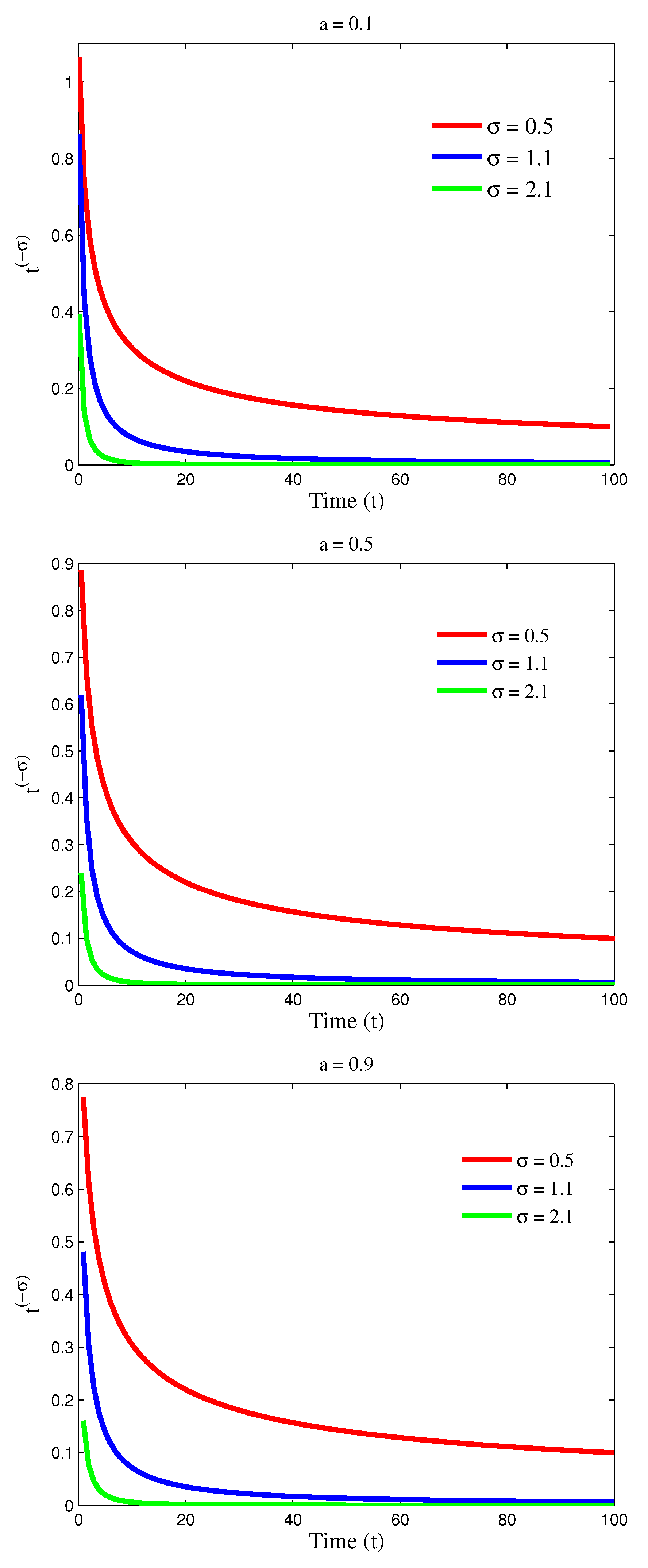
Figure 1 presents the convergence of t ( σ ) in 3-dimensional view, and it is clear that the greater the value of σ , the lesser the time taken for t ( σ ) to approach zero. Figure 2, indeed, illustrates the behavior of t ( σ ) in (5) whenever a and σ are changed, respectively. These results are presented in Table 1, and they show that the operator t ( σ ) is decreasing with respect to both σ and t. Thus, t ( σ ) 0 as t .
Further, the authors of [20] proved that
Δ μ t ( σ ) = Γ ( σ + 1 ) Γ ( σ + μ + 1 ) t ( σ + μ ) ,
for σ R { , 2 , 1 } . At present, suppose that μ > 0 and 1 < μ < , where denotes a positive integer, = μ , here . denotes the ceiling of number [5]. Set σ = μ . The  μ th fractional Caputo-like difference is defined as
Δ μ [ k ] ( t ) = Δ σ Δ [ k ] ( t ) = 1 Γ ( σ ) s = a t σ ( t s 1 ) ( σ 1 ) Δ [ k ] ( s ) ,
where Δ is the th order forward difference operator and Δ μ maps functions defined on N a to functions defined on N a μ .
Lemma 1
([5]). For μ > 0 , μ is non-integer, = μ , σ = μ , it holds
k ( t ) = m = 0 1 ( t a ) ( m ) m ! Δ m [ k ] ( a ) + 1 Γ ( μ ) s = a + σ t σ ( t s 1 ) ( μ 1 ) Δ μ [ k ] ( s ) ,
where k is defined on N a with a Z + . In particular, when 0 < μ < 1 and a = 0 , we have
k ( t ) = k ( 0 ) + 1 Γ ( μ ) s = 1 μ t μ ( t s 1 ) ( μ 1 ) Δ μ [ k ] ( s ) ,
where k is defined on N 1 and Δ μ is defined on N 1 μ .
Algorithm 1: The MATLAB lines of t ( σ ) where σ = 0.5 , 1.1 , 2.1 in (5) for t N a , a = 0.1 , 0.5 , 0.9 and n = 1 , 2 , , N .
      format long
      sigma = [0.5 1.1 2.1];
      [xsigma ysigma] = size(sigma);
      a = [0.1 0.5 0.9];
      N = 100;
      column = 1;
      for    i = 1:ysigma
              for   j = 1:ya
                       n = 1;
                       t = a(j);
                       while t ≤ N
                               parammatrix(n, column) = n;
                               parammatrix(n, column+1) = t;
                               parammatrix(n, column+2) = round(gamma(t + 1)/gamma(t + 1 + sigma(i)), 6);
                               t = t + 1;
                               n = n + 1;
                       end;
                       column = column + 3;
              end;
      end;
Remark 1.
According to Lemma 1, k in (9) should be defined on N 0 . The sum
s = 1 μ t μ ( t s 1 ) ( μ 1 ) Δ μ [ k ] ( s ) ,
has no sense when t = 0 , then we define k on N 1 .
Lemma 2
([20]). Assume that the following factorial functions are well defined.
(i)
If 0 < ν < 1 , then t ( c ν ) t ( ν ) c .
(ii)
t ( ν + c ) = ( t c ) ( ν ) t ( c ) .
Lemma 3
([47]). The quotient expansion of two Gamma functions at infinity is
Γ ( y + a ) Γ ( y + b ) = y a b 1 + O 1 y , arg ( y + a ) < π , | y | .
Definition 2
([25]). Let k = φ ( t ) be a solution of Equation (2).
(1)
The solution k is said to be stable, whenever for any ϵ > 0 and t 0 R + , there exists δ = δ ( t 0 , ϵ ) > 0 such that
k ( t , k 0 , t 0 ) φ ( t ) < ϵ ,
for k 0 φ ( t 0 ) δ ( t 0 , ϵ ) and each t t 0 .
(2)
The solution k is said to be attractive, if there exists η ( t 0 ) > 0 such that k 0 η implies lim t k ( t , k 0 , t 0 ) = 0 .
(3)
The solution k is said to be asymptotically stable, whenever it is stable and attractive.
Definition 3
([48]). Let k = φ ( t ) be a solution of Equation (2). A set Ψ of sequences in l n 0 is uniformly Cauchy or equi-Cauchy, if for every ϵ > 0 , there exists an integer N such that k ( i ) k ( j ) < ϵ whenever i , j > N for every k = k ( n ) in Ψ.
Theorem 1
([48] Discrete Arzelà–Ascoli theorem). A bounded, uniformly Cauchy subset Ω of l n 0 is relatively compact.
Theorem 2
([49] Krasnoselskii fixed point theorem). Let Ψ be a nonempty, closed, convex, and bounded subset of the Banach space X and let G : X X and H : Ψ X be two operators such that
(a)
G is a contraction with constant M < 1 .
(b)
H is continuous, G ( Ψ ) resides in a compact subset of X .
(c)
For all l Ψ , if  k = G ( k ) + H ( l ) then k Ψ .
Then the operator equation G [ k ] + H [ k ] = k has a solution in Ψ.
Lemma 4
([50] Generalized Banach Fixed Point Theorem). Let Ψ be a nonempty, closed subset of a Banach space ( X , · ) and ρ n 0 for every n N 0 such that n = 0 ρ n converges. Moreover, let the mapping Q : Ψ Ψ satisfy the inequality
Q n [ k ] Q n [ l ] ρ n k l ,
for all n N 1 and any k , l Ψ . Then, Q has a uniquely defined fixed point k . Furthermore, for any k 0 Ψ , the sequence Q n [ k 0 ] n = 1 converges to this fixed point k .

3. Main Results

For the purpose of convenience, we set
W λ β [ k ] ( t ) = w t + β , k ( t + β ) , k ( λ ( t + β ) ) .
Let l 1 be the set of all real sequences k = k ( t ) t = 1 with norm
k = sup t N 1 k ( t ) ,
then l 1 is a Banach space. Define the operators G [ k ] ( t ) = p [ k ] ( t ) and
H [ k ] ( t ) = 1 Γ ( β ) s = 1 β t β ( t s 1 ) ( β 1 ) W λ β [ k ] ( s ) , Q [ k ] ( t ) = p [ k ] ( t ) + 1 Γ ( β ) s = 1 β t β ( t s 1 ) ( β 1 ) W λ β [ k ] ( s ) ,
where p : C R is Lipschitz continuous map and W λ β [ k ] ( s ) is defined in Equation (11). Clearly, Q [ k ] = G [ k ] + H [ k ] . Let k , l l β . Then, we have
G [ k ] ( t ) G [ l ] ( t ) = p [ k ] ( t ) p [ l ] ( t ) M k l .
Thus, the operator G is contraction with M < 1 . Condition (a) of the Lemma 2 holds and k ( t ) is a solution of (2) if it is a fixed point of Q. Now, we proof our key lemmas.
Lemma 5.
The map k : N 1 R is a solution of (2) if and only if k ( t ) is a solution of the fractional Taylor’s difference formula given by
k ( t ) = k ( 0 ) + 1 Γ ( β ) s = 1 β t β ( t s 1 ) ( β 1 ) W λ β [ k ] ( s ) ,
for each t N 1 , where W λ β [ k ] ( s ) is defined in (11).
Proof. 
Suppose that k ( t ) is a solution of (2), we have from (9)
k ( t ) = k ( 0 ) + 1 Γ ( β ) s = 1 β t β ( t s 1 ) ( β 1 ) Δ β [ k ] ( s ) = k ( 0 ) + 1 Γ ( β ) s = 1 β t β ( t s 1 ) ( β 1 ) W λ β [ k ] ( s ) .
This implies that (13) holds. Conversely, if  k ( t ) is solution of (13), comparing (9) and (13) yields,
s = 1 β t β ( t s 1 ) ( β 1 ) Δ β [ k ] ( s ) = s = 1 β t β ( t s 1 ) ( β 1 ) W λ β [ k ] ( s ) ,
which takes the form
s = 1 β t β ( t s 1 ) ( β 1 ) Δ β [ k ] ( s ) W λ β [ k ] ( s ) = 0 ,
for each t N 1 . If  t = 1 then (14) becomes
( β 1 ) ( β 1 ) Δ β [ k ] ( 1 β ) W λ β [ k ] ( 1 β ) = 0 ,
which implies
Δ β [ k ] ( 1 β ) = W λ β [ k ] ( 1 β ) .
If t = 2 then from (14) it follows that
( β ) ( β 1 ) Δ β [ k ] ( 1 β ) W λ β [ k ] ( 1 β ) + ( β 1 ) ( β 1 ) Δ β [ k ] ( 2 β ) W λ β [ k ] ( 2 β ) = 0 .
By using (15), the above equation becomes
Δ β [ k ] ( 2 β ) = W λ β [ k ] ( 2 β ) .
Thus, by induction, we have that Δ β [ k ] ( t ) = W λ β [ k ] ( t ) for all t N 1 β and so k ( t ) is a solution of (2). This completes the proof.    □
In order to prove the main results, we make the following assumption.
( W 1 )
There exists constants σ 1 ( β , 1 ) and B 1 , B 2 > 0 such that
w t , k ( t ) , k ( λ t ) ( B 1 + B 2 ) t ( σ 1 ) ,
for t N 1 .
Lemma 6.
Assume that (3) and ( W 1 ) hold. Then, H is continuous and H [ Ψ ] is a compact subset of R for t N 1 , where
Ψ = k ( t ) : k ( t ) t ( ξ 1 ) , t N 1 ,
ξ 1 = 1 2 ( β σ 1 ) satisfies
( B 1 + B 2 ) Γ ( 1 σ 1 ) ( 1 M ) Γ ( 1 + β σ 1 ) ( 1 + ξ 1 ) ( ξ 1 ) 1 .
Proof. 
For t N 1 , ξ 1 > 0
t ( ξ 1 ) = Γ ( t + 1 ) Γ ( t + ξ 1 + 1 ) .
Clearly the set Ψ defined in (17) is closed, bounded, and convex subset of R . First, we prove the continuity of the operator H. Using Equations (7) and (12) and the condition ( W 1 ) , we have
H [ k ] ( t ) = 1 Γ ( β ) s = 1 β t β ( t s 1 ) ( β 1 ) W λ β [ k ] ( s ) 1 Γ ( β ) s = 1 β t β ( t s 1 ) ( β 1 ) W λ β [ k ] ( s ) 1 Γ ( β ) s = 1 β t β ( t s 1 ) ( β 1 ) ( B 1 + B 2 ) ( s + β ) ( σ 1 ) = ( B 1 + B 2 ) Δ β ( t + β ) ( σ 1 ) = ( B 1 + B 2 ) Γ ( 1 σ 1 ) Γ ( 1 + β σ 1 ) ( t + β ) ( β σ 1 ) = ( B 1 + B 2 ) Γ ( 1 σ 1 ) Γ ( 1 + β σ 1 ) ( t + β ) ( 2 ξ 1 ) .
For t N 1 , by using Lemma 2 we obtain
H [ k ] ( t ) ( B 1 + B 2 ) Γ ( 1 σ 1 ) Γ ( 1 + β σ 1 ) ( t + β ) ( 2 ξ 1 ) = ( B 1 + B 2 ) Γ ( 1 σ 1 ) Γ ( 1 + β σ 1 ) ( t + β + ξ 1 ) ( ξ 1 ) ( t + β ) ( ξ 1 ) ( B 1 + B 2 ) Γ ( 1 σ 1 ) Γ ( 1 + β σ 1 ) ( 1 + ξ 1 ) ( ξ 1 ) ( t ) ( ξ 1 ) .
Using (18), it is clear that H [ k ] ( t ) t ( ξ 1 ) . Thus, H [ Ψ ] Ψ for t N 1 . Let ϵ > 0 be given. Then, there exists S 1 N 1 , such that t > S 1 implies
( B 1 + B 2 ) Γ ( 1 σ 1 ) Γ ( 1 + β σ 1 ) t ( β σ 1 ) < ϵ 2 .
Consider the sequence k n such that k n k . By the continuity of the function f and Lemma 5 for t 1 , 2 , S 1 , we obtain
H [ k n ] ( t ) H [ k ] ( t ) 1 Γ ( β ) s = 1 β t β ( t s 1 ) ( β 1 ) W λ β [ k n ] ( s ) W λ β [ k ] ( s ) t ( β ) Γ ( β + 1 ) max s 1 β , , S 1 β W λ β [ k n ] ( s ) W λ β [ k ] ( s ) Γ ( β + S 1 ) Γ ( S 1 ) Γ ( β + 1 ) max s 1 β , , S 1 β W λ β [ k n ] ( s ) W λ β [ k ] ( s ) 0 ,
as n , For t N S 1 + 1 ,
H [ k n ] ( t ) H [ k ] ( t ) 1 Γ ( β ) s = 1 β t β ( t s 1 ) ( β 1 ) W λ β [ k n ] ( s ) W λ β [ k ] ( s ) 2 ( B 1 + B 2 ) Γ ( β ) s = 1 β t β ( t s 1 ) ( β 1 ) ( s + β ) ( σ 1 ) 2 ( B 1 + B 2 ) Γ ( 1 σ 1 ) Γ ( 1 + β σ 1 ) ( t ) ( β σ 1 ) < ϵ .
Thus,
H [ k n ] ( t ) H [ k ] ( t ) 0 ,
as n for all t N 1 . Therefore, the operator H is continuous. Let δ 1 , δ 2 N 1 and δ 1 < δ 2 . Then, we get
H [ k ] ( δ 2 ) H [ k ] ( δ 1 ) 1 Γ ( β ) s = 1 β δ 2 β ( δ 2 s 1 ) ( β 1 ) W λ β [ k ] ( s ) + 1 Γ ( β ) s = 1 β δ 1 β ( δ 2 s 1 ) ( β 1 ) W λ β [ k ] ( s ) ( B 1 + B 2 ) Γ ( 1 σ 1 ) Γ ( 1 + β σ 1 ) δ 2 ( β σ 1 ) + ( B 1 + B 2 ) Γ ( 1 σ 1 ) Γ ( 1 + β σ 1 ) δ 1 ( β σ 1 ) < ϵ .
It is clear from the definition of uniformly Cauchy that H [ k ] , k Ψ is bounded and uniformly Cauchy subset and from Discrete Arzelà–Ascoli’s Theorem stated in Lemma 1, H [ Ψ ] is relatively compact. This completes the proof.    □
Lemma 7.
Assume that (3) and condition ( W 1 ) hold, then for t N 1 a solution of (2) is in Ψ.
Proof. 
Condition (c) of Lemma 2 is yet to be proved. If  k = G [ k ] + H [ l ] , l Ψ for t N 1 , we have
k ( t ) G [ k ] ( t ) + H [ l ] ( t ) p [ k ] ( t ) + ( B 1 + B 2 ) Γ ( 1 σ 1 ) Γ ( 1 + β σ 1 ) ( t + β ) ( β σ 1 ) M k ( t ) + ( B 1 + B 2 ) Γ ( 1 σ 1 ) Γ ( 1 + β σ 1 ) ( t + β ) ( β σ 1 ) .
Therefore,
k ( t ) ( B 1 + B 2 ) Γ ( 1 σ 1 ) Γ ( 1 + β σ 1 ) ( 1 M ) ( t ) ( β σ 1 ) ( B 1 + B 2 ) Γ ( 1 σ 1 ) ( 1 M ) Γ ( 1 + β σ 1 ) ( 1 + ξ 1 ) ( ξ 1 ) t ( ξ 1 ) .
Indeed k ( t ) t ( ξ 1 ) . Thus, k ( t ) Ψ for t N 1 . By Theorem 2, Q has a fixed point in Ψ which is solution of (2).    □
Theorem 3.
Assume that (3) and condition ( W 1 ) hold, then the solutions of (2) are attractive.
Proof. 
By Lemma 7, the solutions of (2) exist and are in Ψ . Further, the function k ( t ) in Ψ tends to zero as t . Then, clearly the solutions of (2) tend to zero with t approaching infinity. The proof is complete.    □
Before establishing the theorems, we make the following assumption.
( W 2 )
There exists σ 2 ( β , 1 ) and B 3 , B 4 0 such that
w ( t , k 1 ( t ) , l 1 ( t ) ) w ( t , k 2 ( t ) , l 2 ( t ) ) B 3 k 1 k 2 + B 4 l 1 l 2 t ( σ 2 ) ,
for any k i , l i l , i = 1 , 2 .
Theorem 4.
Assume that (3) together with the condition ( W 2 ) is satisfied, then the solution of (2) is unique bounded solution in l provided that
ρ = M + ( B 3 + B 4 ) Γ ( 1 σ 2 ) Γ ( 1 + β σ 2 ) Γ ( 2 β + σ 2 ) < 1 .
Proof. 
Let the iterates of operator Q be defined as Q 1 = Q and Q n = Q ( Q n 1 ) for each n N 1 . Now, we shall prove that Q is a contraction operator for sufficiently large n. We have that
Q n [ k ] Q n [ l ] ρ n k l
and
Q [ k ] ( t ) Q [ l ] ( t ) p [ k ] p [ l ] + 1 Γ ( β ) s = 1 β t β ( t s 1 ) ( β 1 ) W λ β [ k n ] ( s ) W λ β [ k ] ( s ) M k l + ( B 3 + B 4 ) Γ ( 1 σ 2 ) Γ ( 1 + β σ 2 ) ( t ) ( β σ 2 ) k l M k l + ( B 3 + B 4 ) Γ ( 1 σ 2 ) Γ ( 1 + β σ 2 ) ( 1 ) ( β σ 2 ) k l M + ( B 3 + B 4 ) Γ ( 1 σ 2 ) Γ ( 1 + β σ 2 ) Γ ( 2 β + σ 2 ) k l ,
which implies
Q [ k ] Q [ l ] ρ k l .
Therefore, the (23) is true for n = 1 . Assuming (23) is true for n, we obtain
Q n + 1 [ k ] ( t ) Q n + 1 [ l ] ( t ) = Q ( Q n ) [ k ] Q ( Q n ) [ l ] p [ Q n [ k ] ] p [ Q n [ l ] ] + 1 Γ ( β ) s = 1 β t β ( t s 1 ) ( β 1 ) W λ β [ Q n [ k ] ] ( s ) W λ β [ Q n [ l ] ] ( s ) ρ n M k l + ( B 3 + B 4 ) ρ n Γ ( 1 σ 2 ) Γ ( 1 + β σ 2 ) ( t ) ( β σ 2 ) k l M k l + ( B 3 + B 4 ) Γ ( 1 σ 2 ) Γ ( 1 + β σ 2 ) ( 1 ) ( β σ 2 ) k l ρ n M + ( B 3 + B 4 ) Γ ( 1 σ 2 ) Γ ( 1 + β σ 2 ) Γ ( 2 β + σ 2 ) k l ,
which implies
Q n + 1 [ k ] Q n + 1 [ l ] ρ n + 1 k l .
By the principle of mathematical induction on n, the statement (23) is true for all n N 1 . The geometric series n = 0 ρ n converges, as  ρ < 1 and so Q has a unique bounded fixed point in Ψ .    □
Theorem 5.
Assume that (3) and condition ( W 2 ) hold, then the solutions of (2) are stable provided that (22) holds.
The proof follows from Theorem 4.
Theorem 6.
Assume that (3) and conditions ( W 1 ) and ( W 2 ) hold. Then, the solutions of (2) are asymptotically stable provided that (22) holds.
The proof is the consequence of Theorems 3 and 5.

4. Numerical Examples

Example 1.
Consider the following discrete fractional pantograph equation,
Δ 0.8 [ k ] ( t ) = 1 10 0.04 k ( t + 0.8 ) + 0.01 sin k t + 0.8 2 , k ( 0 ) = p [ k ] ,
for each t N 0.2 , where
p [ k ] 0.2 k .
Clearly, β = 0.8 ( 0 , 1 ] , M = 0.2 ( 0 , 1 ) , λ = 1 2 ( 0 , 1 ) . Take
W λ β [ k ] ( t ) = 1 10 0.04 k ( t + 0.8 ) + 0.01 sin k t + 0.8 2 .
Let k 1 , k 2 , l 1 , l 2 C . Then, we have
w t , k 1 ( t ) , l 1 ( λ t ) w t , k 2 ( t ) , l 2 ( λ t ) = 1 10 0.04 k 1 ( t + 0.8 ) + 0.01 sin l 1 t + 0.8 2 1 10 0.04 k 2 ( t + 0.8 ) + 0.1 sin l 2 t + 0.8 2 0.004 k 1 ( t + 0.8 ) k 2 ( t + 0.8 ) + 0.001 sin l 1 t + 0.8 2 sin l 2 t + 0.8 2 0.004 k 1 ( t + 0.8 ) k 2 ( t + 0.8 ) + 0.001 l 1 t + 0.8 2 l 2 t + 0.8 2 .
Then, from (21), for  σ 2 = 0.85 ( β , 1 ) , we get
w t , k 1 ( t ) , l 1 ( λ t ) w t , k 2 ( t ) , l 2 ( λ t ) 0.004 k 1 ( t + 0.8 ) k 2 ( t + 0.8 ) + 0.001 l 1 ( t + 0.8 ) l 2 ( t + 0.8 ) t ( 0.85 ) ,
for all t N 1 β = N 0.2 = 0.2 , 1.2 , 2.2 , .
By using (5) and consider three sample values for σ, we will have
t ( σ 2 ) = Γ ( t + 1 ) Γ ( t + σ 2 + 1 ) = Γ ( t + 1 ) Γ ( t + 0.81 + 1 ) = 0.9143 , 0.5458 , , 0.1109 , Γ ( t + 1 ) Γ ( t + 0.90 + 1 ) = 0.8774 , 0.5014 , , 0.0866 , Γ ( t + 1 ) Γ ( t + 0.99 + 1 ) = 0.8379 , 0.4591 , , 0.0676 ,
for t = 0.2 , 1.2 , , 14.2 respectively. Table 2 shows these numerical results. Therefore,
B 3 = 0.004 , B 4 = 0.001 .
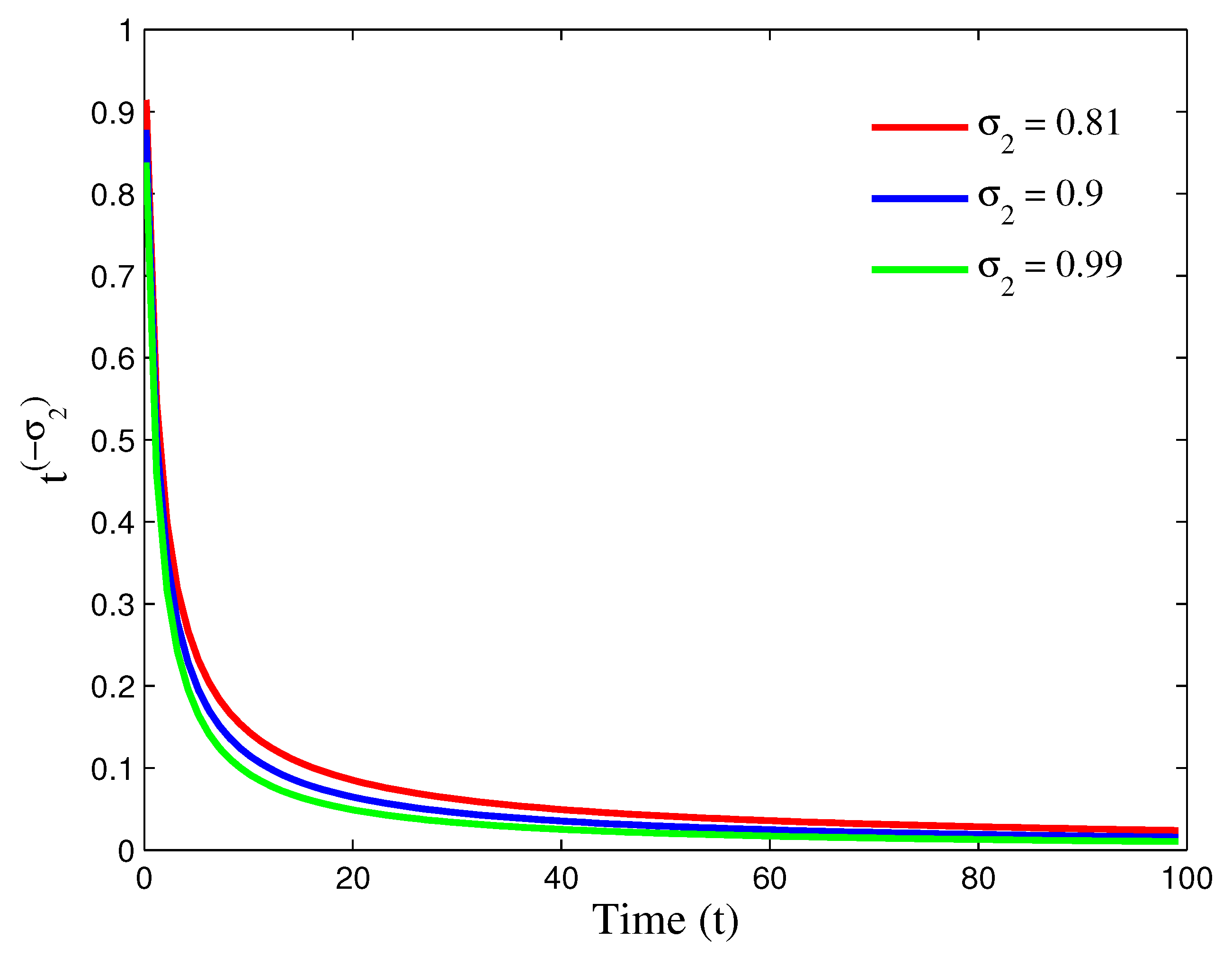
Figure 3 illustrates t ( σ 2 ) for σ 2 = 0.81 , 0.90 , 0.99 and t N 0.2 . These results are shown in Table 2.
Now, by employing Equation (22), the  ρ obtained for different fractional order β and for different values of σ 2 . For this purpose, let σ 2 = 0.81 , 0.90 , and 0.99 , and because σ 2 should be in ( β , 1 ) , then we have
ρ = M + ( B 3 + B 4 ) Γ ( 1 σ 2 ) Γ ( 1 + β σ 2 ) Γ ( 2 β + σ 2 ) = 0.2 + 0.005 Γ ( 1 0.81 ) Γ ( 1 + β 0.81 ) Γ ( 2 β + 0.81 ) , 0.2 + 0.005 Γ ( 1 0.90 ) Γ ( 1 + β 0.90 ) Γ ( 2 β + 0.90 ) , 0.2 + 0.005 Γ ( 1 0.99 ) Γ ( 1 + β 0.99 ) Γ ( 2 β + 0.99 ) , = 0.2 + 0.005 Γ ( 0.19 ) Γ ( β + 0.19 ) Γ ( 2.81 β ) = 0.2030 , 0.2039 , , 0.2240 , 0.2 + 0.005 Γ ( 0.10 ) Γ ( β 0.10 ) Γ ( 2.90 β ) = 0.2027 , 0.2044 , , 0.2451 , 0.2 + 0.005 Γ ( 0.01 ) Γ ( β 0.01 ) Γ ( 2.99 β ) = 0.2025 , 0.2163 , , 0.6768 ,
for
β = 0.05 , 0.10 , 0.15 , , 0.8 ,
whenever σ 2 = 0.81 , for 
β = 0.05 , 0.10 , 0.15 , , 0.9 ,
whenever σ 2 = 0.90 , for 
β = 0.05 , 0.10 , 0.15 , , 0.95 ,
whenever σ 2 = 0.99 , respectively.
The solution is given by
k ( t ) = p ( k ) + 1 Γ ( 0.8 ) s = 0.2 t 0.8 ( t s 1 ) ( β 1 ) × 1 10 0.04 k ( s + 0.8 ) + 0.01 sin k s + 0.8 2 ,
for almost all t N 1 . Simple calculations yield,
B 3 = 0.004 , B 4 = 0.001 ,
M = 0.2 , σ 2 = 0.85 and ρ = 0.2295 . The conditions in Theorem 4 hold and thus the solutions of (24) are asymptotically stable.
Remark 2.
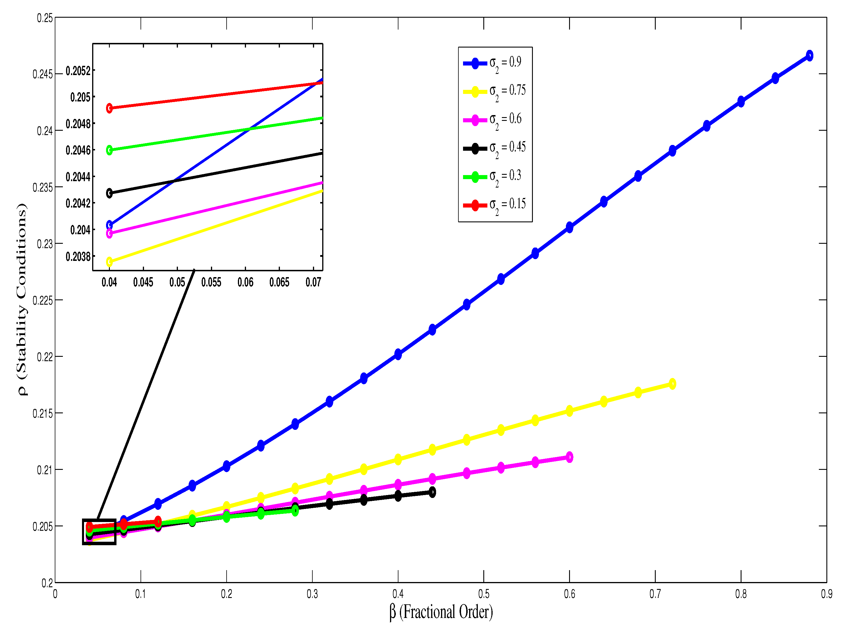
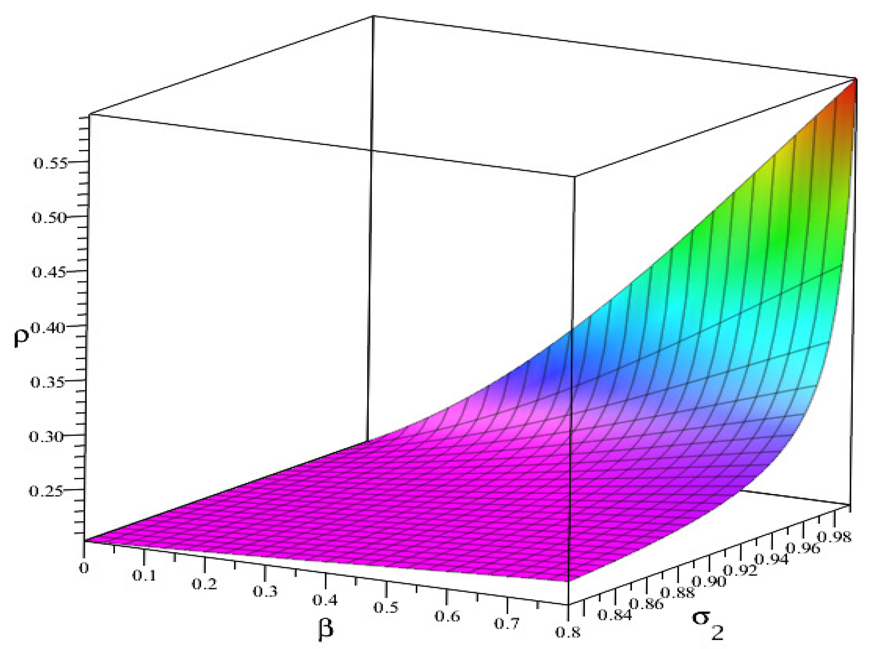
It is clear from Figure 4 that the increase in fractional order ( β ) results in gradual increase in the value of ρ in (22) and all the values of ρ are less than one. The values of ρ are tabulated in Table 3 which ensures the stability of (24). The value of ρ is plotted against β ( 0 , 0.8 ) and σ 2 in the range ( 0.8 , 1 ) in Figure 5. Thus, it is evident that the solutions of discrete fractional equations of order β = 0.8 remains stable ( i . e . , ρ < 1 ) for any values of σ 2 ( 0.8 , 1 ) .
Algorithm 2: The MATLAB lines of t ( σ 2 ) where σ = 0.81 , 0.9 , 0.99 in Example 1 for t N 1 β , t = 0.2 , 1.2 , 2.2 , , 14.2 and n = 1 , 2 , , N .
      format long
      sigma = [0.81 0.9 0.99];
      [xsigma ysigma] = size(sigma);
      beta = 0.2;
      N = 100;
      column = 1;
      for    i = 1:ysigma
               n = 1;
               t = beta;
               while t ≤ N
                               parammatrix(n, column) = n;
                               parammatrix(n, column+1) = t;
                               parammatrix(n, column+2) = round(gamma(t + 1)/gamma(t + 1 + sigma(i)), 6);
                               t = t + 1;
                               n = n + 1;
                       end;
                       column = column + 3;
      end;
Example 2.
Consider the following discrete fractional pantograph equation,
Δ 0.5 [ k ] ( t ) = 1 25 0.09 k ( t + 0.5 ) + 0.3 cos 2 k t + 0.5 5 , k ( 0 ) = p [ k ] ,
for each t N 0.5 , where
p [ k ] 0.1 k .
Clearly, β = 0.5 ( 0 , 1 ] , M = 0.1 ( 0 , 1 ) , λ = 1 5 ( 0 , 1 ) . Take
W λ β [ k ] ( t ) = 1 25 0.09 k ( t + 0.5 ) + 0.3 cos 2 k t + 0.5 5 .
Let k 1 , k 2 , l 1 , l 2 C . Then, we have
w t , k 1 ( t ) , l 1 ( λ t ) w t , k 2 ( t ) , l 2 ( λ t ) = 1 25 0.09 k 1 ( t + 0.5 ) + 0.3 cos 2 l 1 t + 0.5 5 1 25 0.09 k 2 ( t + 0.5 ) + 0.3 cos 2 l 2 t + 0.5 5 9 2500 k 1 ( t + 0.5 ) k 2 ( t + 0.5 ) + 3 250 cos 2 l 1 t + 0.5 5 cos 2 l 2 t + 0.8 5 9 2500 k 1 ( t + 0.5 ) k 2 ( t + 0.5 ) + 3 250 l 1 t + 0.5 5 l 2 t + 0.5 5 .
Then, from (21), for  σ 2 = 0.75 ( β , 1 ) , we get
w t , k 1 ( t ) , l 1 ( λ t ) w t , k 2 ( t ) , l 2 ( λ t ) 0.0036 k 1 ( t + 0.5 ) k 2 ( t + 0.5 ) + 0.012 l 1 ( t + 0.5 ) l 2 ( t + 0.5 ) t ( 0.75 ) ,
for all t N 1 β = N 0.5 = 0.5 , 1.5 , 2.5 , .
By using (5) and consider three sample values for σ, we will have
t ( σ 2 ) = Γ ( t + 1 ) Γ ( t + σ 2 + 1 ) = Γ ( t + 1 ) Γ ( t + 0.55 + 1 ) = 0.8669 , 0.6343 , , 0.2232 , Γ ( t + 1 ) Γ ( t + 0.75 + 1 ) = 0.7821 , 0.5214 , , 0.1287 , Γ ( t + 1 ) Γ ( t + 0.9 + 1 ) = 0.7134 , 0.4459 , , 0.0851 ,
for t = 0.5 , 1.5 , , 14.5 , respectively. Table 4 contains values of t ( σ 2 ) for σ 2 = 0.55 , 0.75 , 0.9 and t N 0.5 . Therefore, B 3 = 0.0036 and B 4 = 0.012 . Now, by employing Equation (22), the  ρ obtained for different fractional order β and for different values of σ 2 . For this purpose, let σ 2 = 0.55 , 0.75 , and 0.9 , and because σ 2 should be in ( β , 1 ) , then we have
ρ = M + ( B 3 + B 4 ) Γ ( 1 σ 2 ) Γ ( 1 + β σ 2 ) Γ ( 2 β + σ 2 ) = 0.1 + 0.0156 Γ ( 1 0.55 ) Γ ( 1 + β 0.55 ) Γ ( 2 β + 0.55 ) , 0.1 + 0.0156 Γ ( 1 0.75 ) Γ ( 1 + β 0.75 ) Γ ( 2 β + 0.75 ) , 0.1 + 0.0156 Γ ( 1 0.9 ) Γ ( 1 + β 0.9 ) Γ ( 2 β + 0.9 ) .
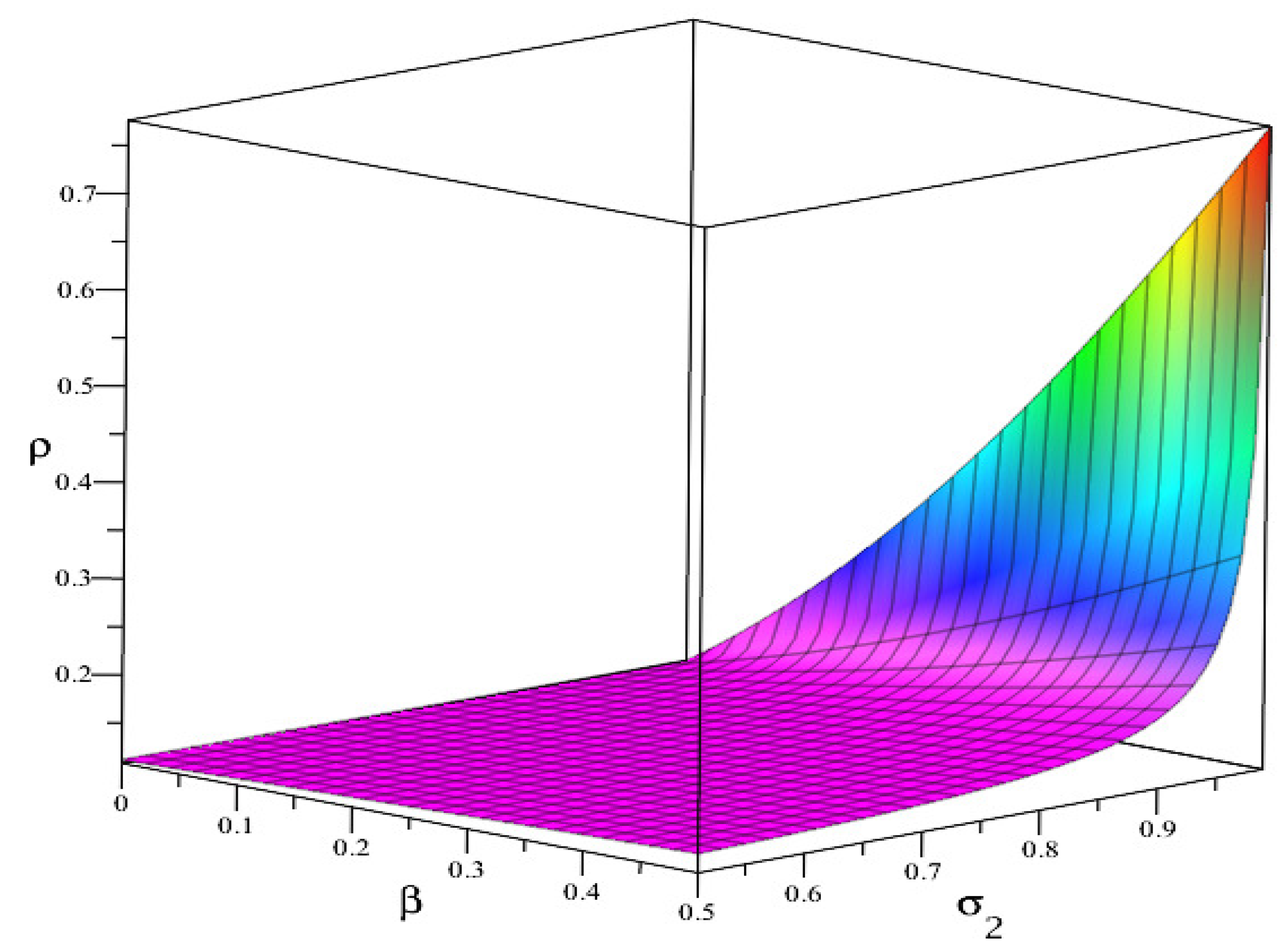
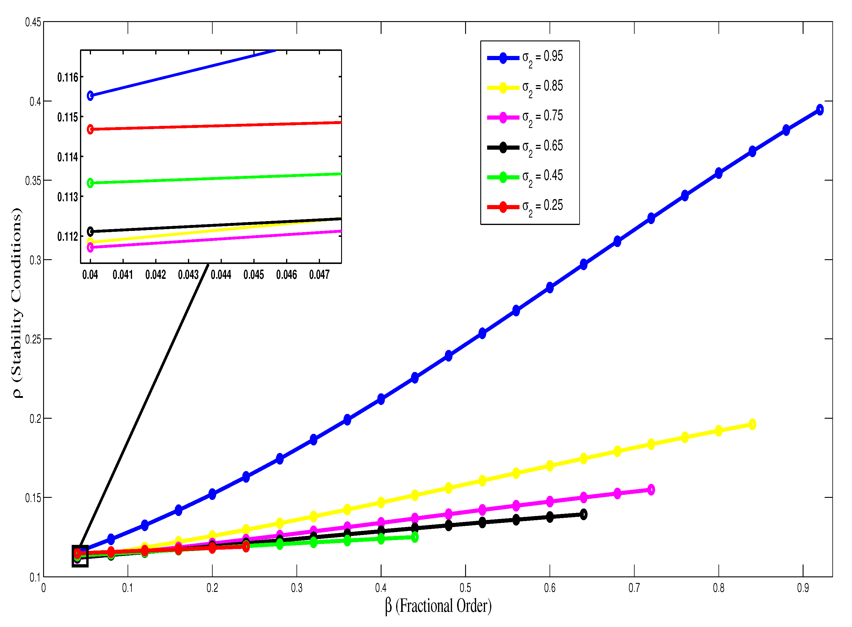
The conditions in Theorem 4 hold and are plotted against the fractional order ( β ) and σ 2 in Figure 6. Figure 7 presents the corresponding 2-dimensional plot of ρ against the fractional order ( β ) for fixed values of σ 2 = { 0.25 , 0.45 , 0.65 , 0.75 , 0.85 , 0.95 } and numerical values are tabulated in Table 5. Thus, the solutions of (26) are asymptotically stable.
Algorithm 3: The MATLAB lines of ρ where σ 2 { 0.15 , 0.30 , 0.45 , 0.60 , 0.75 , 0.9 } for β ( 0 , 1 ) in Example 1.
      format long
      M = 0.2;
      B3 = 0.004; B4 = 0.001;
      beta = 0.04;
      sigma = [0.15 0.3 0.45 0.6 0.75 0.9];
      [xsigma ysigma] = size(sigma);
      n = 1;
      while beta < 1
               column = 1;
               for i = 1:ysigma
                     if sigma(i)>beta
                         parammatrix(n, column) = n;
                         parammatrix(n, column + 1) = beta;
                         parammatrix(n, column + 2) = sigma(i);
                         parammatrix(n, column + 3) = round(M + (B3 + B4) ⋯
                         *gamma(1-sigma(i))/(gamma(1 + beta-sigma(i))⋯
                         *gamma(2-beta + sigma(i))), 6);
                     end;
                     column = column + 4;
               end;
      beta = beta + 0.04;
      n = n + 1;
      end;
Algorithm 4: The MATLAB lines of ρ where β ( 0 , 1 ) where σ 2 = 0.25 , 0.45 , 0.65 , 0.75 , 0.85 , 0.95 in (26).
      format long
      M = 0.1;
      B3 = 0.0036; B4 = 0.012;
      sigma = [0.25 0.45 0.65 0.75 0.85 0.95];
      [xsigma ysigma] = size(sigma);
      for    i = 1:ysigma
               column = 1;;
               beta = 0.04;
               while beta < sigma(i)
                        parammatrix(i, column) = i;
                        parammatrix(i, column + 1) = sigma(i);
                        parammatrix(i, column + 2) = beta;
                        parammatrix(i, column + 3) = round(M + (B3 + B4)⋯
                        *gamma(1-sigma(i))/(gamma(1 + beta-sigma(i))⋯
                        *gamma(2-beta + sigma(i))), 6);
                        beta = beta + 0.04;
                        column = column + 4;
                end;
      end;

5. Conclusions

Asymptotic stability of the initial value discrete fractional pantograph equation is established using Krasnoselskii theorem, generalized Banach fixed point theorem, and discrete Arzelà-Ascoli theorem. Numerical simulations are carried out for the stability results illustrating the effects of the fractional order on the stability conditions. The values are tabulated and plotted. The 3-dimensional images are presented to analyze the stability of the equation with simultaneous variation of the fractional order and σ 2 ( β , 1 ) .

Author Contributions

All authors declare that the study was realized in collaboration with equal responsibility. All authors have read and agreed to the published version of the manuscript.

Funding

J. Alzabut would like to thank Prince Sultan University for funding this work.

Institutional Review Board Statement

Not applicable.

Informed Consent Statement

Not applicable.

Data Availability Statement

Not applicable.

Acknowledgments

J. Alzabut would like to thank Prince Sultan University for supporting this work.

Conflicts of Interest

The authors declare no conflict of interest.

References

  1. Parker, S.P. An Introduction to the Fractional Calculus and Fractional Difference Equations, 2nd ed.; McGraw-Hill Encyclopedia of Engineering Art, Mechanism; McGraw-Hill: New York, NY, USA, 1992; pp. 697–700. [Google Scholar]
  2. Ockendon, J.R.; Tayler, A.B. The dynamics of a current collection system for an electric locomotive. Proc. R. Soc. Lond. Ser. A 1971, 322, 447–468. [Google Scholar]
  3. Schwamb, P.; Merrill, A.L.; James, W.H. Elements of Mechanism, 6th ed.; John Wiley & Sons: New York, NY, USA, 1947. [Google Scholar]
  4. Truesdell, L.E. The Development of Punch Card Tabulation in the Bureau of the Census: 1890–1940; GPO: Washington, DC, USA, 1965. [Google Scholar]
  5. Anastassiou, G.A. Discrete Fractional Calculus and Inequalities. J. Comput. Anal. Appl. 2017, 25, 889–898. [Google Scholar]
  6. Podlubny, I. Fractional Differential Equations; Academic Press: San Diego, CA, USA, 1999. [Google Scholar]
  7. Carinena, J.F.; Ranada, M.F.; Santander, M. Lagrangian formalism for nonlinear second-order Riccati systems: One-dimensional integrability and two-dimensional superintegrability. J. Math. Phys. 2005, 46, 062703. [Google Scholar] [CrossRef] [Green Version]
  8. Carinera, J.F. Non-standard Hamiltonian structures of the Lienard equation and contact geometry. Int. J. Geom. Meth. Mod. Phys. 2019, 16, 1940001. [Google Scholar] [CrossRef]
  9. El-Nabulsi, R.A. Nonlinear dynamics with nonstandard Lagrangians. Qual. Theor. Dyn. Syst. 2012, 12, 273–291. [Google Scholar] [CrossRef]
  10. El-Nabulsi, R.A. Non-standard fractional Lagrangians. Nonlinear Dyn. 2013, 74, 381–394. [Google Scholar] [CrossRef]
  11. El-Nabulsi, R.A. Non-standard power-law Lagrangians in classical and quantum dynamics. Appl. Math. Lett. 2015, 43, 120–127. [Google Scholar] [CrossRef]
  12. El-Nabulsi, R.A. Non-standard Lagrangians in rotational dynamics and the modified Navier-Stokes equation. Nonlinear Dyn. 2015, 79, 2055–2068. [Google Scholar] [CrossRef]
  13. Musielak, Z.E.; Roy, D.; Swift, K.D. Method to derive Lagrangian and Hamiltonian for a nonlinear dynamical system with variable coefficients. Chaos Solitons Fractals 2008, 38, 894–902. [Google Scholar] [CrossRef]
  14. El-Nabulsi, R.A. Fractional oscillators from non-standard Lagrangians and time-dependent fractional exponent. Comp. Appl. Math. 2014, 33, 163–179. [Google Scholar] [CrossRef]
  15. El-Nabulsi, R.A. Fractional variational symmetries of Lagrangians, the fractional Galilean transformation and the modified Schro¨dinger equation. Nonlinear Dyn. 2015, 81, 939–948. [Google Scholar] [CrossRef]
  16. Zhang, Y.; Wang, X.P. Symmetry and invariants of quasi-fractional dynamical systems with non-standard Lagrangians. Symmetry 2019, 11, 1061. [Google Scholar] [CrossRef] [Green Version]
  17. Jiang, J.; Feng, Y.; Xu, S. Noether’s symmetries and its inverse for fractional logarithmic Lagrangian systems. J. Syst. Sci. Inform. 2019, 7, 90–98. [Google Scholar] [CrossRef]
  18. El-Nabulsi, R.A. A fractional approach to nonconservative Lagrangian dynamical systems. Fiz. A 2005, 14, 289–298. [Google Scholar]
  19. Atici, F.M.; Eloe, P.W. Initial Value problems in discrete fractional calculus. Proc. Am. Math. Soc. 2009, 137, 981–989. [Google Scholar] [CrossRef]
  20. Atici, F.M.; Eloe, P.W. A transform method in discrete fractional calculus. Int. J. Differ. Eq. 2007, 25, 165–176. [Google Scholar]
  21. Atici, F.M.; Sengul, S. Modeling with fractional difference equations. J. Math. Anal. Appl. 2010, 137, 1–9. [Google Scholar] [CrossRef] [Green Version]
  22. Atici, F.M.; Eloe, P.W. Discrete fractional calculus with the nabla operator. Electron. J. Qual. Theory Differ. Equ. Special. Ed. I 2009, 3, 1–12. [Google Scholar] [CrossRef]
  23. Miller, K.S.; Ross, B. An Introduction To the Fractional Calculus and Fractional Difference Equations; Wiley: New York, NY, USA, 1993. [Google Scholar]
  24. Chen, F.; Luo, X.; Zhou, Y. Existence results for nonlinear fractional difference equation. Adv. Differ. Eq. 2011, 2011, 12. [Google Scholar] [CrossRef] [Green Version]
  25. Chen, F. Fixed points and asymptotic stability of nonlinear fractional difference equations. Electron. J. Asymptot. Theory Differ. Eq. 2011, 39, 1–18. [Google Scholar] [CrossRef]
  26. Chen, F.; Liu, Z. Asymptotic stability results for nonlinear fractional difference equations. J. Appl. Math. 2012, 2012, 14. [Google Scholar] [CrossRef]
  27. Abdeljawad, T.; Alzabut, J.; Zhou, H. Krasnoselskii existence result for nonlinear delay Caputo q-fractional difference equations with applications to Lotka Volterra competition model. Appl. Math. E Notes 2017, 17, 307–318. [Google Scholar]
  28. Alzabut, J.; Abdeljawad, T.; Baleanu, D. Nonlinear delay fractional difference equations with applications on discrete fractional Lotka - Volterra competition model. J. Comput. Anal. Appl. 2017, 25, 889–898. [Google Scholar]
  29. Mohan, J.J.; Shobanadevi, N.; Deekshitulu, G.V.S.R. Stability of nonlinear nabla fractional difference equations using fixed point theorems. Ital. J. Pure Appl. Math. 2014, 32, 165–184. [Google Scholar]
  30. Samei, M.E.; Hedayati, V.; Ranjbar, G.K. The existence of solution for k-dimensional system of Langevin Hadamard-type fractional differential inclusions with 2k different fractional orders. Medit. J. Math. 2020, 17, 37. [Google Scholar] [CrossRef]
  31. Samei, M.E.; Hedayati, V.; Rezapour, S. Existence results for a fraction hybrid differential inclusion with Caputo-Hadamard type fractional derivative. Adv. Differ. Eq. 2019, 2019, 163. [Google Scholar] [CrossRef]
  32. Zhou, H.; Alzabut, J.; Rezapour, S.; Samei, M.E. Uniform persistence and almost periodic solutions of a non-autonomous patch occupancy model. Adv. Differ. Eq. 2020, 2020, 143. [Google Scholar] [CrossRef] [Green Version]
  33. Iswarya, M.; Raja, R.; Rajchakit, G.; Cao, J.; Alzabut, J.; Huang, C. Existence, uniqueness and exponential stability of periodic solution for discrete-time delayed BAM neural networks based on coincidence degree theory and graph theoretic method. Mathematics 2019, 7, 1055. [Google Scholar] [CrossRef] [Green Version]
  34. Pratap, A.; Raja, R.; Alzabut, J.; Dianavinnarasi, J.; Cao, J.; Rajchakit, G. Finite-time Mittag-Leffler stability of fractional-order quaternion-valued memristive neural networks with impulses. Neural Process Lett. 2020, 51, 1485–1526. [Google Scholar] [CrossRef]
  35. Hedayati, V.; Samei, M.E. Positive solutions of fractional differential equation with two pieces in chain interval and simultaneous Dirichlet boundary conditions. Bound. Val. Prob. 2019, 2019, 141. [Google Scholar] [CrossRef]
  36. Kalvandi, V.; Samei, M.E. New stability results for a sum-type fractional q-integro-differential equation. J. Adv. Math. Stud. 2019, 12, 201–209. [Google Scholar]
  37. Samei, M.E.; Yang, W. Existence of solutions for k-dimensional system of multi-term fractional q-integro-differential equations under anti-periodic boundary conditions via quantum calculus. Math. Meth. Appl. Sci. 2020, 43, 4360–4382. [Google Scholar] [CrossRef]
  38. Li, D.; Sun, W.; Wu, C. A Novel Numerical Approach to Time-Fractional Parabolic Equations with Nonsmooth Solutions. Numer. Math. Theory Methods Appl. 2021, 14, 355–376. [Google Scholar]
  39. Čermák, J.; Kisela, T. Stability properties of two-term fractional differential equations. Nonlinear Dyn. 2015, 80, 1673–1684. [Google Scholar] [CrossRef]
  40. Gorenflo, R.; Mainardi, F. Fractional calculus, integral and differential equations of fractional order. In Fractals and Fractional Calculus in Continuum Mechanics; Carpinteri, A., Mainardi, F., Eds.; CISM Courses and Lecture Notes; Springer: Vienna, Austria, 1997; Volume 378, pp. 223–276. [Google Scholar]
  41. Li, Y.; Chen, Y.Q.; Pudlubny, I. Mittag–Leffler stability of fractional order nonlinear dynamic systems. Automatica 2009, 45, 1965–1969. [Google Scholar] [CrossRef]
  42. Bhalekar, S.; Patade, J. Series solution of the pantograph equation and its properties. Fractal Fract. 2017, 1, 16. [Google Scholar] [CrossRef] [Green Version]
  43. Vivek, D.; Kanagarajan, K.; Harikrishnan, S. Dynamics and Stability Results of Fractional pantograph Equations With Complex Order. J. Appl. Nonlinear Dyn. 2018, 7, 179–187. [Google Scholar] [CrossRef]
  44. Balachandran, K.; Kiruthika, S.; Trujillo, J.J. Existence of solutions of nonlinear fractional pantograph equations. Acta Math. Sci. 2013, 33, 1–9. [Google Scholar] [CrossRef]
  45. Derfel, G.A.; Iserles, A. The pantograph equation in the complex plane. J. Math. Anal. Appl. 1997, 213, 117–132. [Google Scholar] [CrossRef] [Green Version]
  46. Li, D.; Zhang, C. Long time numerical behaviors of fractional pantograph equations. Math. Comput. Simul. 2020, 172, 244–257. [Google Scholar] [CrossRef]
  47. Kilbas, A.A.; Srivastava, H.M.; Trujillo, J.J. Theory and Applications of Fractional Differential Equations; North-Holland Mathematics Studies; Elsevier Science B.V.: Amsterdam, The Netherlands, 2006. [Google Scholar]
  48. Cheng, S.S.; Patula, W.T. An Existence theorem for a nonlinear difference equation. Nonlinear Anal. 1993, 20, 193–203. [Google Scholar] [CrossRef]
  49. Burton, T.A.; Furumochi, T. Krasnoselskii’s fixed point theorem and stability. Nonlinear Anal. Theory, Methods Appl. 2002, 49, 445–454. [Google Scholar] [CrossRef]
  50. Boulares, H.; Ardjouni, A.; Laskri, Y. Existence and uniqueness of solutions for nonlinear fractional nabla difference systems with initial conditions. Fract. Differ. Calc. 2017, 7, 247–263. [Google Scholar] [CrossRef] [Green Version]
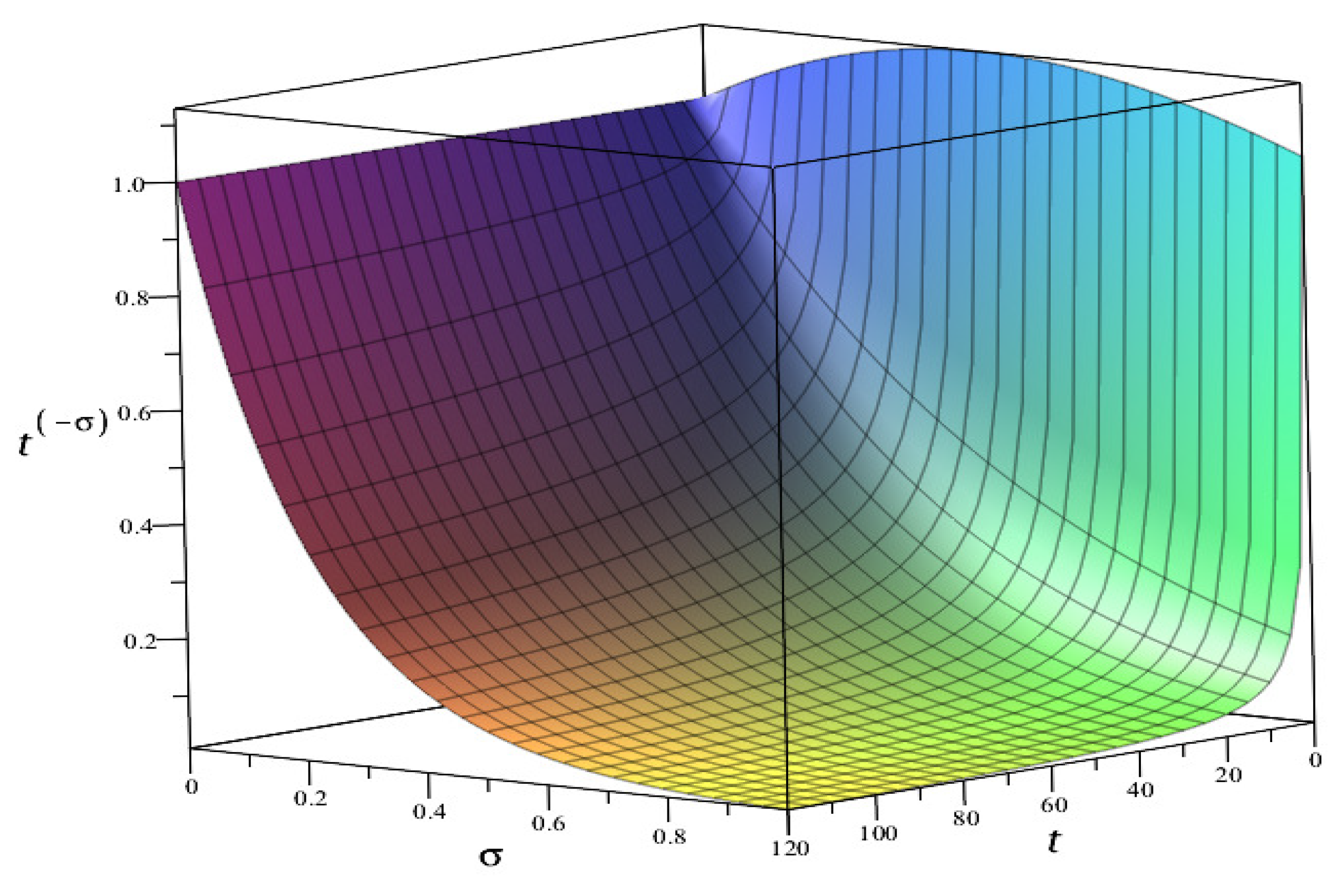
Figure 1. Results of t ( σ ) with respect to t where σ [ 0 , 1 ] in (5).
Symmetry 13 00473 g001
Figure 2. Results of t ( σ ) with respect to t where a = 0.1 , 0.5 , 0.9 in (5) for t N a , σ = 0.5 , 1.1 , 2.1 , respectively, according to Table 1.
Symmetry 13 00473 g002
Figure 3. The behavior of t ( σ 2 ) with respect to t where σ 2 = 0.81 , 0.9 , 0.99 in Example 1, respectively, for t N 0.2 and n = 1 , 2 , , 100 , according to Table 2.
Symmetry 13 00473 g003
Figure 4. ρ versus β where σ 2 { 0.15 , 0.30 , 0.45 , 0.60 , 0.75 , 0.9 } in Example 1, respectively, for β ( 0 , 1 ) , according to Table 3.
Symmetry 13 00473 g004
Figure 5. ρ versus β and σ 2 where β = 0.8 and σ 2 ( 0.8 , 1 ) in Example 1.
Symmetry 13 00473 g005
Figure 6. ρ versus β and σ 2 where β = 0.5 and σ 2 ( 0.5 , 1 ) in Example 2.
Symmetry 13 00473 g006
Figure 7. ρ versus β where σ 2 { 0.25 , 0.45 , 0.65 , 0.75 , 0.85 , 0.95 } in (26), respectively, for β ( 0 , 1 ) , according to Table 5.
Symmetry 13 00473 g007
Table 1. Numerical results of t ( σ ) where σ = 0.5 , 1.1 , 2.1 in (5) for t N a , a = 0.1 , 0.5 , 0.9 and n = 1 , 2 , , 100 (Algorithm 1).
t t ( σ ) t t ( σ ) t t ( σ )
( σ = 0.5 ) n a = 0.1 a = 0.5 a = 0.9
1 0.1 1.06472 0.5 0.88622 0.9 0.77426
2 1.1 0.73200 1.5 0.66467 1.9 0.61295
3 2.1 0.59123 2.5 0.55389 2.9 0.52281
4 3.1 0.50911 3.5 0.48465 3.9 0.46340
5 4.1 0.45377 4.5 0.43618 4.9 0.42049
97 96.1 0.10161 96.5 0.10140 96.9 0.10119
98 97.1 0.10109 97.5 0.10088 97.9 0.10068
99 98.1 0.10057 98.5 0.10037 98.9 0.10017
100 99.1 0.10007 99.5 0.09987 99.9 0.09967
( σ = 1.1 ) n a = 0.1 a = 0.5 a = 0.9
1 0.1 0.86344 0.5 0.61990 0.9 0.48088
2 1.1 0.43172 1.5 0.35763 1.9 0.30455
3 2.1 0.28331 2.5 0.24835 2.9 0.22080
4 3.1 0.20911 3.5 0.18896 3.9 0.17222
5 4.1 0.16488 4.5 0.15184 4.9 0.14065
97 96.1 0.00651 96.5 0.00648 96.9 0.00645
98 97.1 0.00644 97.5 0.00641 97.9 0.00638
99 98.1 0.00636 98.5 0.00634 98.9 0.00631
100 99.1 0.00629 99.5 0.00627 99.9 0.00624
( σ = 2.1 ) n a = 0.1 a = 0.5 a = 0.9
1 0.1 0.392477 0.5 0.238423 0.9 0.160294
2 1.1 0.134913 1.5 0.099343 1.9 0.076139
3 2.1 0.067456 2.5 0.053990 2.9 0.044161
4 3.1 0.040214 3.5 0.033744 3.9 0.028704
5 4.1 0.026593 4.5 0.023007 4.9 0.020093
97 96.1 0.000091 96.5 0.000065 96.9 0.000065
98 97.1 0.000089 97.5 0.000064 97.9 0.000063
99 98.1 0.000087 98.5 0.000063 98.9 0.000062
100 99.1 0.000085 99.5 0.000061 99.9 0.000061
Table 2. Numerical results of  t ( σ 2 ) where σ 2 = 0.81 , 0.90 , 0.99 in Example 1 for t N 1 β = N 0.2 and n = 1 , 2 , , 15 (Algorithm 2).
t ( σ 2 )
n t 0.810.90.99
1 0.2000 0.9143 0.8774 0.8379
2 1.2000 0.5458 0.5014 0.4591
3 2.2000 0.3989 0.3558 0.3166
4 3.2000 0.3184 0.2777 0.2418
5 4.2000 0.2669 0.2287 0.1957
6 5.2000 0.2309 0.1950 0.1644
7 6.2000 0.2042 0.1702 0.1418
8 7.2000 0.1836 0.1513 0.1246
9 8.2000 0.1671 0.1364 0.1112
10 9.2000 0.1536 0.1242 0.1004
11 10.2000 0.1423 0.1141 0.0915
12 11.2000 0.1327 0.1056 0.0841
13 12.2000 0.1244 0.0984 0.0778
14 13.2000 0.1172 0.0921 0.0723
15 14.2000 0.1109 0.0866 0.0676
Table 3. Numerical results of ρ versus σ 2 { 0.15 , 0.30 , 0.45 , 0.60 , 0.75 , 0.9 } for β ( 0 , 1 ) in Example 1 (Algorithm 3).
ρ ( σ 2 )
n β 0.150.300.450.600.750.9
1 0.0400 0.2049 0.2046 0.2043 0.2040 0.2038 0.2040
2 0.0800 0.2052 0.2049 0.2047 0.2045 0.2044 0.2054
3 0.1200 0.2054 0.2052 0.2050 0.2050 0.2052 0.2070
4 0.1600 0.2055 0.2054 0.2055 0.2059 0.2086
5 0.2000 0.2058 0.2058 0.2060 0.2067 0.2103
6 0.2400 0.2061 0.2062 0.2065 0.2075 0.2121
7 0.2800 0.2064 0.2066 0.2071 0.2083 0.2140
8 0.3200 0.2070 0.2076 0.2092 0.2160
9 0.3600 0.2073 0.2081 0.2100 0.2181
10 0.4000 0.2077 0.2086 0.2109 0.2202
11 0.4400 0.2080 0.2092 0.2118 0.2224
12 0.4800 0.2097 0.2126 0.2246
13 0.5200 0.2102 0.2135 0.2268
14 0.5600 0.2106 0.2143 0.2291
15 0.6000 0.2152 0.2314
16 0.6400 0.2160 0.2337
17 0.6800 0.2168 0.2360
18 0.7200 0.2176 0.2382
19 0.7600 0.2404
20 0.8000 0.2425
21 0.8400 0.2446
22 0.8800 0.2466
Table 4. Numerical results of  t ( σ 2 ) where σ 2 = 0.55 , 0.75 , 0.9 in Example 2 for t N 1 β = N 0.5 and n = 1 , 2 , , 15 (Algorithm 2).
t ( σ 2 )
n t 0.550.750.9
1 0.5000 0.8669 0.7821 0.7134
2 1.5000 0.6343 0.5214 0.4459
3 2.5000 0.5199 0.4011 0.3278
4 3.5000 0.4493 0.3303 0.2608
5 4.5000 0.4004 0.2831 0.2173
6 5.5000 0.3640 0.2491 0.1867
7 6.5000 0.3356 0.2233 0.1640
8 7.5000 0.3126 0.2030 0.1464
9 8.5000 0.2936 0.1866 0.1322
10 9.5000 0.2776 0.1729 0.1209
11 10.5000 0.2638 0.1614 0.1114
12 11.5000 0.2517 0.1515 0.1033
13 12.5000 0.2411 0.1429 0.0964
14 13.5000 0.2317 0.1354 0.0903
15 14.5000 0.2232 0.1287 0.0851
Table 5. Numerical results of ρ versus σ 2 { 0.25 , 0.45 , 0.65 , 0.75 , 0.85 , 0.95 } for β ( 0 , 1 ) in (26) (Algorithm 4).
ρ ( σ 2 )
n β 0.250.450.650.750.85
1 0.0400 0.1147 0.1133 0.1121 0.1117 0.1118 0.1155
2 0.0800 0.1156 0.1145 0.1138 0.1138 0.1150 0.1236
3 0.1200 0.1165 0.1157 0.1155 0.1161 0.1183 0.1324
4 0.1600 0.1173 0.1170 0.1173 0.1184 0.1219 0.1419
5 0.2000 0.1181 0.1182 0.1191 0.1209 0.1257 0.1521
6 0.2400 0.1189 0.1194 0.1210 0.1234 0.1296 0.1629
7 0.2800 0.1205 0.1229 0.1259 0.1337 0.1744
8 0.3200 0.1217 0.1248 0.1286 0.1379 0.1864
9 0.3600 0.1228 0.1267 0.1312 0.1423 0.1990
10 0.4000 0.1239 0.1286 0.1339 0.1468 0.2120
11 0.4400 0.1250 0.1305 0.1367 0.1513 0.2255
12 0.4800 0.1324 0.1394 0.1559 0.2393
13 0.5200 0.1342 0.1421 0.1606 0.2534
14 0.5600 0.1360 0.1448 0.1652 0.2678
15 0.6000 0.1377 0.1474 0.1699 0.2823
16 0.6400 0.1393 0.1499 0.1745 0.2969
17 0.6800 0.1524 0.1791 0.3115
18 0.7200 0.1248 0.1835 0.3260
19 0.7600 0.1878 0.3403
20 0.8000 0.1920 0.3544
21 0.8400 0.1961 0.3682
22 0.8800 0.3816
23 0.9200 0.3945
Publisher’s Note: MDPI stays neutral with regard to jurisdictional claims in published maps and institutional affiliations.