1. Introduction
The past several decades have witnessed a gradual increase in the use of robots for assisting humans in various activities from daily housekeeping to military service [
1,
2]. Robot designs have been mostly restricted to a relatively narrow range of stereotypes such as robotic arms, wheeled vehicles, animal-like robots, or humanoids, despite the considerable diversity of tasks for which robots are used. Considering the amount of time and effort required to implement and experiment with novel robot designs, it may be a natural consequence to select a stereotypical design and modify it for a given task. However, considering the large number of possible robot designs, it is highly probable that a more optimal design may exist for a given task; further, this design could be very different from stereotypical designs and may not be discovered via a manual approach.
Recent advances in computational design allow solving non-trivial design problems over a large design space with a reasonable number of computations using various optimization methods in combination with physics-based modeling and simulation of virtual replicas of design solutions. The problem of designing optimal robots with respect to a given task can be addressed computationally by applying an evolutionary algorithm to the population of virtual robots whose motions can be computed precisely in a physics-based simulator. Such a design approach–referred to as evolutionary robot design—has been studied extensively in the robotics and computer graphics communities [
3]. In a typical method for evolutionary robot design, both the body morphology (structure) and the control mechanism (behavior) of each robot are encoded together as a single genotype. The fitness of a robot is evaluated by first converting its genotype to the corresponding phenotype, i.e., the structure and behavior, followed by simulating the robot according to the phenotype, and finally, by measuring how successfully the given task is achieved. Robots with higher fitness have a higher chances of reproduction, which is performed by crossing over the genotypes of selected robots, often with mutations. After generating an initial population of robots randomly, the population is then gradually evolved through successive generations by reproduction and replacement so that the robots in the later generations can have more optimal structures and behaviors than the ones in the earlier generations.
Conventional methods for evolutionary robot design optimize the structure and behavior simultaneously. This simultaneous optimization of both the structure and the behavior, called co-evolution, is at the core of most existing methods in evolutionary robotics and is considered as one of its key strengths, which reflects the close inter-dependency between the mind and the body adequately. In this paper, we present a novel method for the evolutionary robot design. The proposed method differs from the conventional method in that we optimize the structure and behavior alternately instead of simultaneously.
Further, we argue that simultaneous optimization needs to cope with an enormous design space that covers every possible combination of allowable structures and behaviors, which is unnecessarily large and hinders the early discovery of optimal solutions. We considerably reduce the design space by applying an evolutionary algorithm only to the structure and employing a reinforcement learning algorithm for the optimization of the behavior. In contrast to the existing methods that assume both structure and behavior to be innate properties to be inherited, we consider only structure as the innate property. We regard behavior as the learned property, which is not significantly different from biological observations. However, this does not imply a complete separation of the structure and behavior in optimization. As an essential ingredient of our method, we measure the fitness of each structure based on its potential learning ability, which is evaluated by training the robot with the reinforcement learning algorithm and calculating the average of the cumulative episodic rewards of the robot. Thus, our method searches for prospective robotic structures that can potentially lead to near-optimal behaviors if trained sufficiently.
We demonstrate the practical usefulness of our method through experiments based on the virtual replica of an actual modular robot kit, called Tinkerbots [
4]. Given the task of reaching a target location, a large variety of interesting structures and behaviors were designed successfully by our method. In particular, the adaptability of our method was clearly verified by the significant difference between the robots evolved in a clean environment and the robots evolved in a cluttered one.
The remainder of this paper is organized as follows. The previous work closely related to our method is described in
Section 2. The basics of robotic structures and behaviors in our method are introduced in
Section 3. Based on the definitions of structures and behaviors, our key problem to be addressed is formally described in
Section 4. The reinformcent learning algorithm used in our method is explained in
Section 5. The detailed algorithm of our evolutionary method is presented in
Section 6. Several experimental results are displayed and analyzed in
Section 7. The implications of our method are discussed from various viewpoints based on the experimental data in
Section 8. Finally, the key advantages and limitations of our method are summarized in
Section 9.
2. Related Work
The automated design of mechanical structures and robots has been an active research topic in computer graphics through the last decade because of its practical usefulness for computational fabrication [
5]. As an early work in this research area, Zhu and their colleagues introduced a method to synthesize mechanical toys from the user-specified motion of their features based on a parameterized set of mechanical components such as belt pulleys and gears [
6]. A variety of forms, materials, and movement mechanisms were studied afterward for articulated mechanical characters [
7,
8,
9]. However, these methods mainly focused on the design of passive automata mostly moving in place, instead of autonomous robots that could navigate actively. Robots pose an addtional layer of challenges to the problem of automated design because their body structures and their behaviors need to be designed to ensure compatibility and robustness. Megaro et al. presented an interactive method for designing both the structures and motions of 3D-printable robotic creatures, whose capability of stable locomotion could be guaranteed by an optimization process [
10]. More recently, Geilinger et al. developed an optimization-based design method for coping with a broader range of robotic structures with legs and wheels, thereby allowing a flexible array of locomotion styles including walking, rolling, and skating [
11]. In addition, fuzzy systems have been successfully employed in solving non-trivial control problems involved with mechanical structures and nonlinear systems [
12,
13] Our work presents an approach for the computational design of robots; however, we focus on exploring combinatorial design solutions instead of pursuing numerical optimization over a continuous parameter domain.
In robotics, evolutionary approaches such as genetic algorithms have been employed to search for robots over a large design space and to discover the fittest ones through evolution [
3,
14,
15]. Karl Sims demonstrated that a large variety of effective structures and behaviors for artificial creatures, mostly unimaginable in the real world, could be successfully discovered based on genetic algorithms, although their articulated bodies comprised only simple cuboids [
16]. Beyond simulated environments, researchers investigated various approaches for moving artificially evolved creatures to the real world via physical embodiment. Funes and Pollack evolved the design of Lego structures within the range of physically stable ones such that the evolved structures could be built in the real world using tangible Lego bricks [
17]. Lipson and Pollack employed rapid manufacturing technology to minimize human intervention in the process of physical realization of artificial creatures. This technology enabled fabricating robots composed of bars and linear actuators [
18]. Modular architectures have been popularly employed in evolutionary robotics to simplify the implementation of robotic bodies in real hardware, particularly when combined with a focus on evolving a repertoire of representative behaviors including locomotion and self-reconfiguration [
19,
20]. In addition, evolutionary approaches have been effectively utilized for controlling collaborative and competitive behaviors of multiple agents, such as for the teams of robots in robot soccer [
21].
Our work is aligned with these previous studies in that we take an evolutionary approach to the problem of searching for optimal assemblies of modular robots. Similar to how the bodies and brains of animals evolved together, the evolutionary approach is considered reasonable for designing structures and behaviors of robots simultaneously to ensure that they match each other. This has often been referred to as co-evolution or co-optimization [
22]. Lund showed that such a strategy could be executed effectively with real Lego robots through experiments in which both their controllers and morphologies were co-evolved successfully [
23]. Ha et al. presented a method for optimizing the morphological parameters of robots while concurrently adjusting their motion parameters so that the complex relationship between morphology and motion parameters could be established in detail [
24]. Schaff et al. tweaked the traditional reinforcement learning algorithm cleverly to train control policies as well as design distributions by providing the controller access to both the control and design parameters [
25]. In the same vein as these studies, we believe that the structures and behaviors of robots are closely related and need to be designed in a complementary manner. A key difference from the previous methods is that we search for near-optimal structures that can yield near-optimal behaviors by alternating between the evolution of structures and the training of behaviors, instead of optimizing both of those simultaneously. For training behaviors, we use the proximal policy optimization (PPO) algorithm, a popular algorithm among deep reinforcement learning algorithms that has been widely employed in recent robotics research [
26,
27].
3. Structures and Behaviors
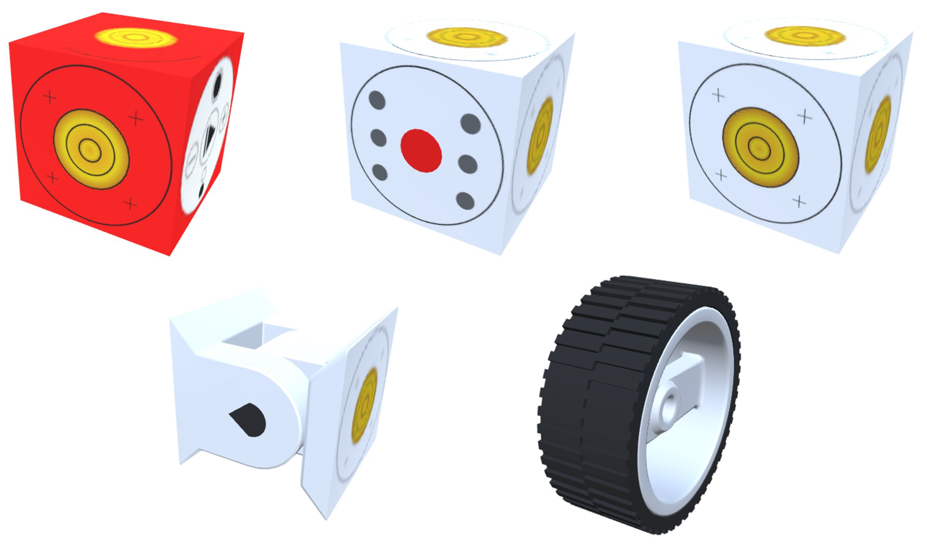
We assume that our robots are constructed in a modular fashion by placing elementary modules together under constraints enforced by each type of module. There are no specific restrictions on the shapes and number of modules and on how the modules are linked to each other as long as the robot can perform the basic functionalities of sensing, computing, and acting through the given modules. For our experiments, we adopted a collection of elementary modules from the Tinkerbots construction kit, as shown in
Figure 1, for its simplicity and flexibility [
4]. The cubical modules are elaborately designed such that any two modules can be easily joined together without additional aids such as cables. The functions and the constraints of each module employed in our implementation are described in detail below.
PowerBrain: A robot must include one and only one PowerBrain module as the central unit of the robot. The physical PowerBrain module in the original kit contains a battery and a simple computer to generate electric power and a control signal. On its front side, a set of input buttons are arranged in a circular layout; thses do not play a significant role in our simulation. Other modules including the motor, pivot, and main modules can be attached to the remaining five sides, where sockets are set up such that both the electric power and control signal from the PowerBrain can be seamlessly transmitted to its attached modules.
Motor: The motor module in the original kit allows two wheels to be fitted into the axles of two opposing motors that are aligned with a pair of opposite sides of the module, such that both wheels can be rotated in a clockwise or counter-clockwise direction simultaneously. In our implementation, we simplified such a connection mechanism between a motor and wheels by removing the existence of axles and axes and by allowing wheels to be connected to the motor directly. Further, we forced the wheels to be attached to a motor in a pairwise manner, thereby excluding the possibility of attaching a single wheel to one side of a motor. In our simulator, given a desired angular speed of the motor, we consistently apply a constant torque to the wheels connected to the motor until the angular speeds of the wheels reach the desired one.
Pivot: The pivot module plays the role of a hinge joint that comprises two subparts and a single axle that connects these parts. The angle between the subparts can be adjusted within a range of 180 degrees, from to 90. Given a desired angle of a pivot, we consistently computed the torque based on the PD control mechanism and applied the torque to the hinge joint until the angle reached the desired one.
Main: The main module primarily serves as a decorative component for extending a structure while transmitting the power and data to its neighboring modules. Further, it acts as support for passive wheels that should be attached by pairs similarly as with the motor module. This is an essential component for building a large-scale robot with a complicated structure.
Wheel: The wheel modules can be attached to either the motor modules or the main modules in pairs as explained above. When the wheels are attached to a motor module, those wheels can be controlled actively by applying torque to the motor module, which makes the robot exert forces on the surrounding environment such as floors and walls, and in turn, it enables the robot to move in the opposite directions to the exerted forces. In contrast, wheels attached to the main modules can only be passively rotated, and they can thus help the robot to navigate smoothly when other wheels or pivots are contolled actively.
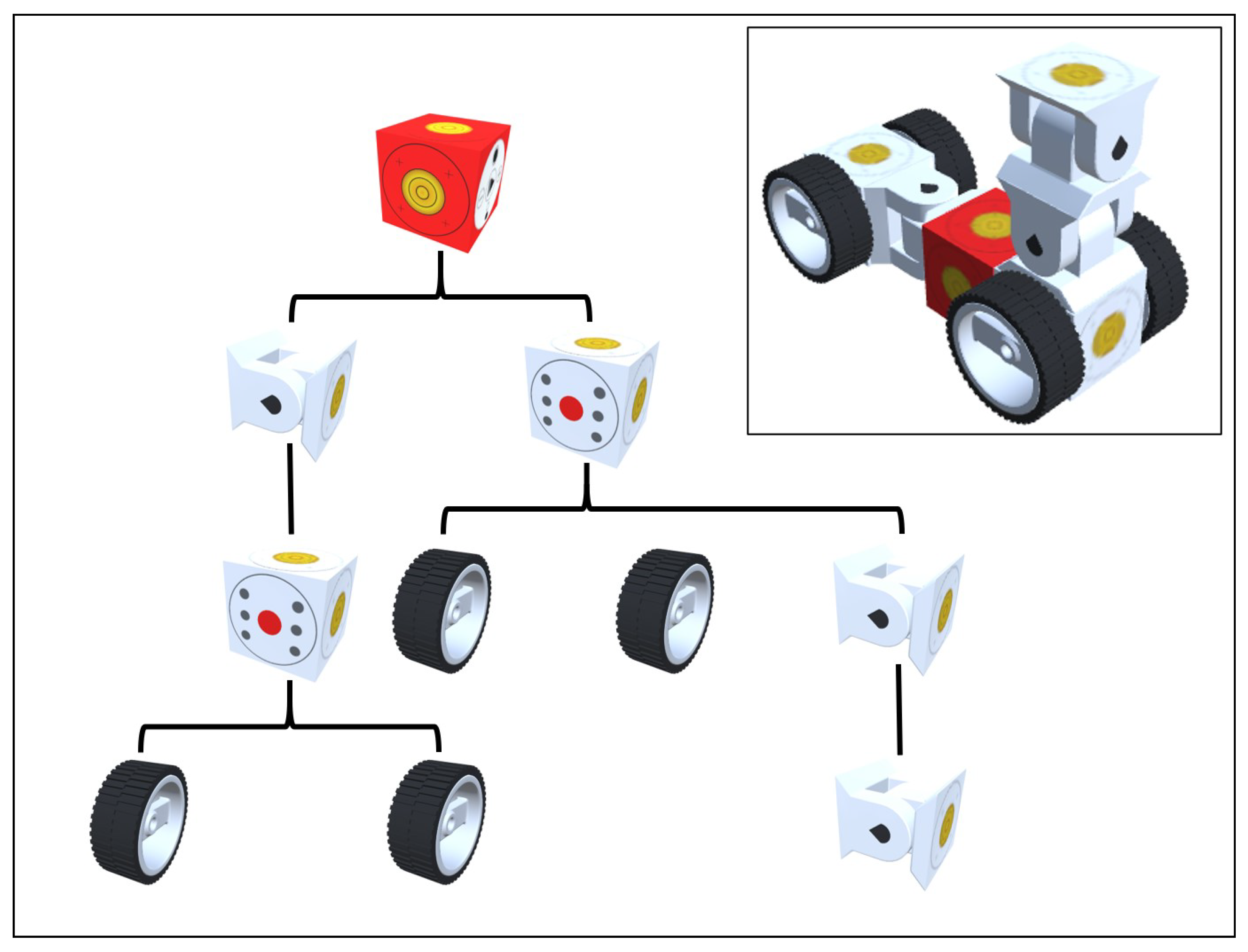
An assembly of elementary modules is represented as a tree structure, wherein each node
n corresponds to an instance of an elementary module, and each edge
e, i.e., an ordered pair of two nodes
, denotes that the child module associated with
m is fitted into the parent module associated with
n (see
Figure 2). In our implementation, the PoweBrain module must be instantiated once at the beginning of an assembly process and it then becomes the root node of the tree. The motor, pivot, and main modules can be instantiated as many times as necessary and become either the internal nodes or the leaf nodes of the tree. The wheel modules must be instantiated in pairs and can only become the leaf nodes of the tree as children of the motor or the main modules. Every non-leaf node in our system can have at most five child nodes because of the inherent restriction imposed by the cubical structure. The relative configuration of each child node with respect to its parent node needs to be specified at the edge connecting between the parent and the child nodes.
We constrain the assembled structure to have at least one motion module, i.e., either the motor module or the pivot module in our implementation, to ensure that the robot can achieve movement. Applying torque to one or more motion modules over a certain duration can allow the robot to move in a specific pattern such as driving to a distant location or twisting its whole body repeatedly. Further, our simulator provides the robot with the ability to sense internal and external states required for achieving the given tasks. The spatial configuration of the robot itsef—encoded as the relative angles of all pivots—is a typical internal state. The relative location of an environment object is an example of the external state, which was used for performing the navigation task in our experiments. In the rest of this manuscript, the term ‘behavior’ is used to indicate how the robot computes the action, i.e., how much torque is applied for each motion module, based on the observed internal and external states.
More specifically, the behavior of each robot in our method is defined as a stochastic policy , which associates each possible state s belonging to a continuous state space S with a probability distribution for sampling an action a from a continuous action space A. After observing the current state at each time step t, the robot determines the corresponding action based on the stochastic policy by sampling from the probability distribution. To generate the actual motion of a robot in our experiments, choosing an action was followed by adjusting the desired angular speeds of the motor modules and the desired angles of pivot modules belonging to the robot. The simulated virtual environment assigns reward to the robot, scoring the performance of the robot with respect to a given goal based on a pre-defined reward function . Further, it moves the robot to a new state by computing the motion of a robot during the time interval between t and based on rigid-body dynamics.
4. Problem Formulation
Given the definitions of structures and behaviors, we can formulate the problem of designing modular robots and present our approach to address the problem in a formal manner. Let
be a structure of a robot, which is represented as the nodes and edges of the assembly tree, and
be its behavior, which is encoded as a set of weights of the deep neural network that associates an arbitrary state with the probability distribution for sampling an action. One plausible formulation of our problem may be to discover the optimal pair of a structure and a behavior
that maximizes the expected cumulative reward
in a simulated virtual environment as follows.
where
and
are the sets of possible structures and behaviors, respectively, and
N and
are the number of episodes and the number of time steps for the
i-th episode, respectively. Howver, it is not practical to optimize both the structure and the behavior simultaneously to find a globally optimal solution, because of the enormous design space over all of the possible structures and behaviors (i.e.,
) and the discrete nature of the structure assembly. Instead, we reformulate our problem as the following bilevel optmization in which the inner optimization in Equation (
3) finds an optimal behavior for a given structure and the outer optimization in Equation (
4) finds an optimal structure that leads to an optimal behavior.
This decoupling allows us to discover a near-optimal solution, i.e., sufficiently good design, in a computationally efficient manner, by solving the inner optimization based on a reinforcement learning algorithm (
Section 5) and the outer optimization based on the genetic algorithm (
Section 6).
5. Learning Behaviors
Once the structure of a robot, , has been defined by a set of modules and their connections, the robot can autonomously learn its behavior, , in a simulated virtual world to achieve a specific goal based on well-known reinforcement learning algorithms. The reward function needs to be defined carefully to measure how well the robot behaves with respect to the task, which requirs iterative improvements through trial and error. It is difficult to obtain a good reward function at the first attempt because an innocent-looking reward function often incentivizes unexpected behaviors. For example, let us consider a sample from our experiments wherein we attempted to train a robot to arrive at an arbitrarily given target location. Rewarding the robot only when it arrived at the target location was not very successful because such rewards were given very rarely, and the robot did not have many opportunities to learn. To encourage the efforts of the robot continuously to allow them to move closer to the target location, we employed a new scheme which compensated for the reduced distance whenever the distance to the target decreased. Contrary to our expectation, the robot learned a policy to maximize rewards by repeating the behavior of approaching and moving away from the target location. We could get the robot to learn properly by adding penalties for moving away and elapsed time.
Once the reward function is appropriately defined, policy-gradient methods can be employed to learn the stochastic policy over continuous action space. The policy
, which is parameterized by
, can be defined as the normal probability density over a real-valued vector action, with its mean and standard deviation given by parametric function approximators that depend on the state, as follows.
where
and
represent the mean and standard deviation, respectively. A policy-gradient method find an optimal parameter
that maximizes the scalar performance measure
by iteratively updating the parameter in the direction of the gradient
, as follows.
In our experiments, we used the proximal policy optimization (PPO) algorithm among various policy-gradient methods for its efficiency. The training of a robot is performed in an episodic manner, in which each new episode starts with a random new configuration of the environment objects related with a given task, and it terminates either when the robot accomplishes the task or after the maximum number of time steps per episode. We calculate and record the cumulative reward for each
i-th episode as follows.
where
denotes the reward received at time step
t and
T denots the length of the
i-th episode, which cannot exceed the maximum number of time steps per episode
.
6. Evolving Structures
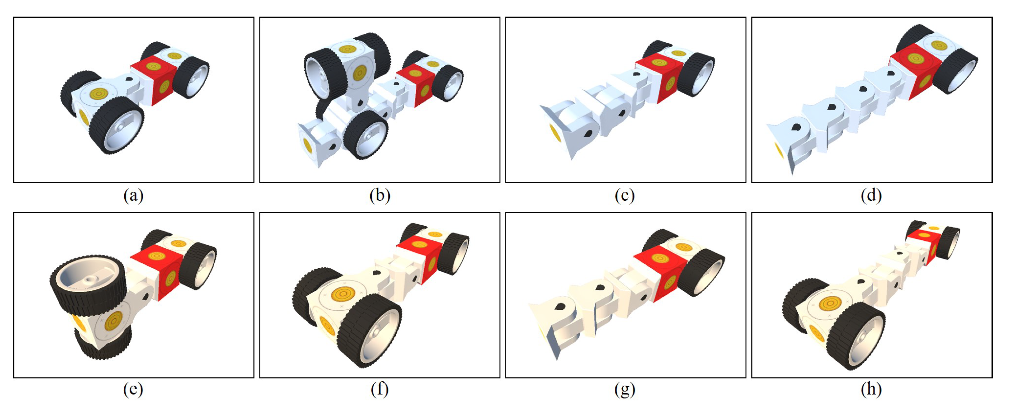
Different structures of a robot agree with different behaviors. Some structures may facilitate highly effective strategies for achieving the given goal, while others may allow only severely ineffective strategies to be found. For example, a four-wheeled structure typically found in real vehicles, as shown in Figure 8a, enables the robot to be efficiently steered towards a target location, which would be quickly learned through reinforcement learning. A snake-like structure with just two wheels, as shown in Figure 8d, hinders the robot from smoothly driving over the environment, and instead corresponds with a wriggling behavior. It is not obvious to determine whether a specific structure is appropriate for a given task only based on intuition. Instead, we quantitatively evaluate the degree of goodness, i.e., fitness, of a specific structure by building that structure, applying a reinforcement learning algorithm to the structure, and then calculating the average of the episodic cumulative reward as the fitness as
where
N denotes the total number of episodes the robot has completed during the training. Equation (
8) is referred to as the learning ability of a robot with respect to a specific goal to be achieved.
Owing to the exponential growth of the number of possible structures based on the number of modules belonging to a structure, the brute-force approach that involves enumerating every possible structure and selecting the best one is not practical. Therefore, we employ the genetic algorithm to find a near-optimal structure,
, practically within the constraints of limited computational resources. Each individual in our implementation of the genetic algorithm corresponds to a candidate robotic structure, which is represented as a tree data structure, as described in
Section 3. A population of a few dozens individuals is randomly generated at the first generation, and then, it is gradually evolved through the succeeding generations based on the fitness evaluation and the crossover operation. The fitness of an individual in our method is defined as the learning ability of its associated robotic structure as explained above, and therefore, the evaluation of the fitness involves a considerable amount of computation for executing the reinforcement learning algorithm. In a typical approach towards the genetic algorithm—the generational approach—the entire population is reproduced and the fitness of every individual is re-evaluated for each new generation. This necessarily leads to a prohibitively long time for convergence. For more rapid convergence, we employ the steady-state approach to the genetic algorithm wherein at most a single new offspring is added to the population replacing a less fit individual for each new generation [
28].
The overview of our evolutionary process for discovering optimal robot designs is shown in
Figure 3. Each step of the process is detailed below.
Generation: A population of initial robots are randomly generated (see
Figure 4). The population size was 20 in our experiments. The random generation of each robot begins by instantiating the root node of a new tree, corresponding to the PowerBrain module in our case. After the generation of the root node, we extend the structure by recursively attaching a new node to every possible side to be extended within a limited depth of recursion. The type of each new node is randomly decided from among the motor, pivot, and main modules. If the motor module is selected, we extend the structure again by attaching two wheel modules symmetrically around the motor module, terminate the recursion, and backtrack to the parent node. Otherwise, we continue the recursion for each side of the newly attached node as long as the current depth of recursion is less than the limit. For each new extension of the structure, we check whether the extended structure is collision free. If self-collsions are identified, we cancel the latest extension and restore the structure to its previous state.
Evaluation: We evaluate the fitness of each new robot by executing the reinforcement learning algorithm with the robot during a limited number of time steps and by measuring the average of the episodic cumulative rewards, as defined in Equation (
8). The number of time steps for learning is set as a relatively small value for every robot in the initial population because the qualities of the initial robots are not expected to be sufficiently high considering their pure randomness. As the evolution proceeds by iteratively replacing second-class robots with smarter ones, we incrementally increases the number of time steps to reveal the potential learning abilities of newer robots more thoroughly.
Reproduction: Instead of recreating the entire population for each new generation, our steady-state approach adopts the policy of gradual one-by-one reproduction. At each generation, we select two robots for reproduction from the existing population based on the fitness proportion selection scheme. In this scheme, which is also known as roulette wheel selection, the probability of selecting a specific individual increases linearly with its fitness level, as defined in the following equation.
New robots are created by recombining the selected two robots based on subtree crossover, which has been popularly used for the genetic programming (see
Figure 5) [
29]. Given trees
and
associated with the selected robots, we randomly choose a pair of internal nodes
and
, whose parent nodes are of the same type, from
and
, respectively, and we swap the two subtrees rooted at
and
to produce a pair of new trees
and
. It is probable that a new tree can yield an invalid robotic structure (e.g., no motion module or self-collision) that needs to be discarded instead of being included in the population. If no new robots are valid, we then reiterate the process of recombination from the beginning. Otherwise, we randomly choose one of the valid new robots as the candidate offspring for the next generation.
Replacement: The candidate offspring born through recombination is not always accepted as a member of the population. We allow only an offspring that fits better than at least one of the existing individuals to be included in the population. To this end, we evaluate the fitness of the candidate offspring by employing the reinforcement learning algorithm as described previously, and we compare its fitness value with the minimum fitness of the current population. If the offspring’s fitness is greater than the minimum, we replace the existing robot of the minimum fitness with the candidate offspring, which will be a new member of the population. Otherwise, we simply discard the candidate offspring and retain the population at this iteration.
7. Experimental Results
We implemented a testbed wherein a population of modular robots could be generated and evolved to adapt to the given task and environment based on our method using C# language in the Unity engine. For the fitness evaulation, we used the implementation of the PPO algorithm included in the Unity Machine Learning Agents Toolkit (ML-Agents) [
30].
We experimented with two different environments while staying on the same task for every robot, i.e., moving one’s body as closely as possible to a target location. A simple environment that comprises a floor and surrounding walls was first experimented with, and then, a cluttered environment, where there were a lot of rocks scattered around the target location, was used for the second experiment (see
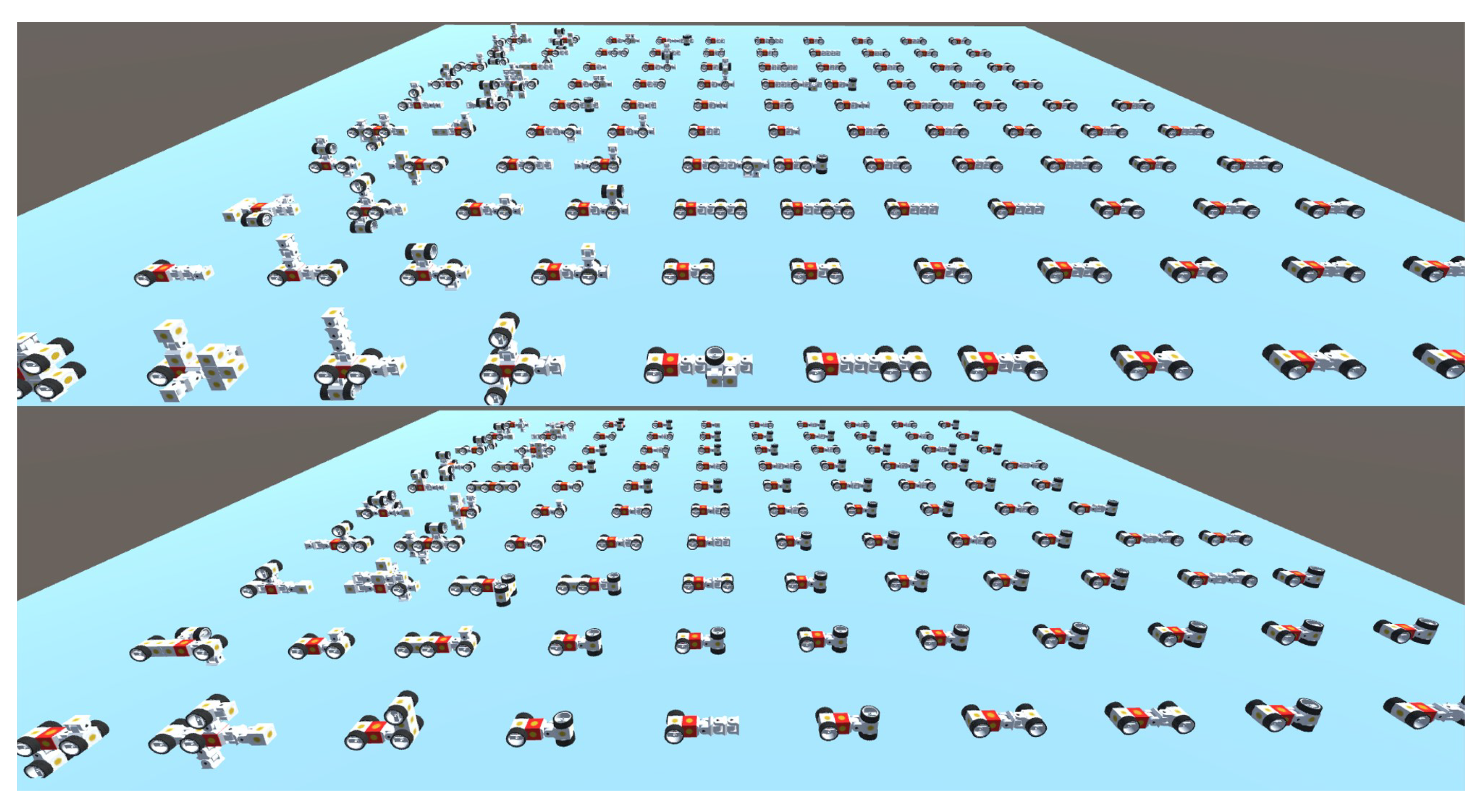
Figure 6). Approximately 100 robots were generated through each experiment, which took about 60 h on a desktop PC equipped with the Intel Core i7-3770 processor (see
Figure 7).
Most setups and parameters in our method remained the same for both experiments, except in terms of the complexity of environments. Initially, for each experiment, a population of 20 robots were randomly generated, whose fitnesses were then evaluated by running the reinforcement learning algorithm and computing the averages of episodic cumulative rewards. The maximum number of time steps for each training session started as 50,000 steps for the initial robots and graually increased up to 250,000 steps for the final robots. For training each robot, we instantiated 12 training areas at the same time, which was allowed by ML-Agents to gather many experiences in parallel and to speed up training as a result.
At the beginning of each training episode for a robot, we located the robot at the center of its training area and chose the target location randomly around the robot such that it was neither too far away from nor too close to the robot. For each time step, the robot observed its current state, performed its action determined by the current policy, and received rewards accordingly. The state was observed as a -dimensional vector, where m and n were the numbers of motors and pivots, respectively, consisting of the linear and angular velocities of the robot (6-D), the direction and distance to the target location (3-D), the current and desired angular speed of each motor (2-D), and the current and desired angle of each pivot (2-D). The action was given as a -dimensional vector, corresponding to the desired angular speeds and the desired angles of motors and pivots, respectively, which were set to their associated parameters for rigid-body simulation in Unity.
Three types of rewards were given to the robot. The first one was a time penalty against the waste of time, i.e., a constant negative reward
, where
was the maximum number of time steps per episode, which was set to 1000 in our experiments. The second one was an incentive for encouraging the behaivor of approaching to the target location, computed by the following equation.
where
and
represent the closest distance between the robot and the target location at the current and the previous time step, respectively, and
L denotes the length of a side of the training area used for normalizing the reward value. The bracketed sub-expression on the right is a weighing factor that assigns a higher reward as the robot comes closer to the target. In contrast to the first and second types of rewards assigned at every time step, the last one is an award of
, provided only if the robot successfully completes the task—coming sufficiently close to the target location—consequently terminating the ongoing episode and restarting a new one. Even in the case that the robot was far from being successful, each episode was eventually terminated when the current time step reached the maximum number of time steps per episode
.
7.1. Results from Clean Environment
The top of
Figure 7 shows robots evolved in the clean environment. Starting from a large variety of arbitrarily structured robots, the population eventually converged to two or three representative structures optimized for planar locomotion, such as the ones in the upper row of
Figure 8.
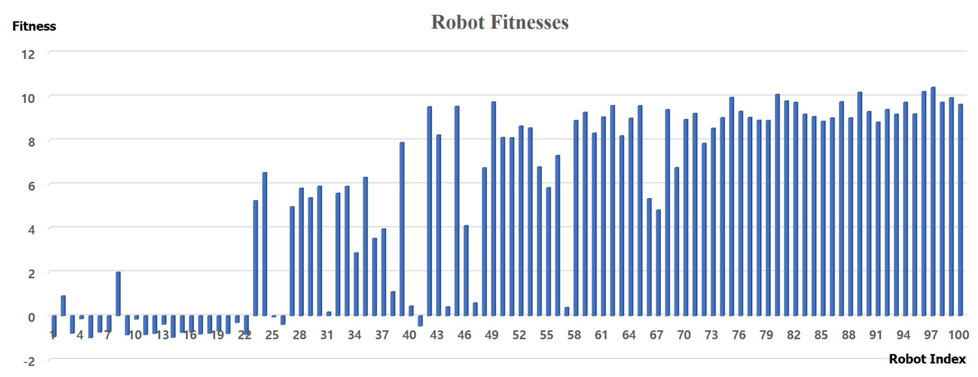
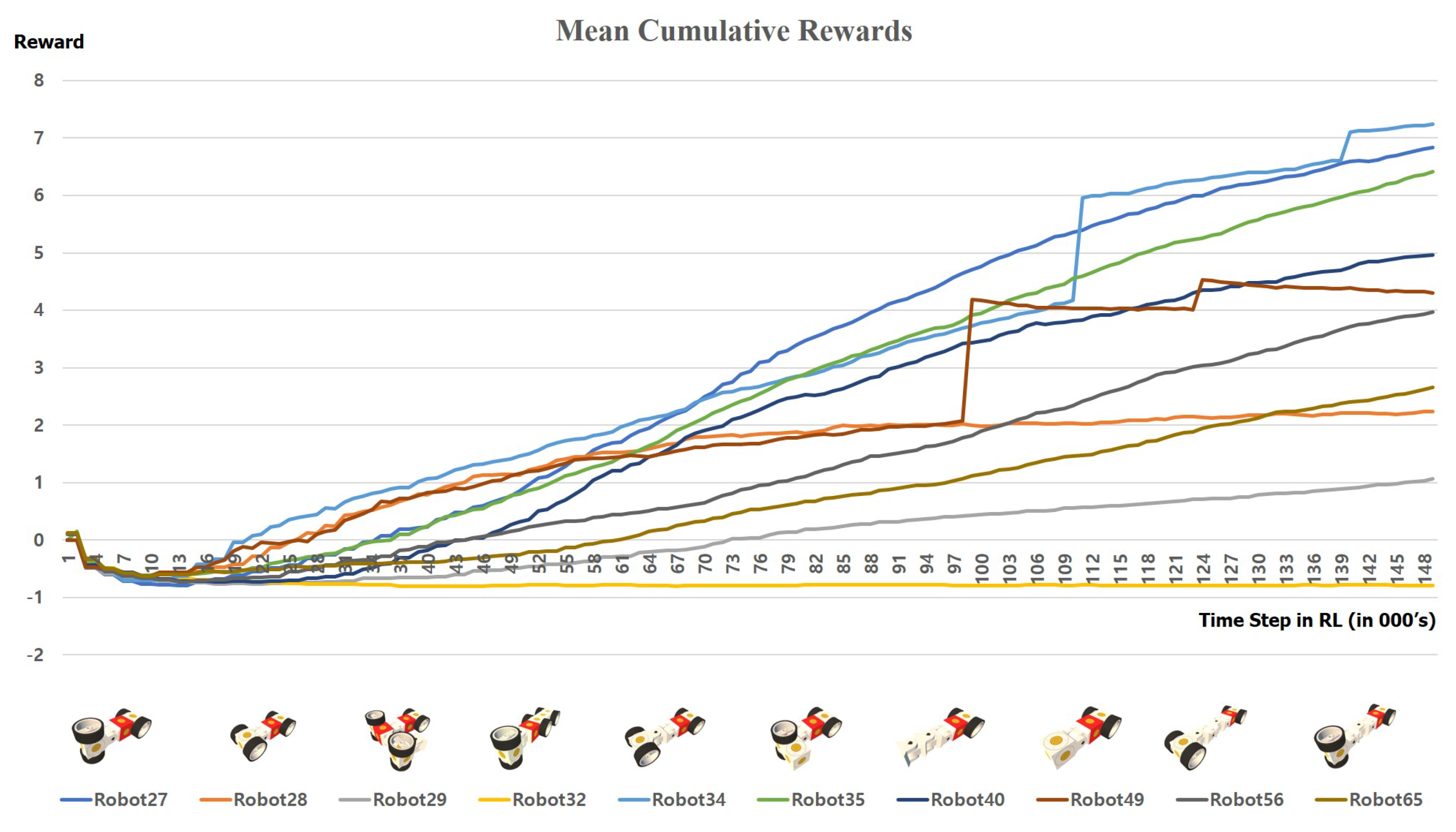
Figure 9 exhibits how the fitnesses (averages of episodic cumulative rewards) increases in training for a diversity of different structures. Some structures seems to facilitate the acquisition of efficient strategies, yielding rapid growths of fitnesses, whereas others seems to impose limitations in learning, leading to little growths of ones. Most of the robots discovered after 50 reproductions obtained satisfactory fitnesses, as depicted in
Figure 10.
The compact four-wheeled structure shown in
Figure 8a, which includes a pivot for left and right turn in the middle, proves to be the best solution for quickly steering the robot to a target location. However, the advantage of our method can be found in somewhat unexpected structures that produces interesting and inspiring behaviors. The robot in
Figure 8b is not the best driver, but it uses a unique mechanism for turning abruptly by striking the ground with the hammer-like upper parts. Although the robots in
Figure 8c,d have two-wheeled structures, they can effectively navigate the environment by exhibiting inchworm-like and snake-like behaviors, respectively. Such results demonstrate the key strength of our method in discovering a variety of effective combinations of structures and behaviors from a vast design space.
7.2. Results from Cluttered Environment
The bottom of
Figure 7 shows robots evolved in the cluttered environment. In the clean environment, the robots primarily resort to planar translation by wheels and horizontal rotation by pivots to turn sideways, which are not effective for overcoming the obstruction of rocks scattered around the target location. In contrast, structures evolved in the cluttered environment invariably include one or more sub-structures that facilitate up-and-down motions, mostly connected by pivots rotating about horizontal axes, as shown in the lower row of
Figure 8, which allow the robots to move over the obstructions more easily by climbing over or pushing away nearby rocks.
Figure 11 shows the fitness graphs of some robots that exhibit dramatic jumps at two separate points in training, although the fitnesses of most robots increase smoothly like those in the previous experiment in the clean environment. Our current interpretation for such discontinuous events is that motion parameters for the corresponding structures require highly sensitive adjustment for passing over obstacles; the jumps in the learning curves represent sudden discoveries of precise parameter values. This interpretation is partially supported by the fact that the shapes and sizes of the rocks used in the experiment are classified into five fixed types instead of being variable arbitrarily. There may be some magic values for the motion parameters to precisely overcome only these five types of rocks.
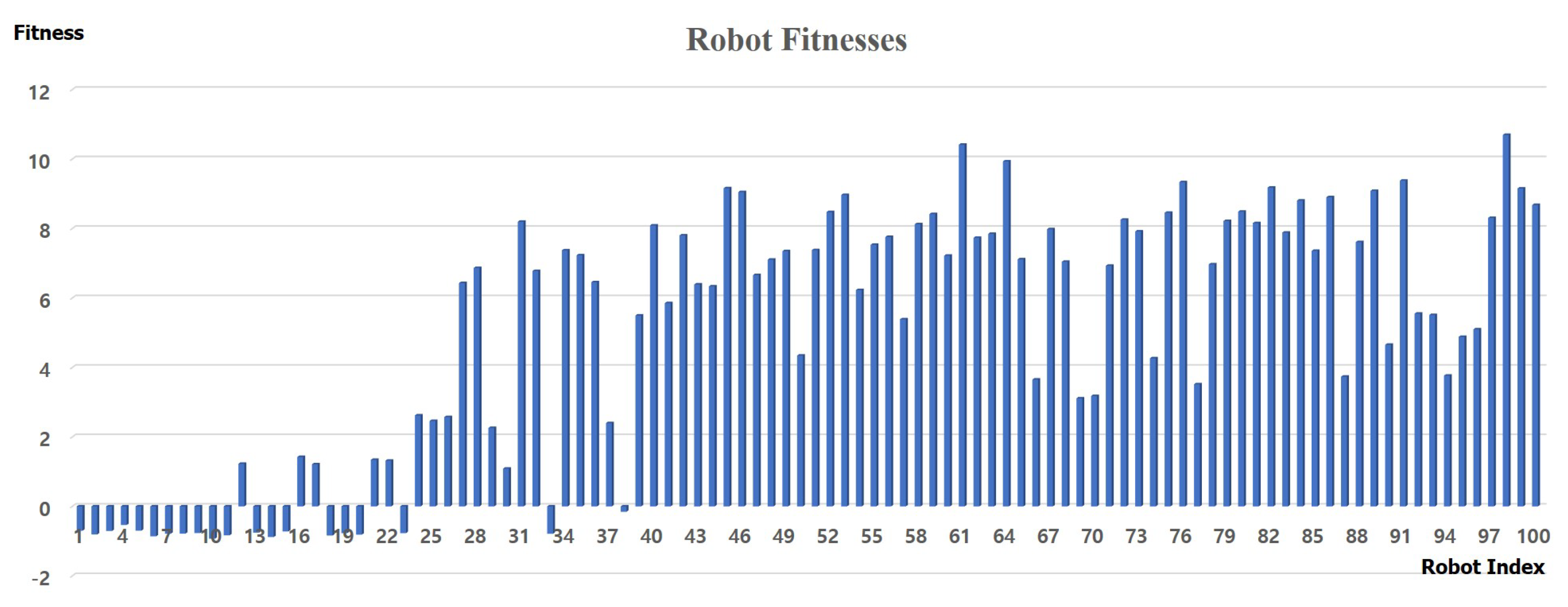
Figure 12 shows that the cluttered environment certainly elevates the difficulty level for task completion. Even in the later generations, a considerable number of newborn robots suffer from relatively low fitness values between 3 and 5, in comparison with that the most of the later generations in the clean environment reach about 10 in their fitnesses. Similarly to the steep growths of fitnesses mentioned above, the drastic change in the fitnesses over successive generations can be interpreted as the result of the senstivitity of learning ability to the structural modification of a robot. That is, it is less probable to produce a competent child robot from two compenent parents than in the clean environment because a slight modification of a robotic structure, such as the removal of a pivot enabling up-and-down motion, can significantly degrade the performance of the robot in the cluttered environment.
Further, there is a clear winner in this experiment, which is the twisted four-wheeld robot in
Figure 8e, whose structure is prevalent in the later generations of the evolution. In appearance, it looks similar to the best robot for the clean enviornment in
Figure 8a except for the orthogonal rotation of the half of its body. However, its strategic approach to move to a target location is completely novel and beyond ordinary imagination. It uses the hammer-like part—a pair of horizontal wheels attached to the top and bottom of the main module in parallel with the floor—very effectively for more than one purpose. The hammer is used as if it is a leg of an animal to relocate the body forward while raising the body slightly upward from the ground to allow the robot to pass over the rocks on the ground in a relatively easy way. Additionally, the hammer is utilized for steering the moving direction of the robot to the left or right by turning its wheels in the clockwise or the counter-clockwise direction while sticking the bottom wheel to the ground.
Other structures shown in
Figure 8f–h display various effective strategies for locomotion in a cluttered environment, which is usually based on the three-dimensional twisting of their bodies. In terms of uniqueness, the structure in
Figure 8g shows the most interesting behavior. The robot uses the chain-like structure as if it is a sweeping tool by swaying the chain from side to side, which can effectively push the rocks around. One typical problem found in these twistable structures is that they can be often turned over when they are caught in rocks and attempt to move forward forcibly. Because we did not allow a robot to observe its upward direction, the robot could not learn how to recover its original state once it turned over in our experiments.
8. Discussion
One interesting hypothesis from our observations over the experimental results is that the early tendencies of how rapidly or slowly the mean cumulative rewards increase with respect to the time steps determine the eventual fitnesses or rankings at the later phases. In the experiment with the clean environment, the final rankings of the 10 robots measured at the 150,000th step are almost the same with the early rankings measured at about the 30,000th step, as shown in
Figure 9. The experimental result from the cluttered environment, shown in
Figure 11, seems to object to such a hypothesis because the rankings of some robots change drastically at relatively later time steps (around the 100,000-th step). However, such reversals of the rankings can be predicted earlier to a ceratin degree if we consider the time derivates of the mean cumulative rewards as well. For example, although the early ranking of the
robot 40 is very low, around 8th place at the 30,000th step, the slope of its graph is relatively steep and its final ranking goes up to 4th place. On the other hand, the
robot 28, an early winner in the cluttered environment, exhibits a relatively gentle slope at the early stage and its final ranking drops to 8th place. We are not yet prepared for either accepting or rejecting this hypothesis due to the insufficient amount of experimental data, but believe that it is a promising research direction to develop an efficient method for predicting the potential ability of a robotic structure based on this hypothesis.
Our experimental results successfully show that our method is effective in discovering sufficiently good solutions—compact, powerful, and inspirational structures and behaviors—by exploring only a tiny fraction of the entire design space (at most 100 robotic structures). To comprehend how appropriately the genetic algorithm and the reinforcement learning are interlinked together to solve the bilevel optimization in Equations (
3) and (
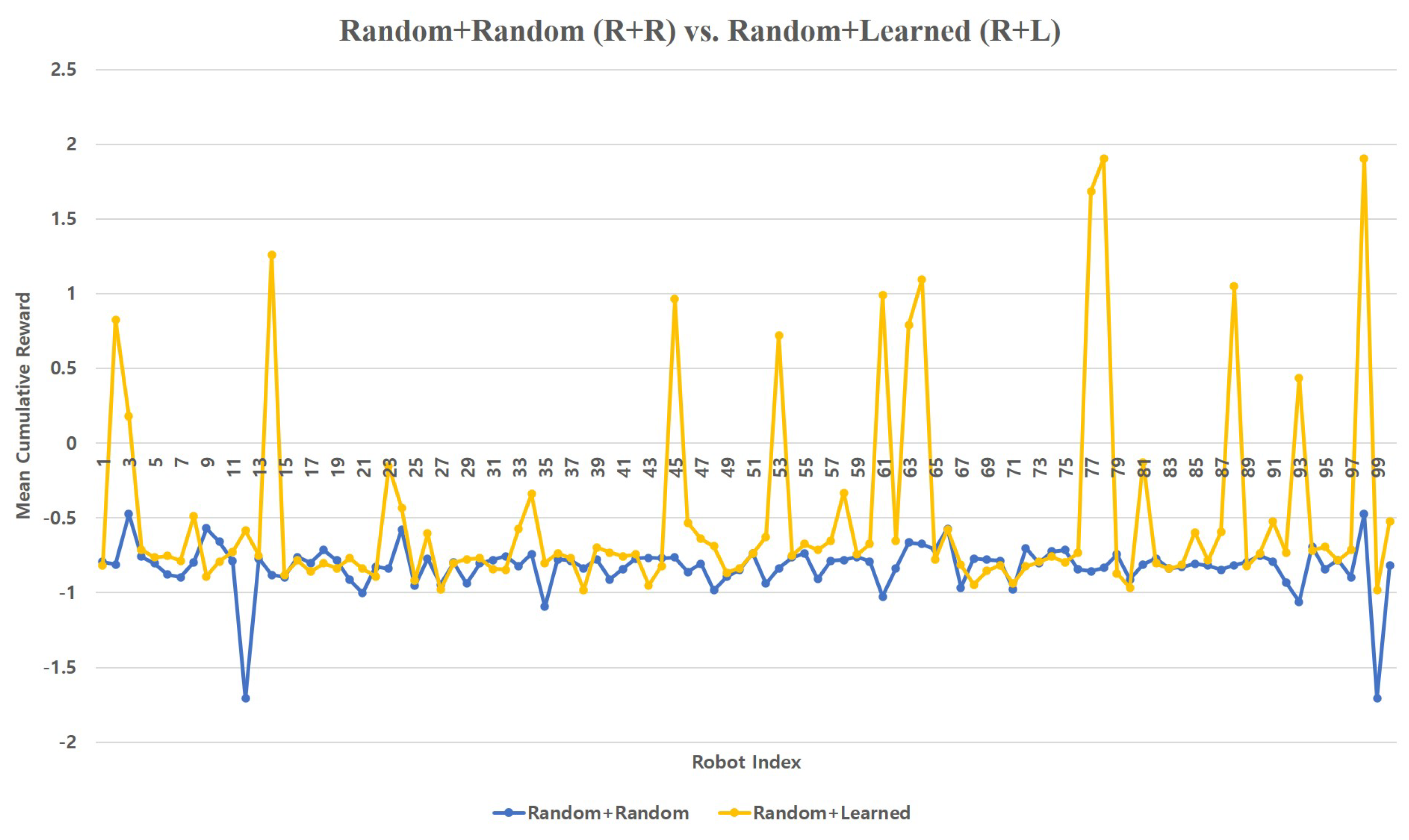
4), we performed an additional experiment with four different optimization methods and compared their results quantitatively. The first method was to explore the entire design space in a fully stochastic way by assigning a random structure and a random behavior for each new robot (R+R). The second and the third methods were similar to the first method in that they partly resorted to the stochastic exploration of either structures or behaviors. Specifically, the second method was a combination of the random exploration of structures and the reinforcement learning of behaviors (R+L), and the third one was a combination of the genetic evolution of structures and the random initialization of behaviors (E+R). Lastly, the fourth method exactly corresponded to our method, i.e., a combination of the genetic evolution of structures and the reinforcement learning of behaviors (E+L). We generated about 100 robots by each method and collected the final mean cumulative reward of each robot. Differently from the previous experiments, the maximum number of time steps was fixed at 30,000 steps, which was a relatively short duration but was enough for comparing the performances of optimization methods.
The ‘R+R’ method can be regarded as a baseline method because it just randomly samples from the entire design space. The graph from ‘R+R’ (blue), whose vertical coordinates mostly stay between
and
, reveals the intrinsic difficulty of our optimization problem (see
Figure 13,
Figure 14 and
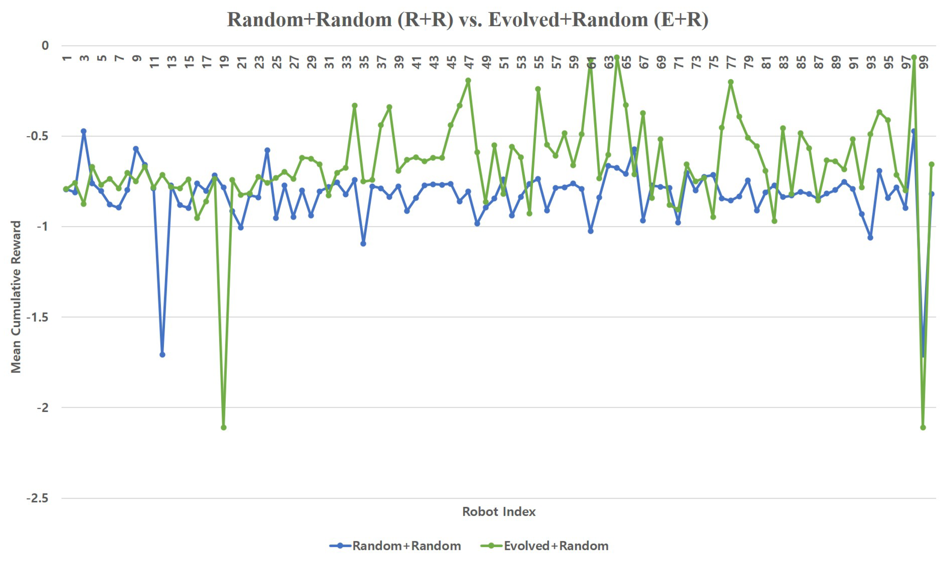
Figure 15). In other words, it is hardly probable to obtain even a reasonable level of robot design just by chance in our problem domain. The ‘E+R’ (green) compared to the ‘R+R’ informs that genetic evolution by itself does not seem to contribute much to the performance of optimization (see
Figure 13). The maximum of the mean cumulative rewards from ‘E+R’ (
) is a bit greater than the maximum from ‘R+R’ (
), but still cannot be regarded as a practically meaningful score. An evident improvement is found in the ‘R+L’ graph (yellow), in which some exceptionally high rewards (
at a maximum) are scatteringly distributed (see
Figure 14). This result implies that it is quite possible to discover potentially good robot designs whose performances can be dramatically enhanced by training in a stochastic manner. However, the low average (
) and the small standard deviation (
) from ‘R+L’ indicate that most designs remain in a practically incompetent area in the design space and it is difficult to expect continuous improvement in structures. The ‘E+L’, corresponding to our method, clearly outperforms all other methods and displays substantial improvement from the ‘R+L’ (see
Figure 15). Despite that the genetic evolution by itself contributes not much, combining it with the behavior optimization based on the reinforcement learning proves to be a highly effective method that not only produces highly competent designs (the maximum of the mean cumulative reward:
), much better than the best one from ‘R+L’, but also explores the promising area of the design space extensively (the average: 0.50, the std. dev.: 1.07). These results demonstrate that our method effectively reduces the design space based on the separation of structural and behavioral optimizations and efficiently finds prospective robotic structures that can potentially lead to near-optimal behaviors if trained sufficiently.
9. Conclusions
We presented a method for discovering effective designs of modular robots using the genetic algorithm for evolving the structures of robots and applying the reinforcement learning algorithm to the evolved structures for training the behaviors of robots. The separation of the structural evolution and behavioral learning reduces the design space significantly in comparison with typical methods developed in evolutionary robotics, which makes our method practically applicable to non-trivial design problems in the real world. The circular interdependency between the evolution and the learning allows the structures and the behaviors to be optimized in a tighly coupled manner, which eventually produces the optimal structures that can potentially lead to the near-optimal behaviors once trained sufficiently.
The usefulness of our method was demonstrated through two successive experiments with the same task and different environments. Because of the advantantages of the evolutionary approach, we obtained robotic structures that were tailored to the property of each environment. Thus, the optimal structures evolved in one environment were clearly different from the ones evolved in the other. The reinforcement learning algorithm enabled the behavior for each robotic structure to be optimized efficiently so that the potential ability of the given structure could be developed to accomplish the given task in its best possible manner. The comparative experiments described in
Section 8 reveal the key advantage of our method that the enormous design space for robot design can be effectively explored and sufficiently good designs can be efficiently discovered based on our bilevel optimization.
A key limitation of our method is that it requires a considerable amount of time to evaluate the fitness of each structure for executing the reinforcement learning algorithm. Several performance optimization techniques combined with the utilization of one or more GPUs can certainly help reduce the time for fitness evaluation to ensure practicality. However, in a more fundamental way, we expect that deep learning algorithms can be employed to predict the fitness of a structure instantly based only on the short sequences of the cumulative rewards during a small number of initial time steps. As described in
Section 8, the graphs of mean cumulative rewards in
Figure 9 and
Figure 11 show that their initial patterns are closely related with the final fitness values. Based on the acceleration of our method obtained using the deep learning algorithms, we aim at designing considerably more complicated robots than the ones produced by our experiments in this study, and possibly with a larger diversity of elementary modules and a hierarchy of multiple behaviors. For example, evolving animal-like robots which incorporate locomotion mechanisms as well as visual perception circuits based on a collection of basic vision modules, such as an edge detector, could be one interesting future work.
Author Contributions
Conceptualization, K.H.L.; methodology, J.H.P. and K.H.L.; software, J.H.P.; validation, J.H.P. and K.H.L.; formal analysis, J.H.P. and K.H.L.; investigation, J.H.P. and K.H.L.; resources, J.H.P. and K.H.L.; data curation, J.H.P. and K.H.L.; writing—original draft preparation, K.H.L.; writing—review and editing, K.H.L.; visualization, K.H.L.; supervision, K.H.L.; project administration, K.H.L.; funding acquisition, K.H.L. All authors have read and agreed to the published version of the manuscript.
Funding
This work was supported by the National Research Foundation of Korea(NRF) grant funded by the Korea government(MSIT) (No. NRF-2018R1D1A1B07043995).
Institutional Review Board Statement
Not applicable.
Informed Consent Statement
Not applicable.
Data Availability Statement
Data available on request.
Acknowledgments
The work reported in this paper was conducted during the sabbatical year of Kwangwoon University in 2018.
Conflicts of Interest
The authors declare no conflict of interest.
References
- Guizzo, E. By leaps and bounds: An exclusive look at how boston dynamics is redefining robot agility. IEEE Spectr. 2019, 56, 34–39. [Google Scholar] [CrossRef]
- Sung, J.-Y.; Guo, L.; Grinter, R.E.; Christensen, H.I. My Roomba is Rambo: Intimate home appliances. In International Conference on Ubiquitous Computing; Springer: Berlin/Heidelberg, Germany, 2007. [Google Scholar]
- Doncieux, S.; Bredeche, N.; Mouret, J.-B.; Eiben, A.E. Evolutionary robotics: What, why, and where to. Front. Robot. AI 2015, 2, 1–18. [Google Scholar] [CrossRef]
- Tinkerbots Modular Robotics Kit. Available online: http://www.tinkerbots.de (accessed on 12 March 2021).
- Bermano, A.H.; Bermano, T.; Rusinkiewicz, S. State of the art in methods and representations for fabrication-aware design. Comput. Graph. Forum 2017, 36, 509–535. [Google Scholar] [CrossRef]
- Zhu, L.; Xu, W.; Snyder, J.; Liu, Y.; Wang, G.; Guo, B. Motion-guided mechanical toy modeling. ACM Trans. Graph. 2012, 31, 127:1–127:10. [Google Scholar] [CrossRef]
- Coros, S.; Thomaszewski, B.; Noris, G.; Sueda, S.; Forberg, M.; Sumner, R.W.; Matusik, W.; Bickel, B. Computational design of mechanical characters. ACM Trans. Graph. 2013, 32, 83:1–83:12. [Google Scholar] [CrossRef]
- Ceylan, D.; Li, W.; Mitra, N.J.; Agrawala, M.; Pauly, M. Designing and fabricating mechanical automata from mocap sequences. ACM Trans. Graph. 2013, 32, 186:1–186:11. [Google Scholar] [CrossRef]
- Thomaszewski, B.; Coros, S.; Gauge, D.; Megaro, V.; Grinspun, E.; Gross, M. Computational design of linkage-based characters. ACM Trans. Graph. 2014, 33, 64:1–64:9. [Google Scholar] [CrossRef]
- Megaro, V.; Thomaszewski, B.; Nitti, M.; Hilliges, O.; Gross, M.; Coros, S. Interactive design of 3D-printable robotic creatures. ACM Trans. Graph. 2015, 32, 216:1–216:9. [Google Scholar] [CrossRef]
- Geilinger, M.; Poranne, R.; Desai, R.; Thomaszewski, B.; Coros, S. Skaterbots: Optimization-based design and motion synthesis for robotic creatures with legs and wheels. ACM Trans. Graph. 2018, 37, 160:1–160:12. [Google Scholar] [CrossRef]
- Zhu, Z.; Pan, Y.; Zhou, Q.; Lu, C. Event-triggered adaptive fuzzy control for stochastic nonlinear systems with unmeasured states and unknown backlash-like hysteresis. IEEE Trans. Fuzzy Syst. 2020. [Google Scholar] [CrossRef]
- Roman, R.-C.; Precup, R.-E.; Petriu, E.M. Hybrid data-driven fuzzy active disturbance rejection control for tower crane systems. Eur. J. Control 2021, 58, 373–387. [Google Scholar] [CrossRef]
- Goldberg, D.E. Genetic Algorithms in Search, Optimization and Machine Learning; Addison-Wesley: Hoboken, NJ, USA, 1989. [Google Scholar]
- Baioletti, M.; Milani, A.; Santucci, V. Variable neighborhood algebraic differential evolution: An application to the linear ordering problem with cumulative costs. Inf. Sci. 2020, 507, 37–52. [Google Scholar] [CrossRef]
- Sims, K. Evolving virtual creatures. In Proceedings of the ACM SIGGRAPH 1994, Orlando, FL, USA, 24–29 July 1994; pp. 15–22. [Google Scholar]
- Funes, P.; Pollack, J. Evolutionary body building: Adaptive physical designs for robots. Artif. Life 1998, 4, 337–357. [Google Scholar] [CrossRef]
- Lipson, H.; Pollack, J.B. Automatic design and manufacture of robotic lifeforms. Nature 2000, 406, 974–978. [Google Scholar] [CrossRef] [PubMed]
- Kamimura, A.; Kurokawa, H.; Yoshida, E.; Murata, S.; Tomita, K.; Kokaji, S. Automatic locomotion design and experiments for a modular robotic system. IEEE ASME Trans. Mechatron. 2005, 10, 314–325. [Google Scholar] [CrossRef]
- Duarte, M.; Gomes, J.; Oliveira, S.M.; Christensen, A.L. Evolution of repertoire-based control for robots with complex locomotor systems. IEEE Trans. Evol. Comput. 2018, 2, 314–328. [Google Scholar] [CrossRef]
- Larik, A.; Haider, S. A framework based on evolutionary algorithm for strategy optimization in robot soccer. Soft Comput. 2019, 23, 7287–7302. [Google Scholar] [CrossRef]
- Alattas, R.J.; Pater, S.; Sobh, T.M. Evolutionary modular robotics: Survey and analysis. J. Intell. Robot. Syst. 2019, 95, 815–828. [Google Scholar] [CrossRef]
- Lund, H.H. Co-evolving control and morphology with LEGO robots. In Morpho-functional Machines: The New Species; Springer: New York, NY, USA, 2003; pp. 59–79. [Google Scholar]
- Ha, S.; Coros, S.; Alspach, A.; Kim, J.; Yamane, K. Joint optimization of robot design and motion parameters using the implicit function theorem. Robot. Sic. Syst. 2017, 13. [Google Scholar]
- Schaff, C.; Yunis, D.; Charkrabarti, A.; Walter, M.R. Jointly learning to construct and control agents using deep reinforcement learning. In Proceedings of the 2019 International Conference on Robotics and Automation (ICRA), Montreal, QC, Canada, 20–24 May 2019; pp. 9798–9805. [Google Scholar]
- Kober, J.; Bagnell, J.A.; Peters, J. Reinforcement learning in robotics: A survey. Int. J. Robot. Res. 2013, 32, 1238–1274. [Google Scholar] [CrossRef]
- Schulman, J.; Wolski, F.; Dhariwal, P.; Radford, A.; Klimov, O. Proximal policy optimization algorithms. arXiv 2017, arXiv:1707.06347. [Google Scholar]
- Blum, C.; Roli, A. Metaheuristics in combonational optimization: Overview and conceptual comparison. ACM Comput. Surv. 2003, 35, 268–308. [Google Scholar] [CrossRef]
- Banzhaf, W.; Francone, F.D.; Keller, R.E.; Nordin, P. Genetic Programming: An Introduction: On the Automatic Evolution of Computer Programs and Its Applications; Morgan Kaufmann: San Francisco, CA, USA, 1998. [Google Scholar]
- Juliani, A.; Berges, V.; Teng, E.; Cohen, A.; Harper, J.; Elion, C.; Goy, C.; Gao, Y.; Henry, H.; Mattar, M.; et al. Unity: A General Platform for Intelligent Agents. arXiv 2020, arXiv:1809.02627. [Google Scholar]
Figure 1.
PowerBrain, motor, main, wheel, and pivot modules (in a clockwise direction from the left top).
Figure 1.
PowerBrain, motor, main, wheel, and pivot modules (in a clockwise direction from the left top).
Figure 2.
An example robot structure. The four-wheeled robot on the upper right is represented as the tree structure.
Figure 2.
An example robot structure. The four-wheeled robot on the upper right is represented as the tree structure.
Figure 3.
Overview of our evolutionary design process. The blue bar below each robot represents the fitness of the robot. The robots in the red regions represent the selected and the replaced robots.
Figure 3.
Overview of our evolutionary design process. The blue bar below each robot represents the fitness of the robot. The robots in the red regions represent the selected and the replaced robots.
Figure 4.
An example of an initial population of random robots.
Figure 4.
An example of an initial population of random robots.
Figure 5.
An example of the crossover operation. The sub-structures in the yellow and blue regions are pruned from the left two parent robots, and then are recombined to produce the child structure on the right.
Figure 5.
An example of the crossover operation. The sub-structures in the yellow and blue regions are pruned from the left two parent robots, and then are recombined to produce the child structure on the right.
Figure 6.
Training candidate robotic structures in the clean environment (left) and the cluttered environment (right).
Figure 6.
Training candidate robotic structures in the clean environment (left) and the cluttered environment (right).
Figure 7.
The resulting structures evolved from the clean environment (top) and the cluttered environment (bottom).
Figure 7.
The resulting structures evolved from the clean environment (top) and the cluttered environment (bottom).
Figure 8.
Noteworthy robots evolved from the clean environment (top) and the cluttered environment (bottom).
Figure 8.
Noteworthy robots evolved from the clean environment (top) and the cluttered environment (bottom).
Figure 9.
Changes of the mean cumulative rewards during the training in the clean environment.
Figure 9.
Changes of the mean cumulative rewards during the training in the clean environment.
Figure 10.
The fitnesses of all robots generated by our evolutionary process in the clean environment.
Figure 10.
The fitnesses of all robots generated by our evolutionary process in the clean environment.
Figure 11.
Changes of the mean cumulative rewards during the training in the cluttered environment.
Figure 11.
Changes of the mean cumulative rewards during the training in the cluttered environment.
Figure 12.
The fitnesses of all robots generated by our evolutionary process in the cluttered environment.
Figure 12.
The fitnesses of all robots generated by our evolutionary process in the cluttered environment.
Figure 13.
Comparing ‘R+R’(random structure combined with random behavior) and ‘E+R’(evolved structure combined with random behavior).
Figure 13.
Comparing ‘R+R’(random structure combined with random behavior) and ‘E+R’(evolved structure combined with random behavior).
Figure 14.
Comparing ‘R+R’(random structure combined with random behavior) and ‘R+L’(random structure combined with learned behavior).
Figure 14.
Comparing ‘R+R’(random structure combined with random behavior) and ‘R+L’(random structure combined with learned behavior).
Figure 15.
Comparing ‘R+R’(random structure combined with random behavior) and ‘E+L’(evolved structure combined with learned behavior).
Figure 15.
Comparing ‘R+R’(random structure combined with random behavior) and ‘E+L’(evolved structure combined with learned behavior).
| Publisher’s Note: MDPI stays neutral with regard to jurisdictional claims in published maps and institutional affiliations. |
© 2021 by the authors. Licensee MDPI, Basel, Switzerland. This article is an open access article distributed under the terms and conditions of the Creative Commons Attribution (CC BY) license (http://creativecommons.org/licenses/by/4.0/).
