A New Application of Gauss Quadrature Method for Solving Systems of Nonlinear Equations

Abstract

In this paper, we introduce a new three-step Newton method for solving a system of nonlinear equations. This new method based on Gauss quadrature rule has sixth order of convergence (with $n=3$). The proposed method solves nonlinear boundary-value problems and integral equations in few iterations with good accuracy. Numerical comparison shows that the new method is remarkably effective for solving systems of nonlinear equations.

1. Introduction

In numerical analysis and other branches of scientific interests, solving a system of nonlinear equations by means of computational methods has always been very well motivated and convincing for researchers. For a system of nonlinear equations:

$$P\left(S\right)={\left(p_1\left(S\right),p_2\left(S\right),\cdots ,p_n\left(S\right)\right)}^T=0,$$

(1)

where $S={(s_1,s_2,\cdots ,s_n)}^T$ and $P:D\subseteq {\mathbb{R}}^n⟶{\mathbb{R}}^n$ is a nonlinear system, and $p_i,i=1,2,\cdots ,n:$$D\subseteq {\mathbb{R}}^n⟶\mathbb{R}$ is a nonlinear mapping. The solution of the nonlinear system of equations in (1) may be defined as the process of finding a vector $S^{*}={(s_1^{*},s_2^{*},\cdots ,s_n^{*})}^T$ such that $P\left(S^{*}\right)=0.$ The classical Newton method is one of the most commonly used iterative methods:

$$S^{(k+1)}=S^k-P^{\prime }{\left(S^{\left(k\right)}\right)}^{-1}P\left(S^{\left(k\right)}\right)(k=0,1,2,\cdots ),$$

where $P^{\prime }\left(S^{\left(k\right)}\right)$ is the Jacobian matrix of the nonlinear function $P\left(S\right)$ in the kth iteration at the point $S^{\left(k\right)}$ (see [1,2,3]). Newton’s method quadratically converges to the solution $S^{*}$ if the function P is continuous and differentiable. In recent years, several methods have been developed to analyze the solution of systems of nonlinear equations to improve interaction by using the quadrature formulas and fractional iterative method in the literature (see [4,5,6,7,8,9,10,11,12]). In particular, Codero and Torregrosa [9] developed the third-order Newton–Simpson method as follows:

$$S^{(k+1)}=S^{\left(k\right)}-6{\left[P^{\prime }\left(S^{\left(k\right)}\right)+4P^{\prime }\left(\frac{S^{\left(k\right)}+Y^{\left(k\right)}}{2}\right)+P^{\prime }\left(Y^{\left(k\right)}\right)\right]}^{-1}P\left(S^{\left(k\right)}\right),$$

(2)

and the Open Newton method:

$$\begin{array}{cc}\hfill S^{(k+1)}& =S^{\left(k\right)}-3[2P^{\prime }\left(\frac{S^{\left(k\right)}+3Z^{\left(k\right)}}{4}\right)-P^{\prime }\left(\frac{S^{\left(k\right)}+Z^{\left(k\right)}}{2}\right)\hfill \\ \hfill & +2P^{\prime }\left(\frac{3S^{\left(k\right)}+Z^{\left(k\right)}}{4}\right){]}^{-1}P\left(S^{\left(k\right)}\right),\hfill \end{array}$$

(3)

where $Z^{\left(k\right)}$ represents the Newton approximation. Khirallah and Hafiz [13] suggested a cubically convergent method using the four-point Newton–Cotes formula for solving systems of nonlinear equations as follows:

$$\begin{array}{cc}\hfill S^{(k+1)}& =S^{\left(k\right)}-8[P^{\prime }\left(S^{\left(k\right)}\right)+3P^{\prime }\left(\frac{2S^{\left(k\right)}+Z^{\left(k\right)}}{2}\right)+3P^{\prime }\left(\frac{S^{\left(k\right)}+2Z^{\left(k\right)}}{2}\right)\hfill \\ \hfill & +P^{\prime }\left(Z^{\left(k\right)}\right){]}^{-1}P\left(S^{\left(k\right)}\right).\hfill \end{array}$$

(4)

The quadrature rule is used to approximate the definite integral of a function. The general form of a quadrature rule is given by [14]

$$Q={\int }_a^{b}v\left(r\right)s\left(r\right)dr\simeq Q_m=\sum _{i=0}^m{w}_{i}s\left(r_i\right)$$

where $v\left(r\right)$ is a weight function, $w_i,i=0,1,2,\dots m$ are coefficients (weights). $r_i$ are points of the rule and s is a given function integrable on the interval $[a,b]$ with the weight function v.

Motivated and inspired by the research going on in this area, we have introduced a new iterative for solving nonlinear equations. Several numerical examples are considered to show the effectiveness of the proposed method. The new iterative method shows the compatibility of numerical results with the scheme’s theoretical analysis. We have solved nonlinear boundary-value problems by using the proposed method. Our method gives better results than the other methods and converges more rapidly to the solution. Section 5 concludes the paper.

2. Three-Step Newton Method

Let $P:D\subseteq {\mathbb{R}}^n⟶{\mathbb{R}}^n$, be s-times Fréchet differentiable function on a convex set $D\subseteq {\mathbb{R}}^n$. Using the Mean-Value Theorem of multi-variable vectors function $P\left(S^{\left(k\right)}\right)$ (see [1]), we have

$$P\left(S\right)-P\left(S^{\left(k\right)}\right)={\int }_0^1{P}^{\prime }\left(S^{\left(k\right)}+r(S-S^{\left(k\right)})\right)(S-S^{\left(k\right)})dr.$$

(5)

Using the left rectangular rule, the right-hand side of (5) can be written as

$${\int }_0^1{P}^{\prime }\left(S^{\left(k\right)}+r(S-S^{\left(k\right)})\right)(S-S^{\left(k\right)})dr\cong P^{\prime }\left(S^{\left(k\right)}\right)(S-S^{\left(k\right)}).$$

(6)

From (5) and (6), we get

$$S=S^{\left(k\right)}-P^{\prime }{\left(S^{\left(k\right)}\right)}^{-1}P\left(S^{\left(k\right)}\right)(k=0,1,2,\cdots ).$$

(7)

Replacing S by $S^{(k+1)}$ in (7), we get the Newton method. Using (5) and different numerical integration formulas, one can obtain different iterative methods such as (2), (3), and (4). To develop the new iterative method, we approximate the integral in (5) by the following three-point Gauss Legendre integration formula:

$$\begin{array}{cc}\hfill {\int }_x^{y}f\left(t\right)dt& \approx \frac{y-x}{9}[4f\left(\frac{y+x}{2}\right)+\frac{5}{2}f\left((y-x)\left(-\sqrt{{\displaystyle \frac{3}{5}}}\right)+\frac{y+x}{2}\right)\hfill \\ \hfill & +\frac{5}{2}f\left((y-x)\left(\sqrt{{\displaystyle \frac{3}{5}}}\right)+\frac{y+x}{2}\right)],\hfill \end{array}$$

(8)

Thus, from (5) and (8), we have

$$\begin{array}{cc}\hfill & {\int }_0^1{P}^{\prime }\left(S^{\left(k\right)}+r(S-S^{\left(k\right)})\right)(S-S^{\left(k\right)})dr\hfill \\ \hfill & \approx \frac{S-S^{\left(k\right)}}{9}[4P^{\prime }\left(\frac{S+S^{\left(k\right)}}{2}\right)+\frac{5}{2}{P}^{\prime }\left((S-S^{\left(k\right)})\left(-\sqrt{{\displaystyle \frac{3}{5}}}\right)+\frac{S+S^{\left(k\right)}}{2}\right)\hfill \\ \hfill & +\frac{5}{2}{P}^{\prime }\left((S-S^{\left(k\right)})\left(\sqrt{{\displaystyle \frac{3}{5}}}\right)+\frac{S+S^{\left(k\right)}}{2}\right)].\hfill \end{array}$$

(9)

Moreover, from (1), (5), and (9), we get

$$\begin{array}{cc}\hfill & 0\approx P\left(S^{\left(k\right)}\right)+\frac{S-S^{\left(k\right)}}{9}[4P^{\prime }\left(\frac{S+S^{\left(k\right)}}{2}\right)\hfill \\ \hfill & +\frac{5}{2}{P}^{\prime }\left(\left(S-S^{\left(k\right)}\right)\left(-\sqrt{{\displaystyle \frac{3}{5}}}\right)+\frac{S+S^{\left(k\right)}}{2}\right)\hfill \\ \hfill & +\frac{5}{2}{P}^{\prime }\left(\left(S-S^{\left(k\right)}\right)\left(\sqrt{{\displaystyle \frac{3}{5}}}\right)+\frac{S+S^{\left(k\right)}}{2}\right)].\hfill \end{array}$$

(10)

From (10), the iterative scheme is given by

$$\begin{array}{cc}\hfill & S\approx S^{\left(k\right)}-9[4P^{\prime }\left(\frac{S+S^{\left(k\right)}}{2}\right)\hfill \\ \hfill & +\frac{5}{2}{P}^{\prime }\left(\left(S-S^{\left(k\right)}\right)\left(-\sqrt{{\displaystyle \frac{3}{5}}}\right)+\frac{S+S^{\left(k\right)}}{2}\right)\hfill \\ \hfill & +\frac{5}{2}{P}^{\prime }\left(\left(S-S^{\left(k\right)}\right)\left(\sqrt{{\displaystyle \frac{3}{5}}}\right)+\frac{S+S^{\left(k\right)}}{2}\right){]}^{-1}P\left(S^{\left(k\right)}\right).\hfill \end{array}$$

(11)

Subsequently, we use the $kth$ iteration $T^{\left(k\right)}$ and $Z^{\left(k\right)}$ of Newton’s method to replace S and $S^{\left(k\right)}$ respectively on the right-hand side of (11) and obtain a new iterative scheme as follows:

Algorithm 1: Three-Step Newton Method

Step 1: Select an initial guess $S^{\left(0\right)}\in {\mathbb{R}}^n$ and start k from 0. Step 2: Compute $$\begin{array}{cc}\hfill & S^{(k+1)}=T^{\left(k\right)}-9[4P^{\prime }\left(H^{\left(k\right)}\right)+\frac{5}{2}{P}^{\prime }(H^{\left(k\right)}+W^{\left(k\right)})\hfill \\ \hfill & +\frac{5}{2}{P}^{\prime }(H^{\left(k\right)}+J^{\left(k\right)}){]}^{-1}P\left(T^{\left(k\right)}\right).\hfill \end{array}$$ Step 3: Set for the next step: $$H^{\left(k\right)}=\left(\frac{T^{\left(k\right)}+Z^{\left(k\right)}}{2}\right),$$ $$J^{\left(k\right)}=(T^{\left(k\right)}-Z^{\left(k\right)})\left(\sqrt{{\displaystyle \frac{3}{5}}}\right)$$ and $$W^{\left(k\right)}=(T^{\left(k\right)}-Z^{\left(k\right)})\left(-\sqrt{{\displaystyle \frac{3}{5}}}\right).$$ Step 4: Compute $$\begin{array}{cc}\hfill & Z^{\left(k\right)}=S^{\left(k\right)}-P^{\prime }{\left(S^{\left(k\right)}\right)}^{-1}P\left(S^{\left(k\right)}\right)(k=0,1,2,\cdots )\hfill \\ \hfill & T^{\left(k\right)}=Z^{\left(k\right)}-P^{\prime }{\left(Z^{\left(k\right)}\right)}^{-1}P\left(Z^{\left(k\right)}\right)(k=0,1,2,\cdots ).\hfill \end{array}$$ Step 5: If $\left|\right|S^{(k+1)}-S^{\left(k\right)}\left|\right|<ϵ$, then stop; otherwise. put $k=k+1$ and go to Step 2.

In the next section, we discuss the convergence of the proposed method.

3. Convergence Analysis

In the following theorem, we prove the convergence of the proposed method.

Theorem 1.

Suppose that the function $P:U\subseteq {\mathbb{R}}^n⟶{\mathbb{R}}^n$ is sufficiently Fréchet differentiable at each point of an open convex neighborhood U of the solution $S^{*}\in {\mathbb{R}}^n$ of $\left(1\right)$. Assume also that $P^{\prime }\left(S\right)$ is continuous and nonsingular at $S=S^{*}$. Then, the sequence $\left\{S^{\left(k\right)}\right\}$ generated by Algorithm 5 converges to $S^{*}$ with the sixth order of convergence and the error equation is given by

$$e_{k+1}=3C_2^5{e}_k^6+O\left(e_k^7\right),$$

(12)

where

$$e_k=S^{\left(k\right)}-S^{*}.$$

Proof. 

Let $P:D\subseteq {\mathbb{R}}^n⟶{\mathbb{R}}^n$ be s-times Fréchet differentiable in U. Then, by using the usual notation for the mth derivative of P at $v\in {\mathbb{R}}^n$, the m-linear function $P^{\left(m\right)}\left(v\right):{\mathbb{R}}^n\times \cdots \times {\mathbb{R}}^n⟶{\mathbb{R}}^n$ is such that $P^{\left(m\right)}\left(v\right)(u_1,u_2,\cdots ,u_n)\in {\mathbb{R}}^n.$ Suppose now that $S^{*}+h\in {\mathbb{R}}^n$ lies in the neighborhood of $S^{*}$. The Taylor polynomial for $P(S^{*}+h)$ can be of the form:

$$P(S^{*}+h)=P^{\prime }\left(S^{*}\right)\left(h+\sum _{m=2}^{f-1}{C}_m{h}^m\right)+O\left(h^f\right),$$

(13)

where

$$C_m=\left(\frac{1}{m!}\right){\left[P^{\prime }\left(S^{*}\right)\right]}^{-1}{P}^{\left(m\right)}\left(S^{*}\right)(m\ge 2).$$

We observe that $C_m{h}^m\in {\mathbb{R}}^n,$ since

$$P^{\left(m\right)}\left(S^{*}\right)\in \mathcal{L}\in ({\mathbb{R}}^n\times {\mathbb{R}}^n,\cdots ,{\mathbb{R}}^n)\mathrm{and}{\left[P^{\prime }\left(X^{*}\right)\right]}^{-1}\in \mathcal{L}\in {\mathbb{R}}^n.$$

In addition, we can express $P^{\prime }$ as follows:

$$P^{\prime }(S^{*}+h)=P^{\prime }\left(S^{*}\right)\left(I+\sum _{m=2}^{f-1}m{C}_m{h}^{m-1}\right)+O\left(h^f\right),$$

(14)

where $I\in {\mathbb{R}}^{n\times n}$ is the identity matrix. We note that $m{C}_m{h}^{m-1}\in \mathcal{L}\in {\mathbb{R}}^n.$ From (13) and (14), we get

$$P\left(S^{\left(k\right)}\right)=P^{\prime }\left(S^{*}\right)\left[e_k+C_2{e}_k^2+C_3{e}_k^3+C_4{e}_k^4+C_5{e}_k^5+C_6{e}_k^6+\cdots \right].$$

(15)

$$P^{\prime }\left(S^{\left(k\right)}\right)=P^{\prime }\left(S^{*}\right)\left[I+2C_2{e}_k+3C_3{e}_k^2+4C_4{e}_k^3+5C_5{e}_k^4+6C_5{e}_k^5+\cdots \right],$$

(16)

where

$$C_k=\left(\frac{1}{k!}\right){\left[P^{\prime }\left(S^{*}\right)\right]}^{-1}{P}^{\left(k\right)}\left(S^{*}\right)(k=2,3,4,\cdots )$$

and

$$e_k=S^{\left(k\right)}-S^{*}.$$

From $\left(15\right),$ we have

$$\begin{array}{cc}\hfill P^{\prime }{\left(S^{\left(k\right)}\right)}^{-1}& =[I-2C_2{e}_k+(4C_2^2-3C_3)e_k^2+(-4C_4+6C_2{C}_3+6C_3{C}_2\hfill \\ \hfill & -8C_2^3)e_k^3+(16C_2^4-36C_2^2{C}_3+16C_2{C}_4+9C_3^2-5C_5)e_k^4\hfill \\ \hfill & +\cdots ]{\left(P^{\prime }\left(S^{*}\right)\right)}^{-1}.\hfill \end{array}$$

(17)

By multiplying $P^{\prime }{\left(S^{\left(k\right)}\right)}^{-1}$ and $P\left(S^{\left(k\right)}\right)$, we obtain

$$\begin{array}{cc}\hfill P^{\prime }{\left(S^{\left(k\right)}\right)}^{-1}P\left(S^{\left(k\right)}\right)& =e_k-C_2{e}_k^2+2(C_2^2-C_3)e_k^3+(-4C_2^3+4C_2{C}_3+3C_3{C}_2\hfill \\ \hfill & -3C_4)e_k^4+(8C_2^4-20C_2^2{C}_3+6C_3^2+10C_2{C}_4-4C_5)e_k^5\hfill \\ \hfill & +(-16C_2^5+52C_2^3{C}_3-33C_2{C}_3^2-28C_2^2{C}_4+17C_3{C}_4+\hfill \\ \hfill & 13C_2{C}_5-5C_6)e_k^6+\cdots .\hfill \end{array}$$

(18)

Taylor’s series expansion of $P\left(Z^{\left(k\right)}\right)$ is given by

$$\begin{array}{cc}\hfill P\left(Z^{\left(k\right)}\right)& =P^{\prime }\left(S^{*}\right)[\left(Z^{\left(k\right)}-S^{*}\right)+C_2{\left(Z^{\left(k\right)}-S^{*}\right)}^2+C_3{(Z^{\left(k\right)}-S^{*})}^3+C_4{\left(Z^{\left(k\right)}-S^{*}\right)}^4\hfill \\ \hfill & -C_5{\left(Z^{\left(k\right)}-S^{*}\right)}^5+C_6{\left(Z^{\left(k\right)}-S^{*}\right)}^6+\cdots ],\hfill \end{array}$$

(19)

where

$$C_k=\left(\frac{1}{k!}\right){\left[P^{\prime }\left(S^{*}\right)\right]}^{-1}{P}^{\left(k\right)}\left(S^{*}\right)(k=2,3,4,\cdots ).$$

Moreover, $Z^{\left(k\right)}$ can be written as follows:

$$\begin{array}{cc}\hfill Z^{\left(k\right)}& =S^{*}+C_2{e}_k^2-2(C_2^2-C_3)e_k^3-\left(-4C_2^3+7C_2{C}_3-3C_4\right)e_k^4\hfill \\ \hfill & +(4C_5-12C_2^4+24C_2^2{C}_3-10C_2{C}_4-6C_3^2)e_k^5+(16C_2^5\hfill \\ \hfill & -52C_2^3{C}_3+28C_2^2{C}_4+33C_2{C}_3^2-13C_2{C}_5-17C_3{C}_4\hfill \\ \hfill & +5C_6)e_k^6+\cdots .\hfill \end{array}$$

(20)

Taylor’s series expansion of $P^{\prime }\left(Z^{\left(k\right)}\right)$ is given by

$$\begin{array}{cc}\hfill P^{\prime }\left(Z^{\left(k\right)}\right)& =P^{\prime }\left(S^{*}\right)[I+2C_2(Z^{\left(k\right)}-S^{*})+3C_3{(Z^{\left(k\right)}-S^{*})}^2+4C_4){(Z^{\left(k\right)}-S^{*})}^3\hfill \\ \hfill & +5C_5{(Z^{\left(k\right)}-S^{*})}^4]+O{(Z^{\left(k\right)}-S^{*})}^5.\hfill \end{array}$$

(21)

Putting (20) in (21), we have

$$\begin{array}{cc}\hfill P^{\prime }\left(S^{\left(k\right)}\right)& =P^{\prime }\left(S^{*}\right)[I+2C_2^2{e}_k^2-4C_2(C_2^2-C_3)e_k^3-C_2(-8C_2^3+11C_2{C}_3-6C_4)e_k^4\hfill \\ \hfill & +(-16C_2^5+28C_2^3{C}_3-20C_2^2{C}_4+8C_2{C}_5)e_k^5+(32C_2^6-68C_2^4{C}_3\hfill \\ \hfill & +60C_2^3{C}_4-26C_2^2{C}_5-16C_{2}C-3C_4+12C_3^3+10C_2]C_6)e_k^6\hfill \\ \hfill & +\cdots .\hfill \end{array}$$

(22)

Upon multiplying $P^{\prime }{\left(Z^{\left(k\right)}\right)}^{-1}$ by $P\left(Z^{\left(k\right)}\right)$, we have

$$\begin{array}{cc}\hfill P^{\prime }{\left(Z^{\left(k\right)}\right)}^{-1}P\left(Z^{\left(k\right)}\right)& =C_2{e}_k^2+2(-C_2^2+C_3)e_k^3+(3C_2^3-7C_2{C}_3+3C_4)e_k^4\hfill \\ \hfill & +(-4C_2^4+16C_2^2{C}_3-10C_2{C}_4-6C_3^2+4C_5)e_k^5\hfill \\ \hfill & +(6C_2^5-32C_2^3{C}_3+22C_2^2{C}_4+29C_2{C}_3^2-13C_2{C}_5\hfill \\ \hfill & -17C_3{C}_4+5C_6)e_k^6+\cdots .\hfill \end{array}$$

(23)

The expression for $T^{\left(k\right)}$ is given below:

$$\begin{array}{cc}\hfill T^{\left(k\right)}& =S^{*}+3C_2^3{e}_k^4-\left(16C_2^4-20C_2^2{C}_3+6C_3^2+10C_2{C}_4{C}_5\right)e_k^5\hfill \\ \hfill & -(-24C_2^5+96C_2^3{C}_3-41C_2{C}_3^2-40C_2^2{C}_4-12C_2^5+17C_3{C}_4\hfill \\ \hfill & +13C_2{C}_5+8C_2^6-5C_6)e_k^6+\cdots .\hfill \end{array}$$

(24)

Similarly, $P\left(T^{\left(k\right)}\right)$ can be written as follows:

$$\begin{array}{cc}\hfill P\left(T^{\left(k\right)}\right)& =P^{\prime }\left(S^{*}\right)[3C_2^3{e}_k^4-\left(16C_2^4-20C_2^2{C}_3+6C_3^2+10C_2{C}_4-4C_5\right)e_k^5\hfill \\ \hfill & -(-24C_2^2+96C_2^3{C}_3-41C_2{C}_3^2-40C_2^2{C}_4-12C_2^5\hfill \\ \hfill & +17C_3{C}_4+13C_2{C}_5+8C_2^6-5C_6)e_k^6+\cdots ].\hfill \end{array}$$

(25)

Furthermore, we have

$$\begin{array}{cc}\hfill H^{\left(k\right)}& =\left(\frac{1}{2}\right)C_2{e}_k^2+\left(-C_2^2+C_3\right)e_k^3+\left(-\frac{7}{2}{C}_2{C}_3+\frac{3}{2}{C}_4+\frac{5}{2}{C}_2^3\right)e_k^4+(-6C_2^4\hfill \\ \hfill & +12C_2^2{C}_3-5C_2{C}_4-3C_3^2+2C_5+\frac{69}{5}{C}_2^3{C}_3-10C_2^2{C}_4)e_k^5\hfill \\ \hfill & +\left(\frac{37}{2}{C}_2{C}_3^2+17C_2^2{C}_4-\frac{13}{2}{C}_2{C}_5-36C_2^3{C}_3+\frac{5}{2}{C}_6\right)e_k^6+\cdots \hfill \end{array}$$

(26)

and

$$\begin{array}{cc}\hfill J^{\left(k\right)}& =\left(\frac{1}{2}{C}_2+\frac{1}{5}\sqrt{15}{C}_2\right)e_k^2+\left(-C_2^2+C_3-\frac{2}{5}\sqrt{15}{C}_2^2+\frac{2}{5}\sqrt{15}{C}_3\right)e_k^3\hfill \\ \hfill & +(\frac{3}{2}{C}_4+\frac{5}{2}{C}_2^3+\frac{3}{5}\sqrt{15}{C}_2^3+\frac{3}{5}\sqrt{15}{C}_4-\frac{7}{5}\sqrt{15}{C}_2{C}_3\hfill \\ \hfill & -\frac{7}{2}{C}_2{C}_3)e_k^4+\cdots .\hfill \end{array}$$

(27)

Similarly, we have

$$\begin{array}{cc}\hfill W^{\left(k\right)}=& \left(\frac{1}{2}{C}_2+\frac{1}{5}\sqrt{15}{C}_2\right)e_k^2+\left(-C_2^2+C_3-\frac{2}{5}\sqrt{15}{C}_2^2+\frac{2}{5}\sqrt{15}{C}_3\right)e_k^3\hfill \\ \hfill & +(\frac{3}{2}{C}_4+\frac{5}{2}{C}_2^3+\frac{3}{5}\sqrt{15}{C}_2^3+\frac{3}{5}\sqrt{15}{C}_4-\frac{7}{5}\sqrt{15}{C}_2{C}_3\hfill \\ \hfill & -\frac{7}{2}{C}_2{C}_3)e_k^4+\cdots .\hfill \end{array}$$

(28)

The expression $P^{\prime }\left(H^{\left(k\right)}+J^{\left(k\right)}\right)$ can be written as follows:

$$\begin{array}{cc}\hfill P^{\prime }\left(H^{\left(k\right)}+J^{\left(k\right)}\right)& =I+\left(C_2^2-\frac{2}{5}\sqrt{15}{C}_2^2\right)e_k^2+(2C_2^3-\frac{4}{5}{C}_2\sqrt{15}{C}_3+2C_2{C}_3\hfill \\ \hfill & +\frac{4}{5}\sqrt{15}{C}_2^3)e_k^3+(5C_2^4+\frac{11}{5}\sqrt{15}{C}_2^2{C}_3-\frac{6}{5}{C}_2\sqrt{15}{C}_4\hfill \\ \hfill & -\frac{89}{20}{C}_2^2{C}_3+3C_2{C}_4-\frac{6}{5}\sqrt{15}{C}_2^4)e_k^4+\cdots \hfill \end{array}$$

(29)

and

$$\begin{array}{cc}\hfill P^{\prime }\left(H^{\left(k\right)}+W^{\left(k\right)}\right)& =I+\left(C_2^2-\frac{2}{5}\sqrt{15}{C}_2^2\right)e_k^2+(-2C_2^3+\frac{4}{5}{C}_2\sqrt{15}{C}_3+2C_2{C}_3\hfill \\ \hfill & -\frac{4}{5}\sqrt{15}{C}_2^3)e_k^3+(5C_2^4-\frac{11}{5}\sqrt{15}{C}_2^2{C}_3+\frac{6}{5}{C}_2\sqrt{15}{C}_4\hfill \\ \hfill & -\frac{89}{20}{C}_2^2{C}_3+3C_2{C}_4+\frac{6}{5}\sqrt{15}{C}_2^4)e_k^4+\cdots .\hfill \end{array}$$

(30)

Furthermore, we have

$$\begin{array}{cc}\hfill P^{\prime }\left(H^{\left(k\right)}\right)& =I+C_2^2{e}_k^2+\left(-2C_2^3+2C_2{C}_3\right)e_k^3+\left(5C_2^4-\frac{25}{4}{C}_2^2{C}_3+3C_2{C}_4\right)e_k^4\hfill \\ \hfill & +\left(-12C_2^5+21C_2^3{C}_3-10C_2^2{C}_4-3C_2{C}_3^2+4C_2{C}_5\right)e_k^5+\cdots .\hfill \end{array}$$

(31)

From (29)–(31), we have

$$\begin{array}{cc}\hfill & {\left[4P^{\prime }\left(H^{\left(k\right)}\right)+\frac{5}{2}{P}^{\prime }\left(H^{\left(k\right)}+W^{\left(k\right)}\right)+\frac{5}{2}{P}^{\prime }\left(H^{\left(k\right)}+J^{\left(k\right)}\right)\right]}^{-1}\hfill \\ \hfill & =-\frac{1}{3}{C}_2^2{e}_k^2+(\frac{2}{3}{C}_2^3\hfill \\ \hfill & -\frac{2}{3}{C}_2{C}_3)e_k^3+\left(-\frac{2}{3}{C}_2^4+\frac{7}{4}{C}_2^2{C}_3-C_2{C}_4\right)e_k^4+(-\frac{5}{3}{C}_2^3{C}_3+\frac{10}{3}{C}_2^2{C}_4\hfill \\ \hfill & -\frac{1}{3}{C}_{2}C{3}^2-\frac{4}{3}{C}_2{C}_5)e_k^5+\cdots .\hfill \end{array}$$

(32)

From (18)–(32), we obtain

$$\begin{array}{cc}\hfill e_{k+1}& =3C_2^5{e}_k^6+(-38C_2^6+78C_2^4{C}_3+-32C_2^3{C}_4-28C_2^2{C}_3^2\hfill \\ \hfill & +8C_2^2{C}_5+12C_2{C}_3{C}_4)e_k^7+\cdots .\hfill \end{array}$$

(33)

From (33), we conclude that the proposed method yields convergence of order 6. □

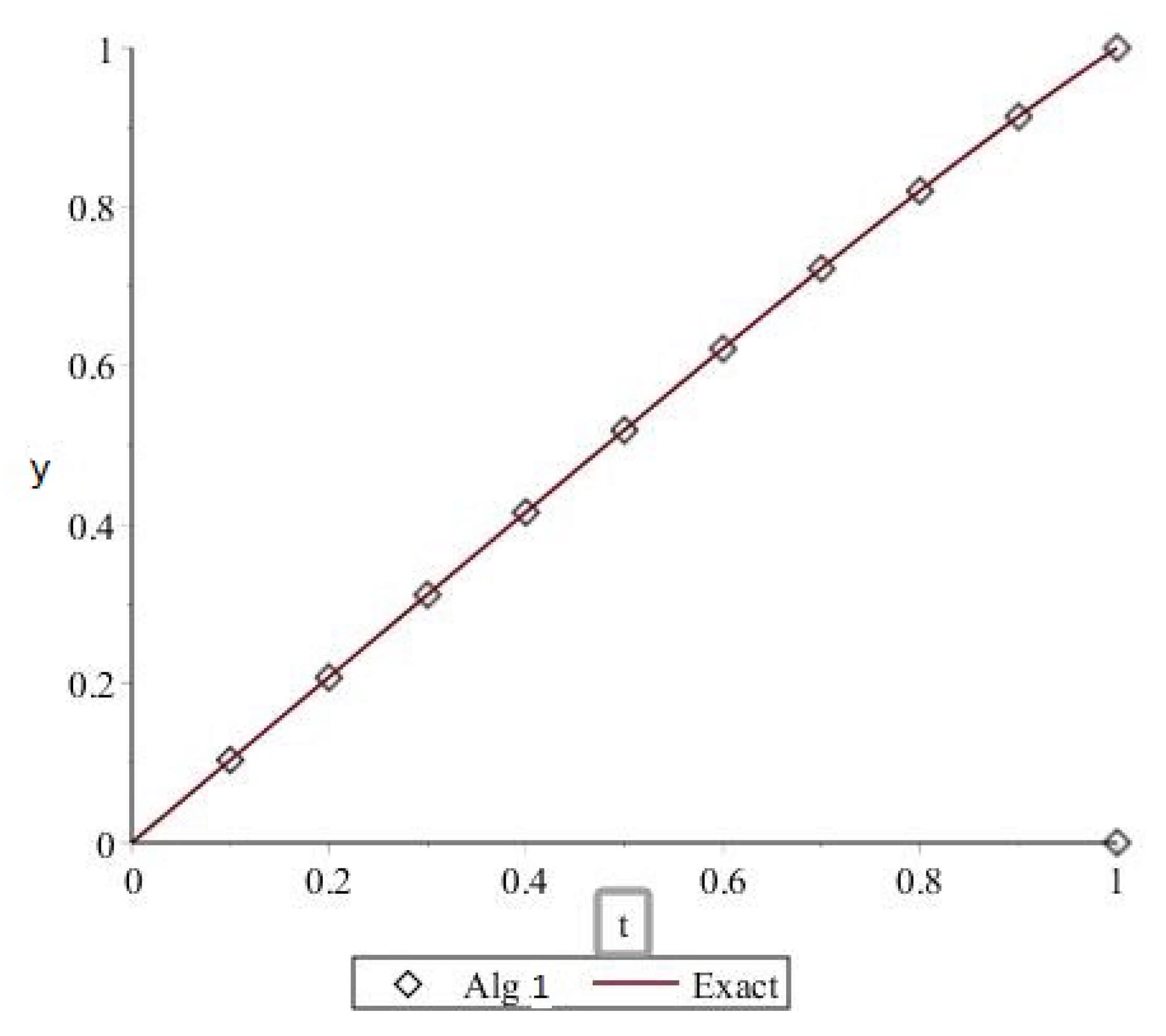
4. Numerical Results

In this section, we consider some problems to show the performance and efficiency of the newly developed method. We compare Newton’s method (NM) (see [6]) and methods (4), (5), (23), (25) and (27) in [15] with Algorithm 1. The stopping criterion is

$$Error=\left|\right|S^{(k+1)}-S^{\left(k\right)}{\left|\right|}_{\infty }<{10}^{-15},$$

and k denotes the number of iterations. The computational order of convergence q (see [16]) is approximated by

$$q\approx \frac{ln\left(\right||S^{(k+1)}-S^{\left(k\right)}||/|\left|S^{\left(k\right)}-S^{(k-1)}\left|\right|\right)}{ln\left(\left|\right|S^{\left(k\right)}-S^{(k-1)}\left|\right|/\left|\right|S^{(k-1)}-S^{(k-2)}\left|\right|\right)}.$$

(34)

Consider the following systems of nonlinear equations (see [16]).

Problem 1.

$\begin{array}{r}-x^2+{\displaystyle \frac{y^2}{6}}+y-17=0,\\ x^2-y-19=0,\end{array}$

Problem 2.

$\begin{array}{r}{x}^2+y^2+z^2-1=0,\\ 2x^2+y^2-4z=0,\\ 3x^2-4y^2+z^2=0.\end{array}$

Problem 3.

$\begin{array}{r}{e}^{x^2}+8xsin\left(y\right)=0,\\ x+2y-1=0.\end{array}$

Problem 4.

$\begin{array}{r}cos\left(x\right)-sin\left(y\right)=0,\\ z^x+1/y=0,\\ e^x-z^2=0.\end{array}$

Problem 5.

$\begin{array}{r}{x}^2+y^2+z^2-9=0,\\ xyz=1,\\ x+y-z^2=0.\end{array}$

Problem 6.

$\begin{array}{r}xy+xz+yz-1=0,\\ yz+w(y+z)=0,\\ xz+w(x+z)=0,\\ xy+w(x+y)=0.\end{array}$

Numerical results are given in Table 1 below.

Table 1. Numerical results for the Problems 1 to 6.

Method	Initial Guess	k	Approximate Solution	q
Problem 1
NM	${(5.5,6.8)}^T$	6	${(5.0000000000000,6.0000000000000)}^T$	2.0
(4)		4	${(5.0000000000000,6.0000000000000)}^T$	2.9
(5)		4	${(5.0000000000000,6.0000000000000)}^T$	2.9
(23)		4	${(5.0000000000000,6.0000000000000)}^T$	3.9
(25)		4	${(5.0000000000000,6.0000000000000)}^T$	3.9
(27)		4	${(5.0000000000000,6.0000000000000)}^T$	3.9
Algorithm 1		3	${(5.0000000000000,6.0000000000000)}^T$	5.9
Problem 2
NM	${(0.5,0.5,0.5)}^T$	6	${(0.698288610,0.628524230,0.342564189)}^T$	2.0
(4)		4	${(0.698288610,0.628524230,0.342564189)}^T$	3.0
(5)			${(0.698288610,0.628524230,0.342564189)}^T$	3.0
(23)		4	${(0.698288610,0.628524230,0.342564189)}^T$	4.0
(25)		4	${(0.698288610,0.628524230,0.342564189)}^T$	4.0
(27)		4	${(0.698288610,0.628524230,0.342564189)}^T$	4.0
Algorithm 1		3	${(0.698288610,0.628524230,0.342564189)}^T$	5.9
Problem 3
NM	${(0.5,1.0)}^T$	7	${(-0.22850805121143,0.61425402560572)}^T$	2.0
(4)		4	${(-0.22850805121143,0.61425402560572)}^T$	3.0
(5)		4	${(-0.22850805121143,0.61425402560572)}^T$	3.0
(23)		4	${(-0.22850805121143,0.61425402560572)}^T$	3.8
(25)		4	${(-0.22850805121143,0.61425402560572)}^T$	4.2
(27)		4	${(-0.22850805121143,0.61425402560572)}^T$	4.2
Algorithm 1		3	${(-0.22850805121143,0.61425402560572)}^T$	6.1
Problem 4
NM	${(1.0,0.5,1.5)}^T$	7	${(0.90956949,0.66122683,1.57583414)}^T$	2.0
(4)		5	${(0.90956949,0.66122683,1.57583414)}^T$	3.0
(5)		5	${(0.90956949,0.66122683,1.57583414)}^T$	3.0
(23)		4	${(0.90956949,0.66122683,1.57583414)}^T$	4.7
(25)		4	${(0.90956949,0.66122683,1.57583414)}^T$	4.1
(27)		4	${(0.90956949,0.66122683,1.57583414)}^T$	4.1
Algorithm 1		3	${(0.90956949,0.66122683,1.57583414)}^T$	6.3
Problem 5
NM	${(2.5,0.5,1.5)}^T$	7	${(2.49137571,0.2427458788,1.653517941)}^T$	2.0
(4)		5	${(2.49137571,0.2427458788,1.653517941)}^T$	3.0
(5)		5	${(2.49137571,0.2427458788,1.653517941)}^T$	3.0
(23)		4	${(2.49137571,0.2427458788,1.653517941)}^T$	4.5
(25)		4	${(2.49137571,0.2427458788,1.653517941)}^T$	4.5
(27)		4	${(2.49137571,0.2427458788,1.653517941)}^T$	4.5
Algorithm 1		3	${(2.49137571,0.2427458788,1.653517941)}^T$	6.1
Problem 6
NM	${(0.6,0.6,0.6,-0.2)}^T$	5	$(0.577350,0.577350,0.577350,{-0.288680)}^T$	2.1
(4)		4	$(0.577350,0.577350,0.577350,$−${0.288680)}^T$	3.3
(5)		4	$(0.577350,0.577350,0.577350,$−${0.288680)}^T$	3.3
(23)		3	$(0.577350,0.577359,0.577350,$−${0.288680)}^T$	5.5
(25)		3	$(0.577350,0.577350,0.577350,$−${0.288680)}^T$	5.5
(27)		3	$(0.577350,0.577350,0.577350,$−${0.288680)}^T$	5.5
Algorithm 1		3	$(0.577350,0.577350,0.577350,$−${0.288680)}^T$	6.0

Problem 7

([15]). Consider a nonlinear boundary-value problem of the following form:

$$\begin{array}{c}\hfill \begin{array}{cc}\hfill y^{″}\left(t\right)+y^{1+b}\left(t\right)& =0(t\in [0,1];b>0)\hfill \\ \hfill y\left(0\right)& =0,y\left(1\right)=1.\hfill \end{array}\end{array}$$

(35)

Here we have discretized the above nonlinear ODE (35) by using the finite difference method.

By taking $b=2.5$ and $n=10$, we obtain the following system of nonlinear equations.

$$\begin{array}{c}\hfill \begin{array}{cc}\hfill 100y_2-200y_1+y_1^{3.5}& =0,\hfill \\ \hfill 100y_3-200y_2+100y_1+y_2^{3.5}& =0,\hfill \\ \hfill 100y_4-200y_3+100y_2+y_3^{3.5}& =0,\hfill \\ \hfill 100y_5-200y_4+100y_3+y_4^{3.5}& =0,\hfill \\ \hfill 100y_6-200y_5+100y_4+y_5^{3.5}& =0,\hfill \\ \hfill 100y_7-200y_6+100y_5+y_6^{3.5}& =0,\hfill \\ \hfill 100y_8-200y_7+100y_6+y_7^{3.5}& =0,\hfill \\ \hfill 100y_9-200y_8+100y_7+y_8^{3.5}& =0,\hfill \\ \hfill -200y_9+100y_8+100+y_9^{3.5}& =0,\hfill \end{array}\end{array}$$

(36)

where $y^{\left(0\right)}={(1,1,1,1,1,1,1,1,1)}^T$ is the initial guess. We obtain the approximate solution as follows:

$$\begin{array}{cc}\hfill y^{*}=& (0.1039574502033\cdots ,0.2079117381290\cdots ,0.3118302489670\cdots ,\hfill \\ \hfill & 0.4156008747144\cdots ,0.5189667289214\cdots ,0.6214486996519\cdots ,\hfill \\ \hfill & {0.7222575415768\cdots ,0.8201966396108\cdots ,0.9135562704267\cdots )}^T.\hfill \end{array}$$

(37)

We compare Algorithm 1 with the Newton–Simpson method (NS-M) and the Open Newton method (ON-M) (see [9]), the four-point method (KH-M) (see [13]), the Newton–Gauss method (NG-M), and the fifth-order scheme (M 14) (see [15]). The numerical results are shown in Table 2 below.

Table 2. Numerical results for Problem 7.

Method	k	1	2	3	4	5
NS-M	$\left|\right|S_{k+1}-S_k{\left|\right|}_2$ q $\left|\right|F\left(S_k\right){\left|\right|}_2$	1.61121 3.20022 $4.3531\times {10}^{-3}$	$4.7021\times {10}^{-2}$ 2.98531 $5.6034\times {10}^{-8}$	$5.7614\times {10}^{-7}$ 2.99899 $1.2677\times {10}^{-22}$	$1.2500\times {10}^{-21}$ 2.99999 $1.3581\times {10}^{-66}$	$1.3253\times {10}^{-65}$ 3.00000 $1.6345\times {10}^{-198}$
ON-M	$\left|\right|S_{k+1}-S_k{\left|\right|}_2$ q $\left|\right|F\left(S_k\right){\left|\right|}_2$	1.61111 3.19700 $4.3121\times {10}^{-3}$	$46671\times {10}^{-2}$ 2.98555 $5.4934\times {10}^{-8}$	$5.6464\times {10}^{-7}$ 2.99891 $1.1944\times {10}^{-22}$	$1.17711\times {10}^{-21}$ 2.99999 $1.13333\times {10}^{-66}$	$1.10665\times {10}^{-65}$ 3.00000 $9.4989\times {10}^{-199}$
KH-M	$\left|\right|S_{k+1}-S_k{\left|\right|}_2$ q $\left|\right|F\left(S_k\right){\left|\right|}_2$	1 .61111 3.19921 $4.3411\times {10}^{-3}$	$4.6911\times {10}^{-2}$ 2.98555 $5.5731\times {10}^{-8}$	$5.7277\times {10}^{-7}$ 2.99800 $1.2455\times {10}^{-22}$	$1.2288\times {10}^{-21}$ 2.99999 $1.2888\times {10}^{-66}$	$1.2577\times {10}^{-65}$ 3.00000 $1.3951\times {10}^{-198}$
NG-M	$\left|\right|S_{k+1}-S_k{\left|\right|}_2$ q $\left|\right|F\left(S_k\right){\left|\right|}_2$	6.44555 3.19711 $4.3175\times {10}^{-3}$	$1.8681\times {10}^{-1}$ 2.98555 $5.5051\times {10}^{-8}$	$2.2633\times {10}^{-6}$ 2.99899 $1.2011\times {10}^{-22}$	$4.7391\times {10}^{-21}$ 2.99999 $1.1544\times {10}^{-66}$	$4.5099\times {10}^{-65}$ 3.00000 $1.0044\times {10}^{-198}$
M(14)	$\left|\right|S_{k+1}-S_k{\left|\right|}_2$ q $\left|\right|F\left(S_k\right){\left|\right|}_2$	1.64888 5.10032 $1.9300\times {10}^{-4}$	$2.0166\times {10}^{-3}$ 4.99732 $2.8741\times {10}^{-19}$	$2.8188\times {10}^{-18}$ 4.99999 $1.6941\times {10}^{-93}$	$1.6500\times {10}^{-92}$ 5.00000 $1.1788\times {10}^{-464}$	$1.1465\times {10}^{-463}$ 5.00000 $1.9077\times {10}^{-2320}$
Alg. 1	$\left|\right|S_{k+1}-S_k{\left|\right|}_2$ q $\left|\right|F\left(S_k\right){\left|\right|}_2$	$0.1622\times {10}^{-48}$ 6.10040 $0.7544\times {10}^{-47}$	0 6 0	- - -	- - -	- - -

From Table 2, we see that the proposed method converges to the solution in just two iterations. To illustrate the performance of the new method, we plot the approximate solution against the Maple solution in Figure 1.

Figure 1. Comparison between the exact solution ( Maple solution) and the approximate solution.

In the next problem, we compare Algorithm 1 with M6 [17] of order 6.

Problem 8.

Consider the following integral equation:

$$y\left(r\right)-1-\frac{y\left(r\right)}{4}\mu y\left(r\right){\int }_0^{1}k(r,u)y\left(u\right)du=0.$$

(38)

Solving (38), we have the following system of nonlinear equations:

$$y_i\approx 1+\frac{1}{8}{y}_i\sum _{j=1}^8\frac{u_i{\beta }_j}{u_i+u_j}{y}_j,i=1,2...8.$$

(39)

For more detail see [17]. We compare Algorithm 1 with M6 [17] in Table 3.

Table 3. Numerical results and comparison for Problem 8.

Method	Number of Iterations	Error
Newton	5	$3.1408\times {10}^{-16}$
M6	3	$2.2204\times {10}^{-16}$
Algorithm 1	3	$1.0000\times {10}^{-19}$

From the last column of Table 3, we conclude that the new method is more accurate than M6 [17].

5. Conclusions

In this article, we have implemented a new three-step Newton method for solving a system of nonlinear equations. The order of convergence of the proposed method is six. To show the effectiveness of the new method, we have provided some numerical tests. The graphical illustration shows the accuracy of the proposed method. Numerical results confirmed that the suggested method converges to the solution in fewer iterations with high accuracy, which justifies the advantage of this method.

References

1. Atkinson, K.E. An Introduction to Numerical Analysis, 2nd ed.; John Wiley and Sons: New York, NY, USA, 1987. [Google Scholar]
2. Abbasbandy, S. Extended Newton’s method for a system of nonlinear equations by modified Adomian decomposition method. Appl. Math. Comput. 2005, 170, 648–656. [Google Scholar] [CrossRef]
3. Babajee, D.K.R.; Dauhoo, M.Z. An analysis of the properties of the variants of Newton’s method with third order convergence. Appl. Math. Comput. 2006, 183, 659–684. [Google Scholar] [CrossRef]
4. Babajee, D.K.R.; Dauhoo, M.Z.; Darvishi, M.T.; Barati, A. A note on the local convergence of iterative methods based on Adomian decomposition method and 3-node quadrature rule. Appl. Math. Comput. 2008, 200, 452–458. [Google Scholar] [CrossRef]
5. Babolian, E.; Biazar, J.; Vahidi, A.R. Solution of a system of nonlinear equations by Adomian decomposition method. Appl. Math. Comput. 2004, 150, 847–854. [Google Scholar] [CrossRef]
6. Burden, R.L.; Faires, J.D. Numerical Analysis, 7th ed.; PWS Publishing Company: Boston, MA, USA, 2001. [Google Scholar]
7. Candelario, G.; Cordero, A.; Torregrosa, J.R. Multipoint Fractional Iterative Methods with (2α+1)th-Order of Convergence for Solving Nonlinear Problems. Mathematics 2020, 8, 452. [Google Scholar] [CrossRef] [Green Version]
8. Cordero, A.; Torregrosa, J.R. Variants of Newton’s method for functions of several variables. Appl. Math. Comput. 2006, 183, 199–208. [Google Scholar] [CrossRef]
9. Cordero, A.; Torregrosa, J.R. Variants of Newton’s method using fifth-order quadrature formulas. Appl. Math. Comput.. 2007, 190, 686–698. [Google Scholar] [CrossRef]
10. Darvishi, M.T.; Barati, A. A third-order Newton-type method to solve systems of nonlinear equations. Appl. Math. Comput. 2007, 187, 630–635. [Google Scholar] [CrossRef]
11. Darvishi, M.T.; Barati, A. Super cubic iterative methods to solve systems of nonlinear equations. Appl. Math. Comput. 2007, 188, 1678–1685. [Google Scholar] [CrossRef]
12. Darvishi, M.T.; Barati, A. A fourth-order method from quadrature formulae to solve system of nonlinear equations. Appl. Math. Comput. 2007, 188, 257–261. [Google Scholar] [CrossRef]
13. Khirallah, M.Q.; Hafiz, M.A. Novel three order methods for solving a system of nonlinear equations. Bull. Math. Sci. Appl. 2012, 2, 1–14. [Google Scholar] [CrossRef]
14. Noeiaghdam, S.; Araghi, M.A.F. A novel algorithm to evaluate definite integrals by the Gauss-Legendre integration rule based on the stochastic arithmetic: Application in the model of osmosis system. Math. Model. Eng. Prob. 2020, 7, 577–586. [Google Scholar]
15. Su, Q.-F. A unified model for solving a system of nonlinear equations. Appl. Math. Comput. 2016, 290, 46–55. [Google Scholar] [CrossRef]
16. Liu, Z.-L.; Zheng, Q.; Huag, C.-E. Third- and fifth-order Newton-Guass methods for solving system of nonlinear equations with n variables. Appl. Math. Comput. 2016, 290, 250–257. [Google Scholar]
17. Maduh, K. Sixth order Newton-Type method for solving system Of nonlinear equations and its applications. Appl. Math. E-Notes 2017, 17, 221–230. [Google Scholar]