An Efficient Shortest Path Algorithm: Multi-Destinations in an Indoor Environment

Abstract

The shortest path-searching with the minimal weight for multiple destinations is a crucial need in an indoor applications, especially in supermarkets, warehouses, libraries, etc. However, when it is used for multiple item searches, its weight becomes higher as it searches only the shortest path between the single sources to each destination item separately. If the conventional Dijkstra algorithm is modified to multi-destination mode then the weight is decreased, but the output path is not considered as the real shortest path among multiple destinations items. Our proposed algorithm is more efficient for finding the shortest path among multiple destination items with minimum weight, compared to the single source single destination and modified multi-destinations of Dijkstra’s algorithm. In this research, our proposed method has been validated by real-world data as well as by simulated random solutions. Our advancement is more applicable in indoor environment applications based on multiple items or destinations searching.

1. Introduction

In computer science, finding the shortest path in the complex indoor environment is a fundamental issue [1]. The solution to this issue is to use a bi-directional graph or road network to find the path with the minimal summation of edge weights among all reachable paths from start to end nodes [2]. The bi-directional graph considered in this paper is either directed or undirected, finite, simple, as well as connected [3]. The definition of a single pair shortest path is a path that contains only one destination. In conventional problems, the distances among the nodes are ascertained. The goal of the conventional single-source SPP is to get the minimal cost path from the source node to the destination node. However, the fuzzy number technique can be utilized instead in precarious environments [4]. The problem arises when the graph contains more than one destination node [5]. The set of destination nodes is a subset of all network nodes and it becomes a multi-destination shortest path problem [6], which has many real-life applications, such as finding the shortest path among multi-destination items in supermarkets, warehouses, libraries, road networks [7], robotics industries [8], service compositions [9,10], and multicast routes [11]. The different techniques found in the literature are calculating either a multi-destination or single-pair shortest path to solve these issues [12]. A* is an ordinary BFS algorithm that depends on a heuristic function to demonstrate the search towards finding the shortest path from a source node to a destination node in a grid [13]. As of now, Dijkstra’s is a renowned path searching algorithm that is mainly used for searching the shortest path from a single source to a single destination introduced by Edsger W. Dijkstra in 1956. A typical single-source single-destination, Dijkstra’s algorithm, is used for single-pair shortest path problems [14]. It keeps up a set S of unraveled nodes, consisting of those hubs or nodes whose ultimate shortest path between the starting node verses has ascertained as well as labels t(i), conserving the upward bound of the smallest pathway distance among v_s and v_i [15]. The node v_m ∈ V/S with the minimal t(i) is continually chosen by the algorithm, adding v_m to S, as well as updating t(i) as the node v_m [16]:

In the first step. Set t(v_s) = 0 and t(v_j) = w_sj.

For other nodes S = {v_s}, L = V/S

In the second step.

Chose a hub v_m from L, t(v_m) = $mi{n}_{v_{\mathrm{j}}\in L}t\left(v_{\mathrm{j}}\right)$,

if t(v_m) = 1, then stop, else move to third step.

In the third step set.

S = S U{v_m}, L = L\{v_m}

if L = ø, then stop, else move to forth step.

In the fourth step.

For each v_j ∈ L, update

t(v_j) = min{t(v_j),t(v_m) + w_mj

(1)

Move to first step.

In the above steps, V = {v_1, v₁, …, v_n} is the set of nodes, S is the set of the source nodes, L is a list, and W = w_ij is the weight matrix. The above steps demonstrate the shortest path calculation following the steps of Dijkstra’s algorithm and the final output is expressed in Equation (1).

The Modified Dijkstra’s Multi-Source Multi-Destination (MDMSMD) algorithm is applied for the multi-destination shortest path problem [17]. For the single-source multi-destination problem, the conventional Dijkstra’s single-source single-destination (CDSSSD) algorithm can be used. Although, in this network, the starting point is one node and destinations are a set of multiple nodes as a source node (s) and multiple destination nodes (w, x, y, z) as shown in Figure 1. As a result, it is necessary to calculate the shortest path between s to w, s to x, s to y, and s to z.

Figure 1. Bi-directional road network.

From the sample road network Figure 1, the steps of CDSSSD in Figure 2 is displayed. Figure 2a is the first step that calculates the shortest path between s and w from all accessible paths. Figure 2b is the second step that calculates the shortest path between s and x. Figure 2c shows the third step that calculates the shortest path between s and y, Figure 2d also shows the shortest path between x and z. In Figure 2e, all the calculated shortest paths among s and the destination nodes w, x, y, and z [18]. Here, the possible number of shortest paths is four. However, the number of paths can be converted to a single path from a source to the last destination node of a set of destination nodes by applying the MDMSMD. For example, a source node is s and the destination nodes are w, x, y, and z as per Figure 1. Hence, the shortest paths are between s and w, s and x, s and y, and s and z. The path of MDMSMD is s → w → x → y → z and has been expressed in Figure 3. In Figure 3a–e are respectively shown the shortest path between s → w is 10, w → x is 9, x → y is 11, y → z is 8 and s → w → x → y → z is 38. The minimum summation of edge weights of MDMSMD is less than CDSSSD. The MDMSMD solved the multi-destination path problem, with some limitations [19]. The MDMSMD calculates the shortest path from each source to each destination node, the previous destination node is the next source node, and calculates the shortest path from the next source to the next destination node until the last destination node. This algorithm can only calculate the shortest path between one pair at a time [20], it cannot calculate the shortest path between a source node and a set of destination nodes at the same time.

Figure 2. CDSSSD.

Figure 3. MDMSMD.

The objective of this research is to develop an efficient algorithm for searching the smallest path between a given source and the multi-destination nodes. The name of this proposed algorithm is the efficient algorithm for multi-destination shortest path problem (EAMDSP)—it accentuates the searching area and enhances the algorithm performance. The new concept is based on considering the outcome of the edge weights of the input graph on searching speed to acquire the goal. Using this concept, the EAMDSP finds the nearest destination node among the multiple destination nodes from the source node. After getting the first nearest destination node, it becomes the next source node and again calculates the next nearest destination node among the remaining multiple destination nodes until the last or rest destination node. Finally, the shortest path between a source node and the last destination node that decreases the summation of weights is achieved, which enhances the speed of searching for the desired shortest path. The proposed algorithm acquires the benefits of simplicity as well as the effectiveness of the computations. The outcomes of this algorithm using a real dataset and the simulated random solution will show that the proposed algorithm is better than the existing algorithm.

In this article, the following aims are discussed: Section 2, for the multi-destination shortest path problem, the existing method and solution have been reviewed as well as discussed. We propose an algorithm for searching the multi-destination shortest path in indoor environments in Section 3. In Section 4, the performance of the proposed algorithm is compared to the existing method and the conclusion is in Section 5.

2. Related Work

Nowadays, many researchers are working on graphical solutions and pathfinding to resolve crucial application issues [21,22,23,24,25,26,27]. Dijkstra’s algorithm is used for finding the solution to the shortest path problem in multi-destination nodes [28]. The Fibonacci heap [29,30] has been utilized in the multi-destination Dijkstra’s algorithm and is considered an innovative improvement. Searching the shortest paths by the node combination method is introduced by Lu et al. [31] by continually integrating with the source node’s contiguous neighbors. However, multi-destination Dijkstra’s algorithm is faster than their method. A quicker strategy with a small number of positive integer weights is introduced by Orlin et al. [32]. Thorup [33,34] invents an effective algorithm to solve the limitation of the Orlin et al. method which is an integral edge weight in every direction, as well as an undirected graph. In reality, no method has been utilized as an input of both undirected and directed graphs [35]. The breadth-first search, as well as the Bellman-Ford algorithm, are proposed respectively in the literature, while the graph contains all equal edge positive/negative weights. Searching the shortest path via a topological sequence [16] in linear time is feasible for a directed graph. An algorithm is introduced by Xu et al. [36] to effectively give a solution to the issue, particularly for infrequent networks.

In an article by [37], calculating the path as a usual job, so for every application [38,39] accelerate procedures perform based on the kind of data. A multi-destination feature of Dijkstra’s algorithm is becoming compatible with recent applications [40,41]. By utilizing an amended version of multiple destinations, Dijkstra’s algorithm is able to solve the bi-objective multi-destination shortest path problem in the pathway network which is introduced by Ticha et al. [7]. Their searching technique at each repetition of a process is to choose some parts of the path for a non-dominated path to arrive at one of the destination nodes. In the field of time schedule networks, Jin et al. [42] modified the multi-destination method for searching for the shortest path. First, they developed a path calculation method, then added it to the modified algorithm. Mainly, the shortest path calculation depends on the network constraints on its edges. By considering both node weights and edge weights, the multi-destination Dijkstra’s method enhancement is proposed by Ananta et al. [43]. For the software-defined networks, this method transmits data packets to all destination nodes. The limitations of multi-destination Dijkstra’s algorithm have been discussed in Section 1. This section also discussed the related algorithms, but they have some limitations such as one is designed only for a directed graph or only works on positive edge weight and another contains both positive and negative edge weight. The proposed algorithm has been designed for removing their short-comings and can perform on a bi-directional graph or road network, as well as finding the shortest path from the starting node to the multiple destination nodes, as is required in indoor environments.

3. Algorithms

Algorithm 1 (CDSSSD) and Algorithm 2 (MDMSMD) are used as reference algorithms to compare the performance of our proposed Algorithm 3. The steps of CDSSSD, MDMSMD, and EAMDSP are provided in this section to demonstrate a clear overview.

3.1. Algorithm: CDSSSD

Algorithm 1 Input: Graph: G (V, E, W), source node: S, set of multiple destination nodes: T Output: Paths from source to destination nodes

Declare: L   For (i = 0; I < T.Length; i++)     Declare: nodes_path     n: = G.GetLength(0);     distance: = new int[n];     For (int k = 0; k < n; i++)      distance[i]: = int.MaxValue;     End For     distance[S]: = 0;     used: = new bool[n];     Previous: = new int?[n];     While (true)      minDistance: = int.MaxValue;      minNode: = 0;      For (int m = 0; m < n; m++)       If (!used[m] && minDistance > distance[m])        minDistance: = distance[m];        minNode: = m;       End If      End For      If (minDistance == int.MaxValue)       break;      End If      used[minNode]: = true;      For (int l = 0; l < n; l++)       If (G[minNode, l] > 0)        shortestToMinNode: = distance[minNode];        distanceToNextNode: = G[minNode, l];        totalDistance: = shortestToMinNode + distanceToNextNode;        If (totalDistance < distance[l])         distance[l]: = totalDistance;         previous[l]: = minNode;        End If       End If      End For     End While     If (distance[T[i]] :== int.MaxValue)      return null;     End If     currentNode: = T[i];     While (currentNode ! = null)      Add nodes_path->col: = currentNode.Value;      currentNode: = previous[currentNode.Value];     End While     col1: = S;     For(j = 0;j < nodes_path.Length;j++)      Add L->col: = nodes_path[j]      col1: = nodes_path[j];     End For   End For  Return L;

3.2. Algorithm: MDMSMD

Algorithm 2 Input: Graph: G (V, E, W), source node: S, set of multiple destination nodes: T Output: A path from source to destination nodes and shortest path among destination nodes

Declare: L   For (i = 0;I < T.Length;i++)     Declare: nodes_path     n: = G.GetLength(0);     distance: = new int[n];     For (int k = 0; k < n; i++)       distance[i]: = int.MaxValue;     End For     distance[S]: = 0;     used: = new bool[n];     Previous: = new int?[n];     While (true)       minDistance: = int.MaxValue;       minNode: = 0;       For (int m = 0; m < n; m++)         If (!used[m] && minDistance > distance[m])          minDistance: = distance[m];          minNode: = m;         End If       End For       If (minDistance == int.MaxValue)         break;       End If       used[minNode]: = true;       For (int l = 0; l < n; l++)        If (G[minNode, l] > 0)          shortestToMinNode: = distance[minNode];          distanceToNextNode: = G[minNode, l];          totalDistance: = shortestToMinNode + distanceToNextNode;          If (totalDistance < distance[l])           distance[l]: = totalDistance;           previous[l]: = minNode;          End If         End If       End For     End While     If (distance[T[i]] :== int.MaxValue)       return null;     End If     currentNode: = T[i];     While (currentNode ! = null)       Add nodes_path->col: = currentNode.Value;       currentNode: = previous[currentNode.Value];     End While     col1: = S;     For(j = 0;j < nodes_path.Length;j++)       Add L->col: = nodes_path[j]       col1: = nodes_path[j];     End For     S: = T[i];   End For   Return L;

3.3. The Proposed EAMDSP

In algorithm 3, we consider that G = (V, E, W) is a graph containing N nodes (vertices), a set of edges, and a set of weights. The vertex set V has n = |V| collection of nodes, E contains m = |E| and is the collection of edges, as well as W, the collection of weights.

Let _We ∈ W be the weight of edge e = (u, v) ∈ E as u → v for some u, v ∈ V.

The objective is to find a collection of shortest paths among vertices s ∈ V as an assigned origin node to the collection of multi-destination nodes d_i ∈ D ⊆ V, i ∈ I = {1, 2,..., |D|}. For instance, $w_{path\left(s, d_i\right)}$ = ${{\displaystyle \sum }}_j^{\left|path\left(s, d_i\right)\right|}{w}_{ej}$ where the path(s, d_i) is the weight of path and pd_i (i ∈ I) is the shortest path containing the minimal weight of $w_{path\left(s, d_i\right)}$ among all accessible paths from s to d_i. Here, if there is no path from s to d_i then δpd_i = ∞ else δpd_i = δpath(s,d_i) = min{w_path(s,di)}. Figure 1 explains the details of this scenario.

The proposed algorithm, EAMDSP, provides the shortest path from source node s ∈ V to all destination nodes or multi-destination nodes d_i ∈ T ⊆ V, i ∈ I in the graph G = (V, E, W).

Firstly, find the nearest destination node from the set of destination nodes by calculating the shortest path among all possible paths using Dijkstra’s single source-single destination algorithm.

Secondly, the nearest destination node from the source node is identified by minimum visited nodes and a minimum sum of weights between the source and each destination node.

Thirdly, after getting the first nearest destination node, it is considered as the next source node and starts the calculation of the nearest destination node from the rest of the destination nodes. This procedure is repeated until the last rest destination node. Getting the visited nodes from the source to the first nearest node combines the visited nodes, and goes for the next sources and continues until the last shortest path. The minimum sum of weights also adds as the above-visited nodes. Finally, the path that is found from the source to the last destination is the shortest path between the source to multi-destination nodes with minimum visited nodes and the minimal sum of weights.

For instance, in Figure 1, the source node is s and destination nodes are sequentially w, x, y, and z. In Figure 4, the steps of EAMDSP have been demonstrated in Figure 1, with a sample bi-directional road network with weights and nodes. In step (a) of Figure 4, the sum of weights calculated from s to w is 10, s to x is 9, s to y is 15, and s to z is 12, and are found after calculating the shortest path among possible accessible paths.

Figure 4. Graphical representation of EAMDSP.

First, each shortest path is s → x then x becomes the source node in the next step (b) of Figure 4. Similarly, the rest (w, y, z) are destination nodes, and again calculation on the sum of the weights from x to w is 9, x to y is 11, and x to z is 7. Secondly, the shortest path is x → z and combined with the minimum visited nodes between x → z. Furthermore, the previous minimum visited nodes between s > x are combined with the minimum sum of weights from s → x to x → z.

Now in step (c) of Figure 4, z is the source and w and y are destination nodes. Again, the calculation is done on the shortest path between z → y and z → w. The minimum sum of weights between z → y is eight and z → w is nine. the shortest path is z → y and combined with the minimum visited nodes between z > y. The previous minimum visited nodes between z > y are combined with the minimum sum of weights from s > x > z to z > y.

In step (d) of Figure 4, calculate the shortest path between y to w and get the sum of the weight values. Finally, the shortest path is s → x → z → y → w, and the total sum of weights is 33.

The MDMSMD working has been discussed in Section 1. The EAMDSP calculates the nearest destination node from the set of destination nodes that is the main difference from the MDMSMD. In the above example, the MDMSMD path will be s → w → x-y-z and the total sum of weight is 38. The CDSSSD total sum of weights is 46 from the above example. The number of total visited nodes and the sum of minimum weights of EAMDSP is less than the MDMSMD and the CDSSSD. As a result, EAMDSP is more efficient than MDMSMD and CDSSSD.

Algorithm 3. Raised algorithm: EAMDSP

Input: Graph: G (V, E, W), source node: S, set of multiple destination nodes: T  Output: A path from source to destination nodes and shortest path among destination nodes Declare: L1, L2, L3  While(T.Length>0)   For ( I = 0;I < T.Length;i++)     nodes_path: = singleSourceSingleDestinationAlgorithm(G,S,T[i])     For(j = 0;j < nodes_path.Length;j++)       length_path: = length_path + G[nodes_path [j], nodes_path[j + 1]]       Add L2->col1: = nodes_path[j], L2->col2: = T[i]     End For     Add L1->col1: = T[i], L1->col2: = length_path   End For   L1 sorting according to length_path   e_Dest_Node: = L1->col1   For (m = 0; m < L2.Length; m++)    IF L2[m]->col2== e_Dest_Node     Add L3->col: = L2[m]->col1    End IF   End For   S: = e_Dest_Node   Remove the e_Dest_Node value from T   L1: = new initialize   L2: = new initialize   End While   Return L3;

In the above algorithm, the variables L1 and L2 are declared as a two-dimensional array and L3 is a one-dimensional array for data storage. The first “while” loop runs until the last destination nodes come. The first “for” loop runs until the number of destination nodes are exhausted. The single-source single-destination algorithm is called to find the shortest path for visiting nodes among the source nodes to each destination node. The second “for” loop runs until the total number of shortest paths finding is completed for visiting nodes. Then the total path length or weight is calculated among the shortest path of visited nodes. Store each visited node into col1 of L2 and each destination node into col2 of L2. After that, store each destination node into col1 of L1 and path length or weight from a source to each destination node into col2 of L1. Sorting L1 according to path length or weight (smallest to biggest). Top each destination node from L1 → col1 first index (the smallest distance). Another new “for” loop is started for looping until L2 length or several destination nodes are covered. IF condition L2 [m]—>col2 == e_Dest_Node, then store the visiting nodes from a source to a destination in L3. S: = e_Dest_Node, replace current destination node value to source node value like the previous destination node is the next source node. Remove each destination node value from D. Then, L1: = new initialize or empty and L2: = new initialize or empty. Finally return L3, where L3 contains the source to all destination visiting nodes with the shortest path.

In Figure 5, $p{h}_u$ is the shortest path and $p^{\prime }{h}_u$ is an alternative path s → u via hubs i and j. S is a set (shady zone) of all hubs whose ultimate smallest pathway from the source s has been ascertained.

Figure 5. Source and destination shortest pathfinding in graphical representation.

Theorem 1.

(Exactness) The ultimate smallest path among destination nodes d_i ∈ D is constantly provided by EAMDSP, for example, d_i.t = δpath (s, sd_i), i ∈ I. The penultimate set T_i contains several nodes, which are linked to the destination node d_i.

Proof. 

For each u ∈ V and t ∈ T assuming the algorithm found the label u.t, as well as the smallest path’s weight, is δpath(s,u) for s → u. It aims to prove u.t = δpath(s,u) where each vertex u returned at the end of the EAMDSP. □

Initial case, s.t = δpath(s,s) = 0, when S = {s} for every v ∈ S which considers v.t shows the real smallest path’s weight among s and v,

v.t = δpath(s,v)

(2)

In this algorithm, −1 is used for u as a subsequent vertex to set S via path $p{h}_u$, therefore, u.t = $\delta p{h}_u$. It will prove this path to be the minimum distance,

u.t = δpath(s,u)

(3)

Assume the minimum distance s → u is the alternate path $p^{\prime }{h}_u$ instead of the path $p{h}_u$. The cost of the path $p{h}_u$ is more than the cost of the path $p^{\prime }{h}_u$

$$p{h}_u>p^{\prime }{h}_u=u.t$$

(4)

Equation (4) is explained in Figure 2, the path $p^{\prime }{h}_u$, begins in S as well as at a few points omits S to arrive at the node u that is as of now not in S. Assume (m, n) is the 1st edge toward $p^{\prime }{h}_u$ that departs from S. Evidently, $w_{path\left(s,m\right)}$ + $w_{path\left(m,n\right)}$ < ${\delta }_{p^{\prime }{h}_u}$. While m ∈ S, m.t is the cost of the minimum distance s → m path by the inductive hypothesis, m.t = ${\delta }_{path\left(s,m\right)}$ ≤ $w_{path\left(s,m\right)}$, which implies m.t + $w_{\left(m,n\right)}$ ≤ ${\delta }_{p^{\prime }{h}_u}$. The algorithm must update n.t while n is adjacent to m, which means n.t ≤ m.t + $w_{\left(m,n\right)}$. The u must have the shortest value due to the algorithm picked u, in other words, u.t ≤ n.t. To sum up these disparities, we present the outcomes in Section 4.

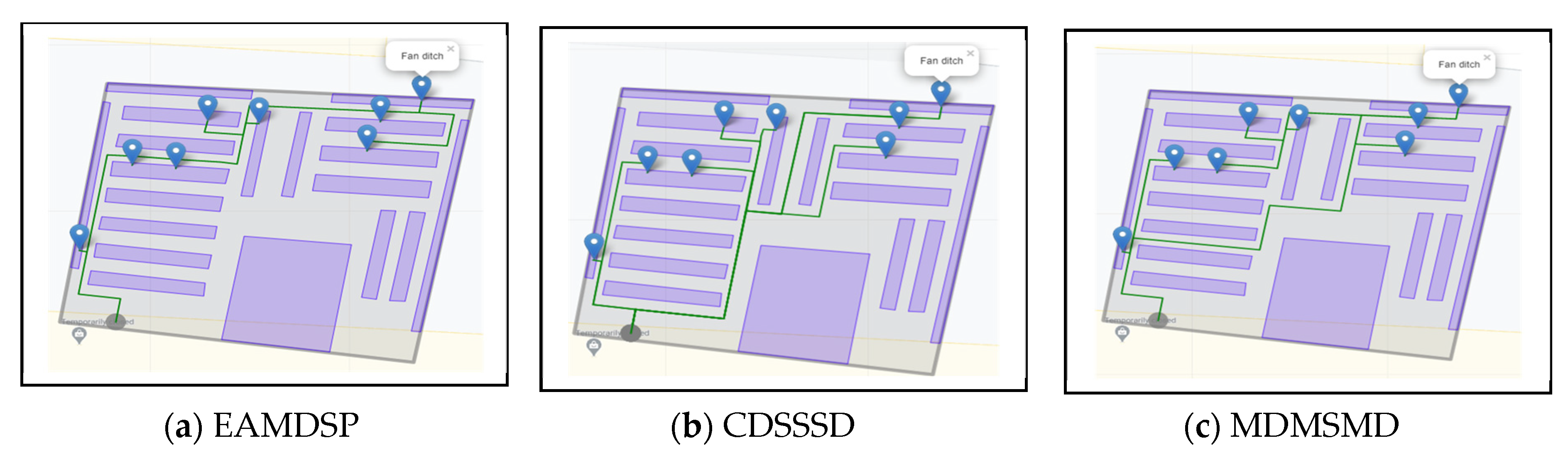
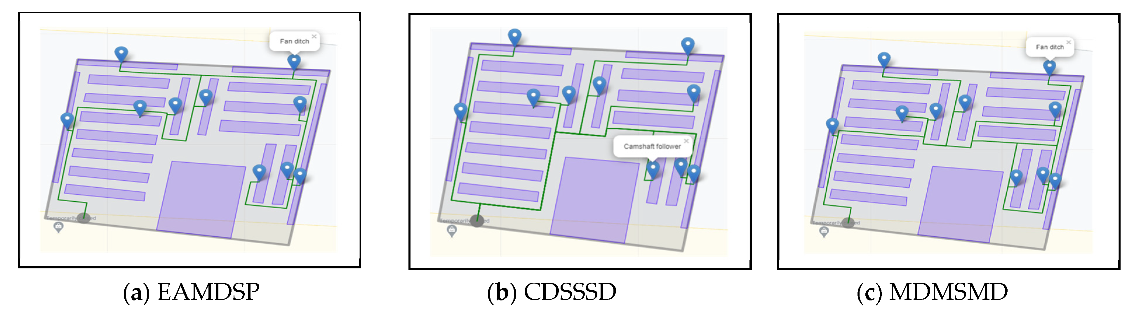
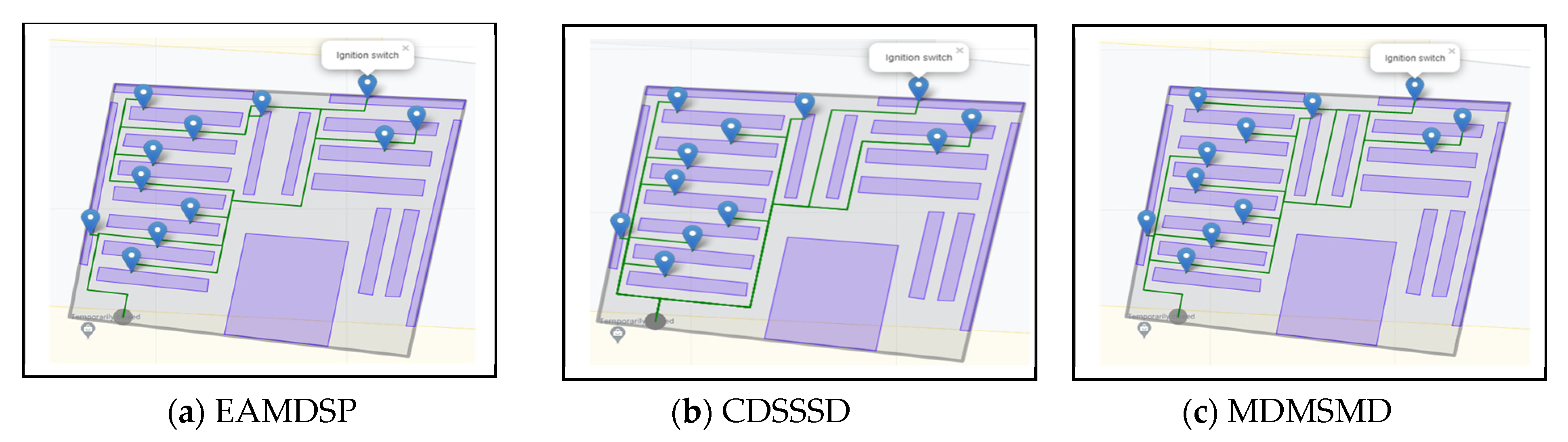
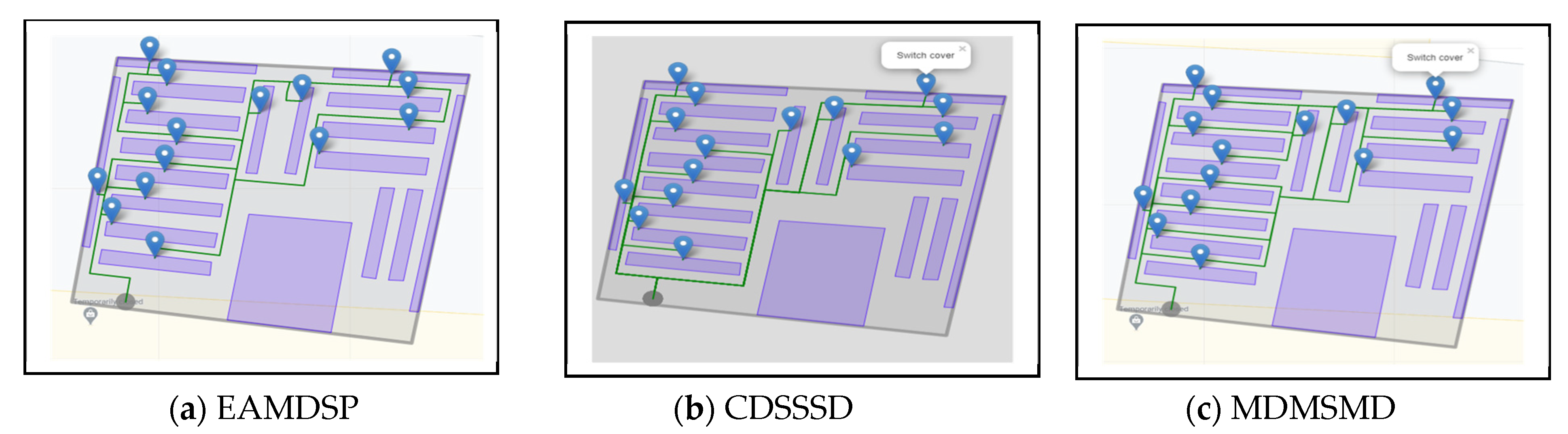
4. Results and Discussion

In this section, the detailed simulation results of EAMDSP, CDSSSD, and MDMSMD will be presented. To evaluate the proposed EAMDSP simulation performance CDSSSD and MDMSMD simulation results on the same layout were used. The performance was evaluated concerning the number of nodes visited and the weight or cost. Two different scenarios, one was the car spare parts shop and another was the supermarket used for getting the comprehensive results. In the car spare parts shop scenario, the simulations were run in six unique phases as in four, six, eight, ten, twelve, and fifteen items searching layout. Three shortest path algorithms named CDSSSD, MDMSMD, and EAMDSP were used on both scenarios in different phases for getting a different result. The results comparisons are showed in the layout simulation, the summary table, and the graph.

Figure 6 shows the layout of a spare parts shop containing shelves (nodes) and road networks. The road network also consists of nodes. Every node has a unique number with longitude and latitude. The road network’s one node is connected to the neighbor node with edge and weight value. The product/item is placed on the shelve node. The shelf node is connected to the road network’s node with an edge and the edge has a weight value. When searching for a product, the product’s shelf node number is considered to be the destination node. The shortest path was calculated between the source point (starting point) and the destination node, using the minimum the total nodes visited and their minimum weight or cost.

Figure 6. Drawing layout in a car spare part shop with nodes.

Table 1 represents the input which is the randomly selected four items. These input items were used for the same simulation layout of three algorithms such as CDSSSD, MDMSMD, and proposed EAMDSP.

Table 1. Selected four items and categories (input).

Item	Category
Antenna cable	Audio/video devices
Bumper	Body components, including trim
Adjusting mechanism	Braking system
Bucket seat	Car seat

Figure 7a–c are car spare parts shop simulation result of EAMDSP, CDSSSD and MDMSMD respectively, which show the shortest path among four items. Table 2 shows the output summary data for the four-item search. EAMDSP for the shortest path between the above four items visited 93 nodes and had a total weight of 95. However, using CDSSSD and MDMSMD for the same items, the visited nodes were 124 and 120 and the total cost was 136 and 125, respectively. Therefore, the proposed EAMDSP is efficient for visited nodes and total weight. Finally, total visited nodes or total cost can be expressed as EAMDSP < MDMSMD < CDSSSD. The detailed data for the four items are shown in Appendix A.

Figure 7. Simulation on a car spare parts shop scenario using EAMDSP, CDSSSD, and MDMSMD for a four-item search (output scenario).

Table 2. Summary data of EAMDSP, CDSSSD, and MDMSMD for a four-item search.

SL No.	Algorithm Name	Total Visited Nodes	Total Cost
1	EAMDSP	93	95
2	CDSSSD	124	136
3	MDMSMD	120	125

Table 3 represents the input value, which is six items randomly selected. These input items were used on the same simulation layout as the three algorithms CDSSSD, MDMSMD, and EAMDSP.

Table 3. (Input) Selecting six items and category.

Item	Category
Antenna assembly	Audio/video devices
ABS steel pin	Braking system
Back seat	Car seat
Door switch	Electrical switches
Distributor cap	Engine components and parts
Oil gasket	Engine oil systems

Figure 8a–c are car spare parts shop simulation result of EAMDSP, CDSSSD and MDMSMD, respectively which show the shortest path among six items. Table 4 shows the output summary data for the six-item search. EAMDSP for the shortest path between the six items visited 129 nodes and the total weight was 131. However, when using CDSSSD and MDMSMD for the same items, the visited nodes were 220 and 175 and the total cost was 242 and 179, respectively. Therefore, EAMDSP is efficient in terms of visited nodes and total weight. Finally, total visited nodes, or total cost can be expressed as EAMDSP < MDMSMD < CDSSSD.

Figure 8. Simulation on a car spare parts shop scenario using EAMDSP, CDSSSD, and MDMSMD for a six-item search (output scenario).

Table 4. Summary data of EAMDSP, CDSSSD, and MDMSMD for a six-item search.

SL No.	Algorithm Name	Total Visited Nodes	Total Cost
1	EAMDSP	129	131
2	CDSSSD	220	242
3	MDMSMD	175	179

Table 5 represents the input values of the eight items. These input items were used for the same simulation layout using three algorithms CDSSSD, MDMSMD, and EAMDSP.

Table 5. (Input) Selecting eight items and category.

Item	Category
Radio and media player	Audio/video devices
Cowl screen	Body components, including trim
Adjusting mechanism (adjuster star wheel)	Braking system
Dashcam	Cameras
Bench seat	Car seat
Central locking	Doors
Fan ditch	Electrical switches
Engine compartment harness	Wiring harnesses

Figure 9a–c are car spare parts shop simulation result of respectively EAMDSP, CDSSSD and MDMSMD which show the shortest path among eight items. Table 6 shows the output summary data for the eight items searched. When using EAMDSP for the shortest path between the above eight items, 119 nodes were visited, and the total weight or cost was 121. However, when using CDSSSD and MDMSMD for the same items, the visited nodes were 271 and 227 and the total cost was 297 and 239, respectively. So, EAMDSP is efficient for visited nodes and the total weight or cost. Finally, total visited nodes, or total cost can be expressed as EAMDSP < MDMSMD < CDSSSD.

Figure 9. Simulation on a car spare parts shop scenario using EAMDSP, CDSSSD, and MDMSMD for an eight-item search (output scenario).

Table 6. Summary data of EAMDSP, CDSSSD, and MDMSMD for an eight-item search.

SL No.	Algorithm Name	Total Visited Nodes	Total Cost
1	EAMDSP	119	121
2	CDSSSD	271	297
3	MDMSMD	227	239

Table 7 represents the input value of ten items. These input items were used for the same simulation layout of three algorithms CDSSSD, MDMSMD, and EAMDSP.

Table 7. (Input) Selecting ten items and category.

Item	Category
Radiator core support	Body components
Brake pad	Braking system
Fan ditch	Electrical switches
Camshaft follower	Engine components and parts
PCV valve	Engine components and parts
Oil suction filter	Engine oil systems
Battery box	Low voltage electrical supply system
Alarm and siren	Miscellaneous
Wiring connector	Miscellaneous
Glowplug	Starting system

Figure 10a–c are car spare parts shop simulation result of EAMDSP, CDSSSD and MDMSMD respectively, which show the shortest path among ten items. Table 8 shows the output summary data for the ten-item search. When using EAMDSP for the shortest path between the above 10 items, 164 nodes were visited and the total weight or cost was 170. However, when using CDSSSD and MDMSMD for the same items, the visited nodes were 377 and 227, and the total cost was 414 and 236, respectively. Therefore, EAMDSP is efficient for visited nodes and total weight or cost. Finally, total visited nodes, or total cost can be expressed as EAMDSP < MDMSMD < CDSSSD.

Figure 10. Simulation on a car spare parts shop scenario using EAMDSP, CDSSSD, and MDMSMD for a ten-item search (output scenario).

Table 8. Summary data of EAMDSP, CDSSSD, and MDMSMD for a ten-item search.

SL No.	Algorithm Name	Total Visited Nodes	Total Cost
1	EAMDSP	164	170
2	CDSSSD	377	414
3	MDMSMD	227	236

Table 9 represents the input value of twelve items. These input items were used for the same simulation layout of three algorithms CDSSSD, MDMSMD, and EAMDSP.

Table 9. (Input) Selecting twelve items and category.

Item	Category
Tuner	Audio/video devices
Fascia rear and support	Body components
Brake backing plate	Braking system
Front seat	Car seat
Front Right Outer door handle	Doors
Ignition switch	Electrical switches
Fuel gauge	Gauges and meters
Ignition magneto	Ignition system
Side lighting	Lighting and signaling system
Coolant temperature sensor	Sensors
Sunroof glass	Windows
Air conditioning harness	Wiring harnesses

Figure 11a–c are car spare parts shop simulation result of EAMDSP, CDSSSD and MDMSMD respectively, which show the shortest path among twelve items. Table 10 shows the output summary data for the twelve items searched. When using EAMDSP for the shortest path between the above twelve items, 213 nodes were visited and the total weight or cost was 220. However, when using CDSSSD and MDMSMD for the same items, the visited nodes were 378 and 315 and the total cost was 408 and 327, respectively. Therefore, EAMDSP is efficient for visited nodes and total weight or cost. Finally, total visited nodes, or total cost can be expressed as EAMDSP < MDMSMD < CDSSSD.

Figure 11. Simulation on a car spare parts shop scenario using EAMDSP, CDSSSD, and MDMSMD for a twelve-item search (output scenario).

Table 10. Summary data of EAMDSP, CDSSSD, and MDMSMD for a twelve-item search.

SL No.	Algorithm Name	Total Visited Nodes	Total Cost
1	EAMDSP	213	220
2	CDSSSD	378	408
3	MDMSMD	315	327

Table 11 represents the input values of the selected fifteen items. These input items were used for the same simulation layout of three algorithms CDSSSD, MDMSMD, and EAMDSP.

Table 11. (Input) Selecting fifteen items and categories.

Item	Category
Front fascia and header panel	Body components
Brake disc	Braking system
Brake booster hose	Braking system
Backup camera	Cameras
Headrest	Car seat
Rear left side outer door handle	Doors
Switch cover	Electrical switches
Odometer	Gauges and meters
Distributor	Ignition system
Engine bay lighting	Lighting and signaling system
Shift improver	Miscellaneous
Knock sensor	Sensors
Starter drive	Starting system
Front left side door glass	Windows
Floor harness	Wiring harnesses

Figure 12a–c are car spare parts shop simulation result of EAMDSP, CDSSSD and MDMSMD respectively, which show the shortest path among fifteen items. Table 12 shows the output summary data for the fifteen-item search. When using EAMDSP for the shortest path among the above fifteen items, 225 nodes were visited and the total weight or cost was 233. However, when using CDSSSD and MDMSMD for the same items, the visited nodes were 487 and 393 and the total cost was 525 and 409, respectively. Therefore, our proposed shortest path algorithm EAMDSP is efficient for visited nodes and total weight or cost. Finally, total visited nodes, or total cost can be expressed as EAMDSP < MDMSMD < CDSSSD.

Figure 12. Simulation on a car spare parts shop scenario using EAMDSP, CDSSSD, and MDMSMD for a fifteen-item search (output scenario).

Table 12. Summary data of EAMDSP, CDSSSD, and MDMSMD for a fifteen-item search.

SL No.	Algorithm Name	Total Visited Nodes	Total Cost
1	EAMDSP	225	233
2	CDSSSD	487	525
3	MDMSMD	393	409

Figure 13 shows the cost-wise comparison among EAMDSP, CDSSSD and MDMSMD as per Table 13.

Figure 13. Cost-wise comparison among EAMDSP, CDSSSD, and MDMSMD.

Table 13. Total cost-wise comparison among EAMDSP, CDSSSD, and MDMSMD.

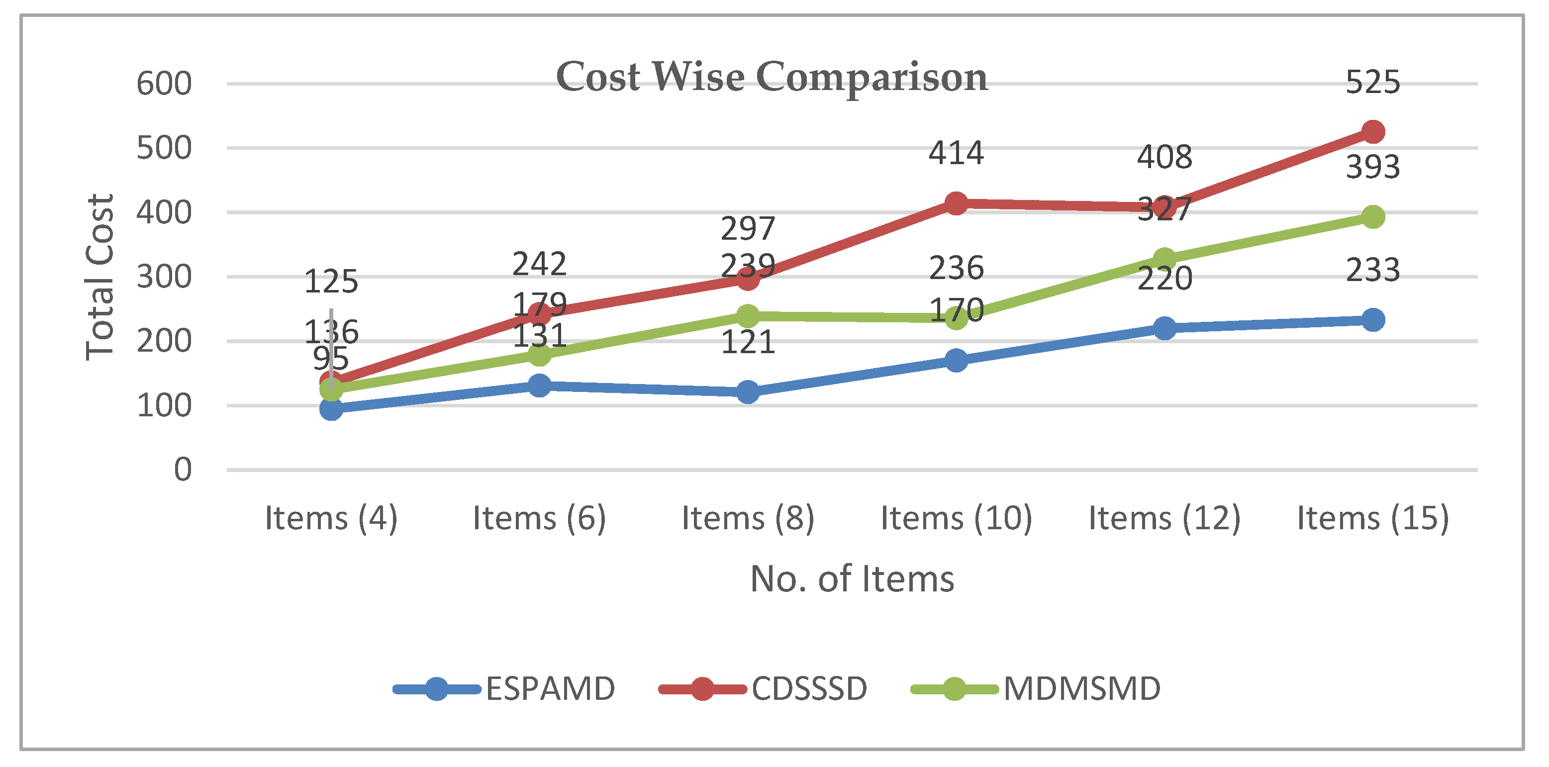
SL No.	Algorithm Name	Items (4)	Items (6)	Items (8)	Items (10)	Items (12)	Items (15)
1	EAMDSP	95	131	121	170	220	233
2	CDSSSD	136	242	297	414	408	525
3	MDMSMD	125	179	239	236	327	409

Figure 14 shows the visited-wise comparison among EAMDSP, CDSSSD and MDMSMD as per Table 14.

Figure 14. Visited nodes-wise comparison between EAMDSP, CDSSSD, and MDMSMD.

Table 14. Total visited node-wise comparison among EAMDSP, CDSSSD, and MDMSMD.

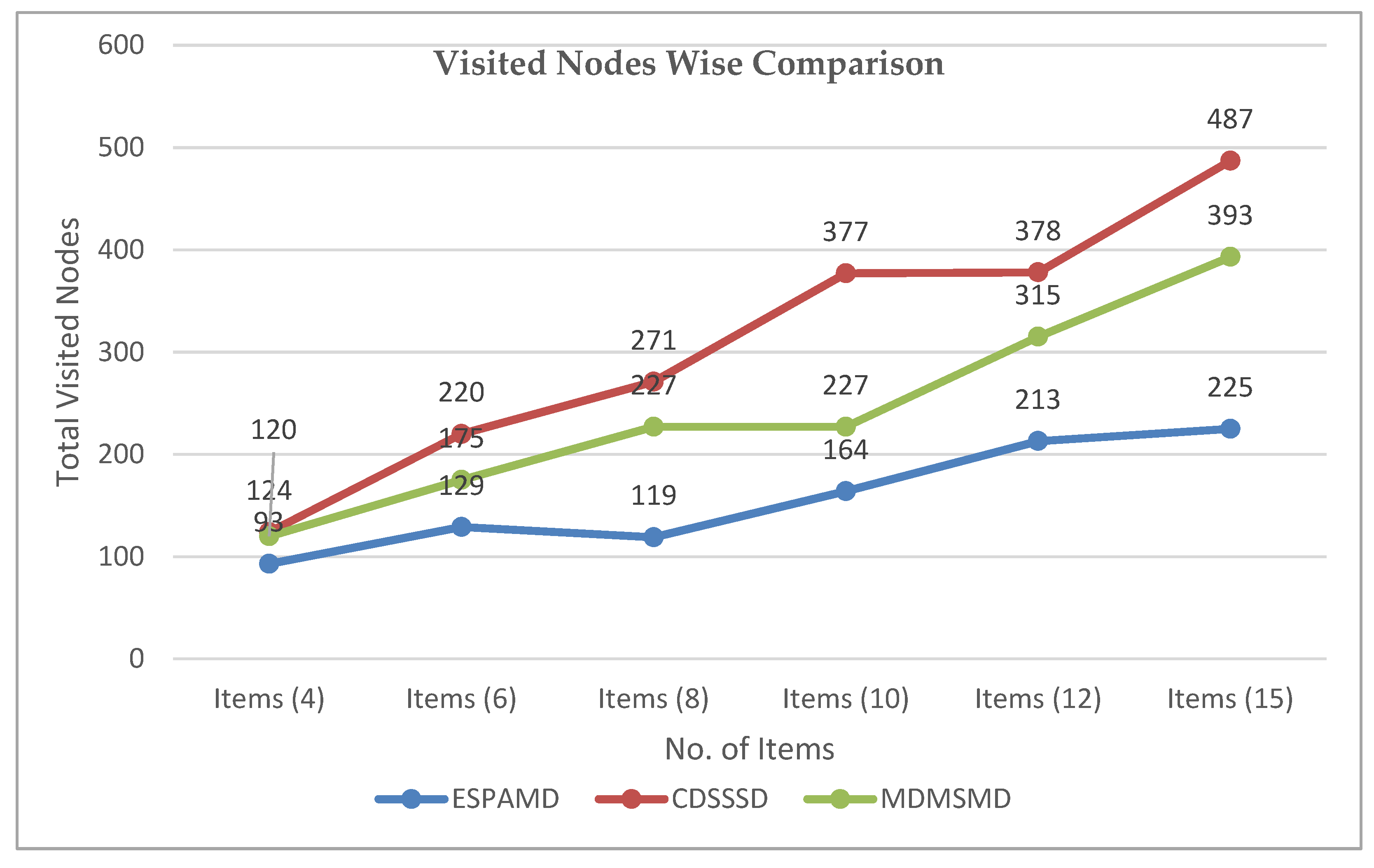
SL No.	Algorithm Name	Items (4)	Items (6)	Items (8)	Items (10)	Items (12)	Items (15)
1	EAMDSP	93	129	119	164	213	225
2	CDSSSD	124	220	271	377	378	487
3	MDMSMD	120	175	227	227	315	393

In Figure 15, we present another scenario similar to a supermarket simulation scenario, the simulations were run in three unique phases as a five, eight, and eleven-item searching layout. Three shortest path algorithms CDSSSD, MDMSMD, and our proposed EAMDSP were used in this scenario’s different phases for getting the different results and comparing results shown in the layout simulation. Summary data is presented in tables and graphs.

Figure 15. Drawing layout in the supermarket with nodes.

Table 15 represents the input value, which was randomly selected for five items. These input items were used for the same simulation layout of three algorithms CDSSSD, MDMSMD, and EAMDSP.

Table 15. (Input) Selecting five items and categories.

Item	Category
Coffee	Beverages
Dinner rolls	Bread/Bakery
Vegetables	Canned/Jarred goods
Laundry detergent	Cleaners
Yogurt	Dairy

Figure 16a–c are supermarket simulation result of respectively EAMDSP, CDSSSD and MDMSMD which show the shortest path among five items. Table 16 shows the output summary data for the five-item search. When using EAMDSP for the shortest path between the above the five items, 45 nodes were visited and the total weight was 54. However, when using CDSSSD and MDMSMD for the same items, the visited nodes were 60 and 52 and the total cost was 84 and 69, respectively. Therefore, our proposed shortest path algorithm EAMDSP is efficient for visited nodes and total cost. Finally, total visited nodes, or total cost can be expressed as EAMDSP < MDMSMD < CDSSSD.

Figure 16. Simulation on supermarket scenario using EAMDSP, CDSSSD, and MDMSMD for a five-item search (output scenario).

Table 16. The output summary data of EAMDSP, CDSSSD, and MDMSMD for a five-item search.

SL No.	Algorithm Name	Total Visited Nodes	Total Cost
1	EAMDSP	45	54
2	CDSSSD	60	84
3	MDMSMD	52	69

Table 17 represents the input values of the selected eight items. These input items were used for the same simulation layout of three algorithms CDSSSD, MDMSMD, and EAMDSP.

Table 17. (Input) Selecting eight items and categories.

Item	Category
Soda	Beverages
Sandwich loaves	Bread/Bakery
Vegetables	Canned/Jarred goods
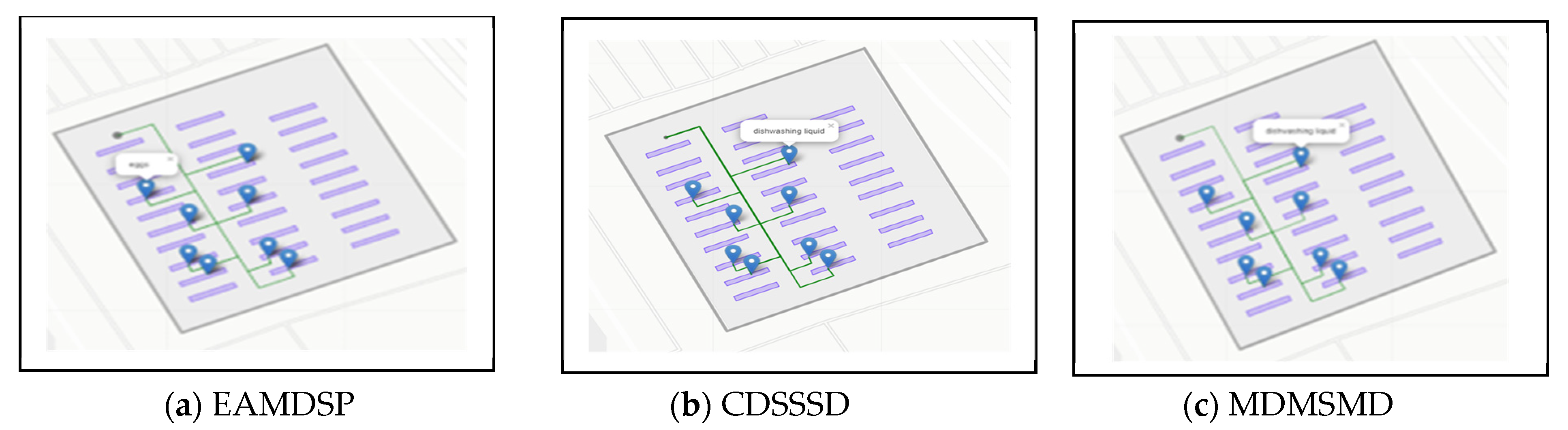
Dishwashing liquid	Cleaners
Eggs	Dairy
Mixes	Dry/Baking goods
Vegetables	Frozen foods
Pork	Meat

Figure 17a–c are supermarket simulation result of respectively EAMDSP, CDSSSD and MDMSMD which show the shortest path among eight items. Table 18 shows the output summary data for the eight-item search. When using EAMDSP for the shortest path between the above eight items, 58 nodes were visited and the total weight was 67. However, when using CDSSSD and MDMSMD for the same items, visited nodes were 104 and 72 and the total cost was 150 and 95, respectively. Therefore, EAMDSP is efficient for visited nodes and total weight. Finally, total visited nodes, or total cost can be expressed as EAMDSP < MDMSMD < CDSSSD.

Figure 17. Simulation on supermarket scenario using EAMDSP, CDSSSD, and MDMSMD for an eight-item search (output scenario).

Table 18. The output summary data of EAMDSP, CDSSSD, and MDMSMD for an eight-item search.

SL No.	Algorithm Name	Total Visited Nodes	Total Cost
1	EAMDSP	58	67
2	CDSSSD	104	150
3	MDMSMD	72	95

Table 19 represents the input values of the selected eleven items. These input items were used for the same simulation layout of three algorithms CDSSSD, MDMSMD, and EAMDSP.

Table 19. (Input) Selecting eleven items and categories.

Item	Category
Juice	Beverages
Dinner rolls	Bread/Bakery
Spaghetti sauce	Canned/Jarred goods
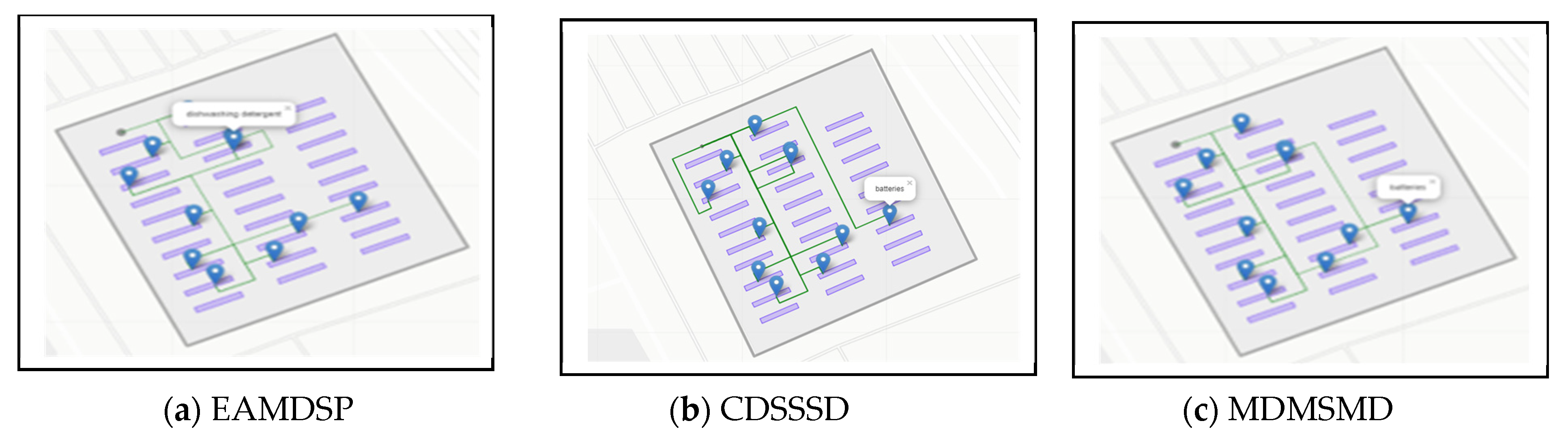
Dishwashing detergent	Cleaners
Cheeses	Dairy
Flour	Dry/Baking goods
Individual meals	Frozen foods
Lunch meat	Meat
Batteries	Others
Paper towels	Paper goods
Shampoo	Personal cares

Figure 18a–c are supermarket simulation result of respectively EAMDSP, CDSSSD and MDMSMD which show the shortest path among eleven items. Table 20 shows the output summary data for an eleven-item search. When using EAMDSP for the shortest path between the above eleven items, 78 nodes were visited and the total weight was 88. However, when using CDSSSD and MDMSMD for the same items the visited nodes were 124 and 101 and the total cost was 165 and 132 respectively. Therefore, EAMDSP is efficient for visited nodes and total weight. Finally, total visited nodes, or total cost can be expressed as EAMDSP < MDMSMD < CDSSSD.

Figure 18. Simulation on supermarket scenario using EAMDSP, CDSSSD, and MDMSMD for an eleven-item search (output scenario).

Table 20. Summary data of EAMDSP, CDSSSD, and MDMSMD for eleven items search.

SL No.	Algorithm Name	Total Nodes	Total Cost
1	EAMDSP	78	88
2	CDSSSD	124	165
3	MDMSMD	101	132

Figure 19 shows the cost-wise comparison among EAMDSP, CDSSSD and MDMSMD as per Table 21.

Figure 19. Cost-wise comparison between EAMDSP, CDSSSD, and MDMSMD.

Table 21. Total cost-wise comparison between EAMDSP, CDSSSD, and MDMSMD.

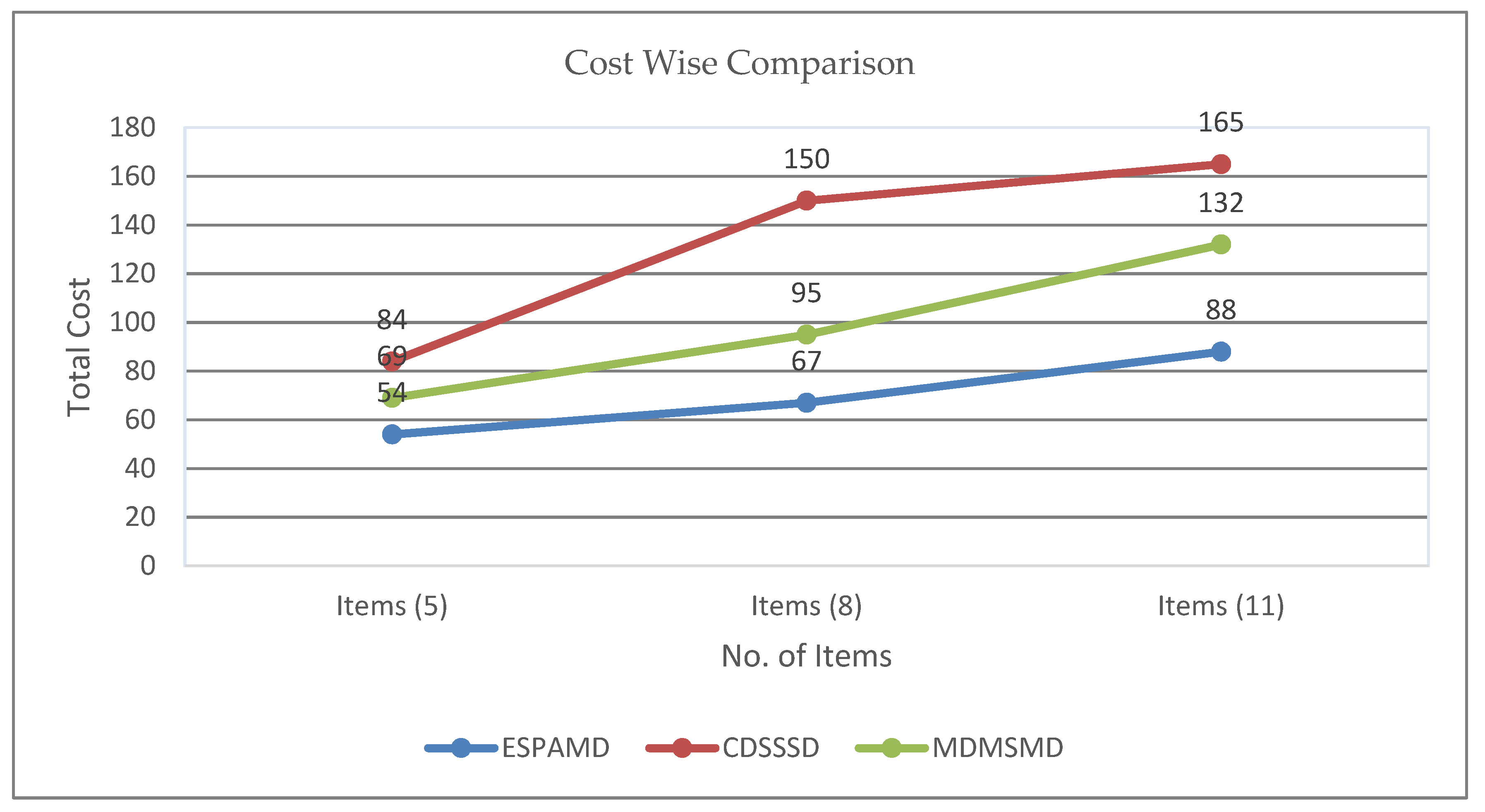
SL No.	Algorithm Name	Items (5)	Items (8)	Items (11)
1	EAMDSP	54	67	88
2	CDSSSD	84	150	165
3	MDMSMD	69	95	132

Figure 20 shows the visited-wise comparison among EAMDSP, CDSSSD and MDMSMD as per Table 22.

Figure 20. Visited node-wise comparison between EAMDSP, CDSSSD, and MDMSMD.

Table 22. Total visited node-wise comparison between EAMDSP, CDSSSD, and MDMSMD.

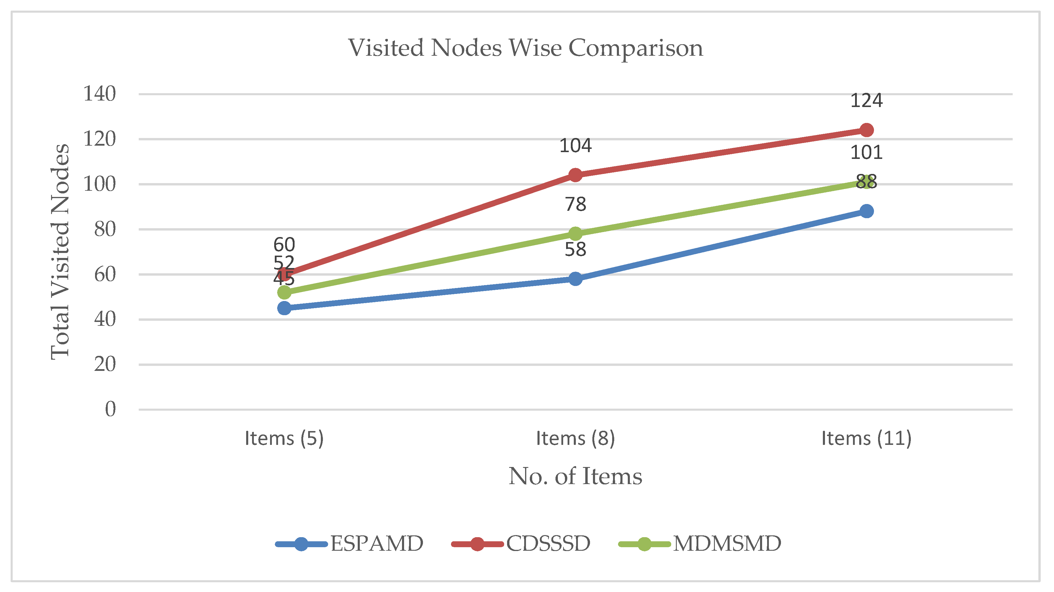
SL No.	Algorithm Name	Items (5)	Items (8)	Items (11)
1	EAMDSP	45	58	88
2	CDSSSD	60	104	124
3	MDMSMD	52	78	101

Finally, based on Figure 13, Figure 14, Figure 19 and Figure 20, and Table 13, Table 14, Table 21 and Table 22 it is reported that the proposed EAMDSP demonstrates the outstanding performance on cost and number of visited nodes compared to CDSSSD and MDMSMD.

5. Conclusions

The proposed EAMDSP algorithm was developed and implemented in indoor applications and found to be more efficient for a multi-destination search. It can be used on any type of road network with multi-destinations for shortest path searching. In this paper, we evaluated the EAMDSP by comparing it with CDSSSD and MDMSMD using two different simulations of several items of searching. For a search with a large number of products, EAMDSP demonstrated an outstanding performance compared to CDSSSD and MDMSMD, based on the total visited nodes and weights. The output of these simulations based on visited nodes and the minimum sum of weights is presented in tables and graphs. This research can be a useful guide for indoor shortest-path researchers. In future work, we might extend the application of EAMDSP from an indoor to an outdoor environment.

References

- Adamatzky, A. Shortest Path Solvers. From Software to Wetware; Springer: Berlin/Heidelberg, Germany, 2018; Volume 32. [Google Scholar]
- Papadopoulos, S.; Kompatsiaris, Y.; Vakali, A.; Spyridonos, P. Community detection in social media, performance and application considerations. J. Data Min. Knowl. Discov. 2012, 24, 515–554. [Google Scholar] [CrossRef]
- Kwon, Y.S.; Sohn, M.Y. Classification of Efficient Total Domination Sets of Circulant Graphs of Degree 5. Symmetry 2020, 12, 1944. [Google Scholar] [CrossRef]
- Yang, L.; Li, D.; Tan, R. Shortest Path Solution of Trapezoidal Fuzzy Neutrosophic Graph Based on Circle-Breaking Algorithm. Symmetry 2020, 12, 1360. [Google Scholar] [CrossRef]
- Kalaitzakis, A. Comparative Study of Community Detection Algorithms in Social Networks. Ph.D. Thesis, Technological Educational Institute of Crete, Heraklion, Greece, 1939. [Google Scholar]
- Bharath-Kumar, K.; Jaffe, J.M. Routing to Multiple Destinations in Computer Networks. IEEE Trans. Commun. 1983, 31, 343–351. [Google Scholar] [CrossRef]
- Ben Ticha, H.; Absi, N. A Solution Method for the Multi-Destination Bi-Objectives Shortest Path Problem; Elsevier: Amsterdam, The Netherlands, 2017. [Google Scholar] [CrossRef]
- Dong, Y.F.; Xia, H.M.; Zhou, Y.C. Disordered and Multiple Destinations Path Planning Methods for Mobile Robot in Dynamic Environment. J. Electr. Comput. Eng. 2016, 2016, 3620895. [Google Scholar] [CrossRef]
- Sepehrifar, M.K.; Zamanifar, K.; Sepehrifar, M.B. An Algorithm to Select the Optimal Composition of the Services. J. Theor. Appl. Inf. Technol. 2009, 8, 154–161. [Google Scholar]
- Wang, W.; Uehara, M.; Ozaki, H. Evaluation of navigation based on system optimal traffic assignment for connected cars. Int. J. Grid Util. Comput. 2020, 11, 525–532. [Google Scholar] [CrossRef]
- Burgaña, J.L. Design and evaluation of a link-state routing protocol for Internet-Wide Geocasting. Master’s Thesis, University of Twente, Enschede, The Netherlands, 2017. [Google Scholar]
- Sepehrifar, M.K.; Fanian, A.; Sepehrifar, B. Shortest Path Computation in a Network with Multiple Destinations. Arab. J. Sci. Eng. 2020, 45, 3223–3231. [Google Scholar] [CrossRef]
- Jubair, F.; Hawa, M. Exploiting Obstacle Geometry to Reduce Search Time in Grid-Based Pathfinding. Symmetry 2020, 12, 1186. [Google Scholar] [CrossRef]
- Rahman, M.S.; Ahmed, S. A survey on pairwise compatibility graphs. AKCE Int. J. Graphs Comb. 2020, 17, 788–795. [Google Scholar] [CrossRef]
- Easttom, W.; Adda, M. An enhanced view of incidence functions for applying graph theory to modeling network intrusions. WSEAS Trans. Inf. Sci. Appl. 2020, 15, 102–109. [Google Scholar]
- Cormen, T.H.; Leiserson, C.E.; Rivest, R.L.; Stein, C. Introduction to Algorithms; MIT Press: Cambridge, MA, USA, 2009. [Google Scholar]
- Arman, N.; Khamayseh, F. A Path-Compression Approach for Improving Shortest-Path Algorithms. Int. J. Electr. Comput. Eng. 2015, 5, 772–781. [Google Scholar] [CrossRef]
- Hakeem, A.; Gehani, N.; Ding, X.; Curtmola, R.; Borcea, C. Multi-destination vehicular route planning with parking and traffic constraints. In Proceedings of the 16th EAI International Conference on Mobile and Ubiquitous Systems: Computing, Networking and Services, Houston, TX, USA, 12–14 November 2019; pp. 298–307. [Google Scholar]
- Hu, W.-C.; Wu, H.-T.; Cho, H.-H.; Tseng, F.-H. Optimal Route Planning System for Logistics Vehicles Based on Artificial Intelligence. J. Internet Technol. 2020, 21, 757–764. [Google Scholar]
- Li, X.; Yin, H. Optimal Mobile Relays Positions and Resource Allocation for Multi-Relay Multi-Destination Wireless Networks. IEEE Access 2020, 8, 47993–48004. [Google Scholar] [CrossRef]
- Anđelić, M.; Živković, D. Efficient Algorithm for Generating Maximal L-Reflexive Trees. Symmetry 2020, 12, 809. [Google Scholar] [CrossRef]
- Zhang, H.; Zhang, Z. AOA-Based Three-Dimensional Positioning and Tracking Using the Factor Graph Technique. Symmetry 2020, 12, 1400. [Google Scholar] [CrossRef]
- Panić, B.; Kontrec, N.; Vujošević, M.; Panić, S. A Novel Approach for Determination of Reliability of Covering a Node from K Nodes. Symmetry 2020, 12, 1461. [Google Scholar] [CrossRef]
- Slamin, S.; Adiwijaya, N.O.; Hasan, M.A.; Dafik, D.; Wijaya, K. Local Super Antimagic Total Labeling for Vertex Coloring of Graphs. Symmetry 2020, 12, 1843. [Google Scholar] [CrossRef]
- Martínez, A.C.; García, S.C.; García, A.C.; Del Rio, A.M.G. On the Outer-Independent Roman Domination in Graphs. Symmetry 2020, 12, 1846. [Google Scholar] [CrossRef]
- Martínez, A.C.; Estrada-Moreno, A.; Rodríguez-Velázquez, J.A. Secure w-Domination in Graphs. Symmetry 2020, 12, 1948. [Google Scholar] [CrossRef]
- Lv, Y.; Liu, M.; Xiang, Y. Fast Searching Density Peak Clustering Algorithm Based on Shared Nearest Neighbor and Adaptive Clustering Center. Symmetry 2020, 12, 2014. [Google Scholar] [CrossRef]
- Balakrishnan, A.; Banciu, M.; Glowacka, K.; Mirchandani, P. Hierarchical approach for survivable network design. Eur. J. Oper. Res. 2013, 225, 223–235. [Google Scholar] [CrossRef]
- Fredman, M.L.; Tarjan, R.E. Fibonacci heaps and their uses in improved network optimization algorithms. J. ACM 1987, 34, 596–615. [Google Scholar] [CrossRef]
- Qu, T.; Cai, Z. A Fast Isomap Algorithm Based on Fibonacci Heap. In International Conference in Swarm Intelligence; Springer: Cham, Switzerland, 2015; pp. 225–231. [Google Scholar]
- Lu, X.; Camitz, M. Finding the shortest paths by node combination. Appl. Math. Comput. 2011, 217, 6401–6408. [Google Scholar] [CrossRef]
- Orlin, J.B.; Madduri, K.; Subramani, K.; Williamson, M. A faster algorithm for the single source shortest path problem with few distinct positive lengths. J. Discret. Algorithms 2010, 8, 189–198. [Google Scholar] [CrossRef]
- Thorup, M. Undirected single-source shortest paths with positive integer weights in linear time. J. ACM 1999, 46, 362–394. [Google Scholar] [CrossRef]
- Thorup, M. On RAM Priority Queues. SIAM J. Comput. 2000, 30, 86–109. [Google Scholar] [CrossRef]
- MacCormick, J. What Can Be Computed? A Practical Guide to the Theory of Computation; Princeton University Press: Princeton, NJ, USA, 2018. [Google Scholar]
- Xu, M.; Liu, Y.; Huang, Q.; Zhang, Y.; Luan, G. An improved Dijkstra’s shortest path algorithm for sparse network. Appl. Math. Comput. 2007, 185, 247–254. [Google Scholar] [CrossRef]
- Holzer, M.; Schulz, F.; Wagner, D.; Willhalm, T. Combining speed-up techniques for shortest-path computations. ACM J. Exp. Algorithmics 2005, 10, 2–5. [Google Scholar] [CrossRef]
- Chen, Y.-Z.; Shen, S.-F.; Chen, T.; Yang, R. Path Optimization Study for Vehicles Evacuation based on Dijkstra Algorithm. Procedia Eng. 2014, 71, 159–165. [Google Scholar] [CrossRef]
- Madkour, A.; Aref, W.G.; Rehman, F.U.; Rahman, M.A.; Basalamah, S. A survey of shortest-path algorithms. arXiv 2017, arXiv:1705.02044. [Google Scholar]
- Okengwu, U.A.; Nwachukwu, E.O.; Osegi, E.N. Modified Dijkstra algorithm with invention hierarchies applied to a conic graph. arXiv 2015, arXiv:1503.02517. [Google Scholar]
- Hong, Y.; Li, D.; Wu, Q.; Xu, H. Priority-Oriented Route Network Planning for Evacuation in Constrained Space Scenarios. J. Optim. Theory Appl. 2019, 181, 279–297. [Google Scholar] [CrossRef]
- Jin, W.; Chen, S.; Jiang, H. Finding the K shortest paths in a time-schedule network with constraints on arcs. Comput. Oper. Res. 2013, 40, 2975–2982. [Google Scholar] [CrossRef]
- Ananta, M.T.; Jiang, J.-R.; Muslim, M.A. Multicasting with the extended Dijkstra’s shortest path algorithm for software defined networking. Int. J. Appl. Eng. Res. 2014, 9, 21017–21030. [Google Scholar]