Abstract
A moving meshing algorithm with mesh adaptive size function was proposed in this paper with regard to the modeling speed and solution accuracy of electromagnetic equipment in the optimization design process. In the proposed method, a mesh size function that considers curvature, feature size, and distance gradient restrictions is constructed, which can obtain high quality meshes and avoid excessive iteration; when the finite element mesh domain is deformed, only the mesh nodes close to the moving boundary are allowed to move, and the theory of force-balance is used combined with the second-order boundary projection algorithm to perform iterative optimization of the mesh node positions. The proposed method has the advantages of keeping the original mesh structure and minimum mesh deformation as well as speed up the convergence, save time in the finite element meshing, and ensure the quality of the generated mesh. Then, the proposed method was applied to a 37 kw motor for electromagnetic analysis, and the results obtained proved the accuracy of the algorithm; finally, the effectiveness of the mesh movement algorithm in three-dimensional space was tested by moving the sphere inside the cylinder.
1. Introduction
In recent decades, the finite element method (FEM) has become the main solution method for solving partial differential equations PDE. The core step of FEM is to divide the geometric domain into mesh elements that conform to the FEM solution rules. There is no doubt that the quality of mesh elements is crucial to the accuracy of the solution [1]. When using FEM, the prerequisite for obtaining discrete solutions of continuous problems described by partial differential equations (PDE) and boundary/initial conditions is that a computational mesh must be generated to define unknowns [2,3].
Generally, mesh generators can easily generate meshes without writing any programming code, but the ability to comprehend and optimize meshing algorithms is a worthwhile choice, just like geometric modeling and data mining and analysis in computer graphics. After decades of development, the field of finite element mesh generation has developed rapidly, and many important technologies and algorithms have emerged. Modern mesh generation technologies are mainly divided into three categories: advancing-front methods [4,5], mesh-overlay techniques [6,7], and Delaunay-based approaches [8,9]. Essential research has also focused on the development of mesh improvement technology, aiming at improving the quality of the existing mesh [10,11,12].
At present, there are open source unstructured meshing algorithms such as Distmesh, Gmsh, Mesh2d, Triangle, etc. These algorithms have promoted the development of meshing technology [13,14,15]. However, these algorithms have room for further improvement such as mesh size adaptation, mesh deformation processing, and the multi-subdomain definition, which need to be improved to adapt to actual finite element analysis scenarios.
Unstructured mesh generation technology uses different element sizes to resolve the features of the geometry, but uses coarse meshes to cut down the total mesh size when possible [14]. For many mesh generation algorithms, it is favorable if the appropriate mesh size function h(x) is known before generating the mesh [16]. Many techniques for automatically generating mesh size functions have been proposed. The authors in [13,14] studied whether different adaptive mesh refinement strategies with suspended nodes were allowed, and the focus was on improving the data structure. The study by [17,18,19] proposed a novel heuristic posterior error estimator, combined with mesh refinement and mesh coarsening. This method requires special attention to the numerical error solution. The authors [20] proposed a method suitable for an adaptive mesh refinement algorithm for elliptic partial differential equations. The algorithm combines posterior error estimation and the bubble-type local mesh generation (BLMG) method to ensure that the errors are evenly distributed on the triangle. The study in [21] proposed an adaptive mesh generation method that used node-based local meshes to discrete incompressible flows, and [22] proposed the use of the element-free Galerkin method for adaptive analysis. However, like all of the other physics-based methods, the cost of generating high-quality meshes is high.
For the actual electromagnetic analysis field, in order to improve the performance of electromagnetic equipment, it is necessary to continuously optimize the analysis during the design process. The basis of electromagnetic equipment optimization analysis is the outstanding quality of the mesh elements, which require mesh optimization. In fact, mesh optimization is also necessary in other problems, not only in electromagnetic analysis. One example is the modeling of the welding thermal effects [23]. This is also essential for further research on predictive maintenance tasks related to electromagnetic equipment [24,25]. During the optimization process, the finite element field will change. Generally, the new mesh can be obtained by completely retriangulating or by solving the elastic function [26], Laplace function [27], or biharmonic function to update the previous mesh [28]. However, these full or partial remeshing methods are consuming. In addition, for partial remeshing strategies, using differential equation (PDE) methods to disperse the design boundary changes to adjacent nodes may generate folded or inverted mesh elements, resulting in invalid meshing [29]. In order to solve these problems more effectively, some authors have proposed other methods [30,31] such as mesh deformation based on radial basis function interpolation and optimized moving meshing strategy. The numerical formulas of both methods are complicated as they must match their solutions between the meshes to ensure that the overall solution is continuous. In order to overcome the shortcomings of the above methods in making meshes for new geometric parameters, a parameterized mesh technology was proposed, improved, and optimized to achieve rapid two-dimensional mesh deformation [32,33,34]. This method finds it difficult to generate meshes for the boundaries of complex geometric domains, and it is easy to generate mesh elements of lower quality.
This paper proposes a novel meshing algorithm for finite element analysis. The algorithm uses a signed distance function to define the geometric area, and calculates the boundary curvature and approximate medial axis through the signed distance function to construct a mesh size function, and then applies a mesh size restriction function based on the distance function and gradient to obtain a smoother mesh size function processing effect and accurate projection of internal boundary points through the second-order projection method, which makes it possible to solve discontinuous material coefficients in finite element calculations. When the geometric area changes, by assigning the edge stiffness of each mesh cell, selective iterative optimization can greatly reduce the calculation time and maintain a high-quality mesh.
2. Mesh Generation Theory
This paper intends to optimize the mesh generation algorithm based on Distmesh, and the representation of the geometric domain is specified and described by using the signed distance function [15]. In addition, the gradient of the distance function points to the direction of the boundary, which will effectively project the nodes near the boundary that meet the requirements of the boundary point onto the boundary. The implicit geometric domain Ω can be expressed as:
For example, consider the space curve x2 + y2 = 1 on the two-dimensional plane, as shown in Figure 1. The zero-level function of ϕ(x, y) = x2 + y2 − 1 is ϕ(x, y) = 0, that is, ∂Ω = {(x, y)|ϕ(x, y) = 0}, which is exactly the same. In this case, the inner area is Ω− = {(x, y)|x2 + y2 < 1}, the boundary of the area is Ωe = {(x, y)|x2 + y2 < 1}, and the outer area is Ω+ = {(x, y)|x2 + y2 > 1}. These areas are shown below:
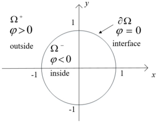
Figure 1.
Implicit representation of the curve x2 + y2 = 1.
For the generation process of mesh elements, see [23]. The iterative mesh optimization technology is based on the physical analogy between the mesh element edges and the truss structure, and the mesh nodes are the nodes of the truss. Assuming that the bar element in the truss has an appropriate force in each iteration, corresponding to the edge of the mesh element, it is necessary to solve the force balance problem, and then move the node through the force. The force-balance function corresponds to a nonlinear equation.
The force balance function can be solved based on the artificial time dependence. For some p(0) = p0, Equation (2) can be a fixed solution of the ordinary differential equation (ODE) (non-physical) system.
After obtaining a stable solution that satisfies Equation (2), when the discrete time tk = kΔt is set, the approximate solution pk ≈ p(tk) will be updated as follows:
Reference [35] sets each edge to have a lij = [pi, pj] variable spring constant f(pi, pj), which depends on the current length of the mesh element edge ||lij|| and the desired ideal length eij. By adopting the concept of normalized length and defining sij = ||lij||/eij, the force balance function f can be expressed as:
3. The Proposed Meshing Method for Finite Element Analysis
In this paper, based on the requirements and characteristics of finite element analysis, an adaptive mesh size function considering curvature, feature size, and distance gradient restriction was constructed; the second order projection algorithm was used to define the internal common boundary between different materials to meet the actual application of finite element; a novel moving meshing algorithm suitable for large deformation was proposed, and a mesh smoothing function based on bar force-balance was used to smooth the mesh, which reduces the mesh iteration time and ensures the quality of mesh generation.
In order to measure the quality of the mesh, this paper introduces Equation (6). According to the empirical criterion, 0.5 < q < 1, the mesh quality is considered as favorable; when q = 1, the triangle is an equilateral triangle, which is the most idealized mesh element [36]:
where a, b, and c are the lengths of the three sides of the triangle element under consideration; Δ is its area.
3.1. Curvature and Approximate Medial Axis Based Mesh Size Function
The unstructured mesh generation algorithm uses different mesh cell sizes to solve the subtle features in different regions. The mesh size function h(x) is generally described by some factors. In the process of mesh size adaptation in the curved boundary, the h(x) function should be small to adapt to curvature changes. For areas with small local feature sizes, it is recommended using smaller elements to stroke well-shaped elements. Finally, the mesh size function is smoothed to prevent unnecessary mesh iteration. This article will limit it based on the ∇h(x)/distance function.
Provide a method to automatically solve the mesh size function in the domain, which is an essential part of mesh generation.
3.1.1. Curvature Based Mesh Size Function
In order to accurately solve the value near the boundary of the curve, it was planned to impose a curvature limit on the boundary: h(x) ≤ hc(x). For the unstructured background mesh, the value of h(x) was specified on the boundary node, and the value of the remaining nodes was set to infinity. Later, these values can be uniformly propagated to other locations in the mesh domain through distance gradient constraints. It is recommended to use a closed form of curvature expression, which will improve the calculation accuracy and speed. The boundary curvature κ(x) is solved by a defined distance function. Compared with the method of using edge advance-Delanuany, this method is easier to use and avoids the problem of numerical inaccuracy that may be caused by the ordering of edges.
The mesh size function based on curvature can be obtained:
where κ(x) is the curvature at x; h0(x) is the initial mesh size function; and ∆x is the resolution of the background meshes. By adding ∆x to limit the size of the edge of the narrow band that may appear near the area in order to deal with the possible high curvature problem, this method will not affect the interior of the area as the coupling process with other mesh size functions can avoid the waste of computing resources.
Use Equation (6) to calculate the quality of mesh elements. Figure 2a is obtained by using the mesh size function without curvature restriction. As can be seen from Figure 2c, the minimum quality of the generated mesh was 0.82 and the average quality was 0.94. Figure 2b was obtained by using the mesh size function with curvature restriction. As can be seen from Figure 2d, the minimum quality of the generated mesh was 0.63 and the average quality was 0.91. While increasing the mesh density at the boundary of the curve, the average quality of the mesh is ensured to meet the requirements of the accurate finite element solution.
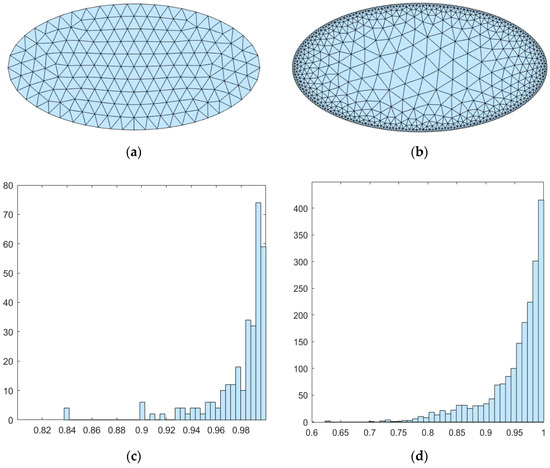
Figure 2.
Validation of the mesh size function based on curvature. (a) Mesh generation without hc(x); (b) mesh generation with hc(x); (c) mesh quality map without hc(x); and (d) mesh quality map with hc(x).
3.1.2. Medial Axis Set Based Mesh Size Function
For local feature size adaptation, we planned to apply a condition h(x) ≤ hm(x) anywhere in the domain. The local feature size is measured based on the distance between neighboring boundaries. The local feature size of the boundary node p is approximately similar to the shortest distance between the node p and the intermediate axis. The middle axis is a special set of internal points, where the internal points in the set are at the same distance from at least two points on the boundary of the geometric domain. For the sake of saving time, this paper used the approximate medial axis set, that is, by finding the local extremum in ∇ϕ(x), it is equivalent to defining the position of the intermediate point ‘m’ as the position satisfying and and ϕ(x) <0. It must be noted that ϕ(x) should be a piecewise smooth distance function, then the signed distance function ϕ(x) is differentiable, and each point that is differentiable should satisfy . For any node p that is satisfied, the distance to the intermediate axis will be defined as ϕm(x) = ϕ(x, m). The local feature size function hm based on the approximate intermediate shaft is calculated as follows:
where h0 is the initial mesh size specified by the user, and kt is the scale factor of the middle axis. Generally, users use h0 as the benchmark, preset the number of elements required by the local feature size, and then determine the kt value, and ϕm is the absolute distance to the nearest medial point. The approximate medial axis is used to calculate the mesh size function, which adapts to the characteristics of the geometric domain and avoids computational complexity. There is no doubt that the mesh size function generated based on the intermediate axis is also applicable to geometric domains with similar branch pipe shapes. It is only necessary to find the set of points in the area that conform to the definition of the medial axis to generate a structured mesh with topological characteristics, which will facilitate analysis and comparison between different parts of the finite element domain.
Use Equation (6) to calculate the quality of mesh elements. From Figure 3c, it can be clearly seen that the mesh quality without the local feature size function hm(x) was the lowest 0.65 and the average mesh quality was 0.94. Using the local feature size function hm(x), the mesh quality was the lowest at 0.71, and the average mesh quality was 0.94. The local feature size function based on the approximate medial axis can ensure the average mesh quality of the mesh and meet the requirements of the accurate finite element solution.
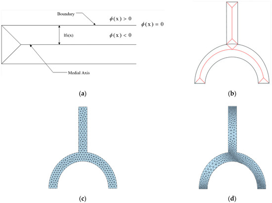
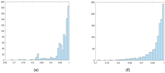
Figure 3.
Verification of the mesh size function based on hm(x). (a) Signed distance function ϕ(x); (b) the approximate medial axis of Sandia Fork; (c) mesh quality map without hm(x); (d) mesh quality map with hm(x); (e) mesh quality map without hm(x); and (f) mesh quality map with hm(x).
3.2. Distance Gradient Limiting Function
For the meshing process, it is necessary to specify the minimum and maximum mesh sizes hmin and hmax, and h0(x) should be between them
The global mesh size function is calculated according to curvature, local feature size function based on approximate medial axis, and user-defined mesh size function
The dimension function hext(x) is provided as user input.
For the actual effect of the mesh size function, it is necessary to ensure that the ratio of the generated adjacent mesh element sizes is less than the given value g. Regarding how to meet this requirement, consider limiting the gradient of the mesh size function. This article requires h(x) ≤ hg(x), which can be satisfied by finding the steady-state solution of the so-called gradient limit equation [15],
initial condition
The results are as follows:
Among them,
Obviously, the smoothly changing mesh size function is consistent with the improved element quality, which can avoid excessive mesh iteration to a certain extent.
An idealized model can be constructed to represent the effect of both the element shape quality and the gradient limit of the size function. A normal triangle with standard edge length l and (1 + g)l is considered. g is solved according to the minimum angle θmin in the triangle. Using the angle to solve g can maximize the calculation error caused by the mesh superposition or distortion. Compared with solving the steady-state solution of the gradient limit equation, this method is a simple and efficient strategy.
where i,j ∈ (1,2,3). Obviously, g→0 corresponds to θmin→60.0° and g = 0.3 corresponds to θmin = 45.0°. The specific functions are as follows:
xi,xj ∈ Ω, where xj can only be smoothed from adjacent points xi ∈ Ω, and its premise is h(xi) < h(xj), which can be guaranteed by the distance function.
It is planned to use the distance function as the benchmark to adapt to its geometric complexity. If the mesh resolution transition is not uniform, the mesh quality will be affected. Therefore, the mesh size function is equal to the linear growth of the user-defined mesh initial size function h0(x) and the signed distance function ϕ(x), which may be appropriate:
where α0 is the percentage change of the mesh size with the boundary.
The limit function of distance gradient is as follows:
In order to highlight the necessity of gradient restriction, the distance gradient restriction function is only combined with the mesh size function input by the user to verify its effect and make a comparison (h0 = 0.1). Use Equation (6) to calculate the quality of mesh elements.
From Figure 4, it can be clearly seen that the mesh size function could obtain few poor mesh cells without using the distance gradient function, and the worst mesh quality can be obtained from Table 1, which was 0.0219. However, applying the distance gradient function to the mesh size function could make the mesh size smoother, reduce the mesh iteration by 40%, increase the speed by 33%, and generate the lowest mesh quality of 0.546.
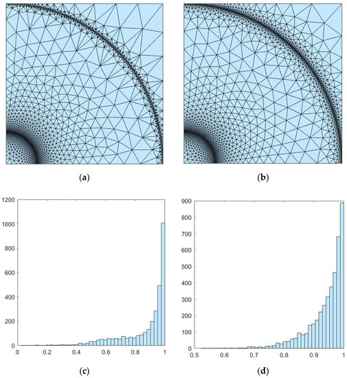
Figure 4.
Validation of mesh size function based on distance gradient constraint. (a) mesh generation without hgd(x); (b) mesh generation with hgd(x); (c) mesh quality map without hgd(x); (d) mesh quality map with hgd(x).

Table 1.
Validation of mesh size function based on distance gradient restriction.
3.3. Moving Meshing Algorithm
Considering that the design process involves thousands of shape changes, complete remeshing is time-consuming. In order to speed up the finite element analysis, a novel moving meshing algorithm is proposed.
3.3.1. Second Order Projection Algorithm
In the finite element calculation, the situation of internal multiple subdomains is very likely to be encountered, which requires exploring the definition of internal boundaries in finite element meshing.
As for how to define the internal boundary, one method is to mesh the relevant parts of the domain before all the domains are meshed, and fix the positions of the generated nodes and boundary elements; on this basis, the other domains are meshed. This method is essentially a bottom-up method, which relies too much on more human intervention. If the boundary is not fixed or complex, it cannot be defined accurately.
In this paper, the implicit signed distance function ϕ(x) was used to express the inner boundary ϕ. For the outer boundary, this paper used Equation (20) to project until ‖ϕ(p)‖ became small enough:
As for how to define the internal boundary, this article discusses approximating the estimate by assuming an implicit function ϕ. The higher-order approximate formula projection can be obtained by spreading more in the truncated Taylor expansion of ϕ. In this paper, only two-dimensional planes were considered. For a node (x, y) and a tiny displacement (∆x, ∆y),
Among
Figure 5 is a comparison of the difference between the first-order projection and the second-order projection. Project a point onto ϕ = y − sin(3πx). Repeat the projection until the projection point is close to boundary ϕ. It can be seen that the first-order projection strategy is to let the node move in the gradient direction first, then move toward the boundary, which will cause the projection to be inaccurate because it will deviate from the true projection position; this can be clearly seen in Figure 5. The second-order projection method moves the node directly toward the boundary, which is a more accurate projection.
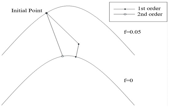
Figure 5.
First-order projection and second-order projection schemes.
3.3.2. Dynamic Technology
First, the problem of boundary definition in the process of finite element subdivision domain change is solved. In Section 3.3.1, we introduced the geometric definition method involving external boundary and internal boundary. Then, according to the velocity field v(x), the geometric boundary is evolved in time. After the evolution of ϕ, the signed distance function is usually not retained and needs to be reinitialized in the same way as the initial signed distance function is calculated. In general, ϕ(x) is suggested to be expressed in closed form, which will avoid the problem of non-termination of iteration due to complex boundary conditions.
Next, enter the mesh operation phase. For the mesh obtained in the previous step, set it as the initial mesh in this step. We can delete the elements that are not in the domain at all. The distance function can be used to detect nodes, the sufficient condition is that ϕ(x) > 0. After optimization, if ϕ(x) > 0 at the centroid of the element, the external element is removed. In order to ensure that the boundary points will not be deleted by mistake, according to the mesh density function h(x), a random number of 0–1 is generated on each point to determine whether it is less than r0/max(r0), where r0 = [h(px)]−2. If it is greater than, the point is deleted. In this way, the quality of boundary elements can be guaranteed to a large extent.
Using the linear spring model to push out nodes [23]:
where sij = ||lij||/eij and ||lij|| is the current mesh element length, and the desired length is eij.
After the initial mesh is obtained, the operation of the moving mesh algorithm is started. The idea of the moving meshing algorithm is to apply a certain stiffness to the edge of each mesh element according to the signed distance function value of each node. The stiffness decreases as the distance from the active interface increases, which will ensure that the mesh elements far away from the active interface remain basically unchanged. Then, when solving the force balance, they can be ignored, thus significantly improving the performance. For the elements adjacent to the motion interface, according to ϕ(x) in the update iteration process, determine whether to project onto the boundary, and the smoothing iteration is performed:
Use Equation (6) to calculate the quality of mesh elements. q is the mesh element quality, qavg is the average of the quality of the entire meshes, ϕi is the distance function expression of moving boundary, and ϕ is the distance function expression of the fixed boundary.
In this paper, Equation (3) and p(0) = p0 were used for the novel moving meshing algorithm. Approximately solve Equation (3) with the pre-Euler method. pik is set to the position of node i in the k time step, provided that the discrete time tk = kΔt is set. In order to get the steady state, the node position is updated iteratively by Equation (26).
where rij is the expected mesh edge length and eij is the actual mesh edge length. Ni is the neighborhood of node i.
The node position in the moving mesh is updated by Equation (26). Iterative equations are particularly useful for moving mesh, and only a few iterations are needed in each step to get favorable meshes. The idea of the moving meshing algorithm is also applicable to the three-dimensional field. Compared with solving differential equations or elastic equations and radial basis interpolation methods, the method proposed in this paper is simple to implement. It is based on the distance function to determine the position of the node to be moved and perform the movement operation, which will help improve the efficiency of the deformation domain processing. Additionally, its realization effect is slightly better than parametric mesh technology.
4. Validation Analysis
Computer configuration: Intel(R)Core(TM)i5-7500 CPU @ 3.40GHZ.
4.1. Verification of 2D Moving Mesh
To try to apply the proposed algorithm to the field of electromagnetic fields, a 37 kW, four-pole cage induction motor machine was simulated. The specific parameters of the motor are shown in Table 2 [37].
Table 2.
Motor data.
First, the mesh was divided into the following: Figure 6a is the mesh of the motor when the shaft is 45 mm and Figure 6b is the mesh of the motor when the shaft is 35 mm. For a motor with a shaft radius of 35 mm, two methods were used to mesh: one was to use the moving meshing algorithm based on the mesh data obtained by the original shaft radius of 45 mm; the other was to directly remodel the motor with a shaft radius of 35 mm, and use the algorithm in this paper to perform complete meshing based on this (h0 = 0.6). Use Equation (6) to calculate the quality of the mesh elements.
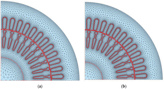
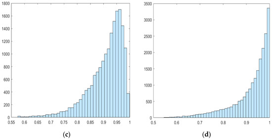
Figure 6.
Verification of the moving mesh algorithm. (a) Mesh generation with a 45 mm shaft radius; (b) mesh generation with a 35 mm shaft radius; (c) mesh quality map with a 45 mm radius of the rotating shaft; (d) mesh quality map of the shaft radius of 35 mm (moving meshing algorithm).
For this example, it took 20.12 s to mesh a motor with a shaft radius of 45 mm. On this basis, it can be seen from Table 3 that it only takes 1.41 s to generate a meshing map of a motor with a shaft of 35 mm; however, it takes 20.29 s to regenerate the meshing diagram of the motor with a 35 mm shaft. It is clear that the proposed method takes relatively less time. As can be seen from Figure 6c,d, the quality of the mesh elements generated by the novel algorithm was above 0.5, and the mesh quality was high, with more than 70% of the mesh quality above 0.8. After the moving meshing algorithm was processed, the mesh quality was still above 0.5, which is beneficial to the finite element solution. Compared with the parameterized mesh technology, the moving mesh algorithm proposed in this paper increased the speed by 20%, and there were no elements with a mesh element quality less than 0.5.
Table 3.
Solution results of different algorithms (shaft radius of 35 mm).
The induction motor was selected after the shaft was deformed for simulation processing. A quarter of the 37 kW induction motor was analyzed by taking into account the non-linearity of iron, and including the voltage equations of the stator winding and the rotor cage. For simplicity, the stator winding was modeled as an infinite number of strands, that is, the eddy current was not included outside the rotor cage. The finite element analysis based on the mesh data generated by the moving mesh algorithm was performed using 20,953 triangular elements and 10,637 nodes. The electrical period was divided into 200 time steps, which requires approximately 43 s of calculation time. To re-model, according to 35 mm to carry out the mesh generated by meshing to carry out the finite element analysis, 935 triangle elements and 10,629 nodes were used, and the same electrical period divided into 200 time steps took about 44 s calculation time. The rotor rotation was simulated by resetting the air gap elements at each time step.
Take a quarter of the motor center as the origin of the coordinate system, and set the unit coordinate length to 1 m. The electromagnetic analysis diagram is shown in Figure 7. The flux density (unit: T) was verified by selecting four nodes, and the comparison results are shown in Table 4.
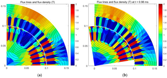
Figure 7.
Electromagnetic analysis (a) flux lined and flux density from time-harmonic analysis; (b) time-stepping simulation continued from the time-harmonic solution.
Table 4.
Solution results of various methods.
The results of the randomly selected points were compared and verified with the results of commercial finite element software, which proved the validity of the calculation results of the algorithm. Comparing the results of the FEA using the mesh generated by the moving mesh algorithm with the results of the FEA using the mesh generated without the moving meshing algorithm, it can be seen that the results of the two FEA methods were similar, and the accuracy was not greatly affected. It can be concluded that the mesh elements generated based on the moving meshing algorithm qualified for the finite element analysis, and greatly reduced the finite element meshing time and improved the efficiency of the finite element analysis. It is worth mentioning that the algorithm can also be extended to other engineering applications.
4.2. 3D Moving Mesh Verification
As a simple verification case of a three-dimensional moving meshing algorithm, this paper engaged a sphere passing through a cylinder. The initial radius was 0.5, the initial sphere center was (0, 0, 0), the radius was 0.7 after the change, and the sphere center coordinates remained unchanged (h0 = 0.1). We used Equation (6) to calculate the quality of the mesh elements.
According to the test, in a three-dimensional cylinder, there was a sphere with a sphere center (0, 0, 0) and a radius of 0.5. Its meshing diagram is shown in Figure 8a. It can be seen from Table 5 that it took 7.84 s and the number of mesh iterations was 76. As shown in Figure 8c, the mesh quality was greater than 0.5, when the radius became 0.7, the mesh was generated on the basis of the original radius of 0.5, and Figure 8b is obtained. It took 2.01 s, the number of mesh iterations was 37, and the mesh quality was greater than 0.55. Compared with the parameterized mesh technology, the speed of the algorithm in this paper was increased by 27%, and there were no mesh elements with a quality less than 0.5. The verification showed that the moving meshing algorithm proposed in this paper is also effective in the three-dimensional field, which can save the time of re-meshing, and its mesh quality can still be maintained.
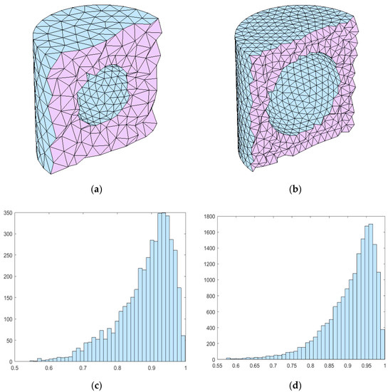
Figure 8.
Three dimensional verification of the moving meshing algorithm. (a) Original 3-D mesh (radius 0.5); (b) mesh generation by moving meshing algorithm (radius 0.7); (c) the original 3-D mesh quality map; (d) mesh quality map of radius 0.7 (moving meshing algorithm).
Table 5.
Solution results of different algorithms (3D moving mesh verification).
5. Conclusions
Aiming at the optimization design of electromagnetic equipment, a moving meshing algorithm with mesh adaptive size function was proposed. The algorithm constructs an adaptive mesh size function that considers curvature, feature size, and imposes distance gradient restrictions. On the basis of a second-order projection algorithm to define the internal common boundary between different materials, a novel moving meshing algorithm suitable for larger deformations was proposed, supplemented by a mesh smoothing function based on force-balance as mesh smoothing reduces the mesh iteration time while ensuring the quality of the generated mesh. A numerical example of a motor was given to verify the accuracy and efficiency of the algorithm; finally, a simple three-dimensional example was given to verify the effectiveness of this algorithm in three dimensions.
Author Contributions
Conceptualization and methodology, C.Z. and S.A.; Software, C.Z. and D.L.; Validation, C.Z., W.W., and D.L.; Writing—original draft preparation, C.Z. and S.A.; Writing—review and editing, W.W. and D.L.; Funding acquisition, S.A. All authors have read and agreed to the published version of the manuscript.
Funding
This research was funded by the National Natural Science Foundation of China (grant nos. 52077203) and the Natural Science Foundation of Zhejiang Province, China (grant no. LY19E070003).
Institutional Review Board Statement
Not applicable.
Informed Consent Statement
Not applicable.
Data Availability Statement
Not applicable.
Conflicts of Interest
The authors declare no conflict of interest.
References
- Nguyen, H.N.; Canh, T.N.; Thanh, T.T. Finite element modelling of a composite shell with shear connectors. Symmetry 2019, 11, 527. [Google Scholar] [CrossRef]
- Guo, W.; Nie, Y.; Zhang, W. Acceleration strategies based on bubble-type adaptive mesh refinement method. Math. Comput. Simul. 2020, 170, 143–163. [Google Scholar] [CrossRef]
- Zhao, Y.; Xiao, X.; Xu, W. Accelerating the Optimal Shape Design of Linear Machines by Transient Simulation Using Mesh Deformation and Mesh Connection Techniques. IEEE Trans. Ind. Electron. 2018, 65, 9825–9833. [Google Scholar] [CrossRef]
- Lo, S.H. A new mesh generation scheme for arbitrary planar domains. Int. J. Numer. Methods Eng. 1985, 21, 1403–1426. [Google Scholar] [CrossRef]
- Peraire, J.; Vahdati, M.; Morgan, K.; Zienkiewicz, O.C. Adaptive remeshing for compressible flow computations. J. Comput. Phys. 1987, 72, 449–466. [Google Scholar] [CrossRef]
- Shephard, M.S. Approaches to the automatic generation and control of finite element meshes. Appl. Mech. Rev. 1988, 1, 169–185. [Google Scholar] [CrossRef]
- Thacker, W.C. A brief review of techniques for generating irregular computational grids. Int. J. Numer. Methods Eng. 1980, 15, 1335–1341. [Google Scholar] [CrossRef]
- Bowyer, A. Computing Dirichlet tessellations. Comput. J. 1981, 24, 162–166. [Google Scholar] [CrossRef]
- Zhang, W.; Nie, Y.; Cai, L.; Qi, N. An adaptive discretization of incompressible flow using node-based local meshes. Comput. Model. Eng. Sci. 2014, 102, 55–82. [Google Scholar]
- Field, D.A. Laplacian smoothing and Delaunay triangulations. Commun. Appl. Numer. Methods 1988, 4, 709–712. [Google Scholar] [CrossRef]
- Frey, W.H.; Field, D.A. Mesh relaxation: A new technique for improving triangulations. Int. J. Numer. Methods Eng. 1991, 31, 1121–1133. [Google Scholar] [CrossRef]
- Engwirda, D. Locally-Optimal Delaunay-Refinement and Optimisation-Based Mesh Generation. Ph.D. Thesis, School of Mathematics and Statistics, The University of Sydney, Sydney, Australia, September 2014. [Google Scholar]
- Funken, S.A.; Schmidt, A. Adaptive Mesh Refinement in 2D—An Efficient Implementation in Matlab. Comput. Methods Appl. Math. 2019, 20, 459–479. [Google Scholar] [CrossRef]
- Funken, S.A.; Schmidt, A. A Coarsening Algorithm on Adaptive Red-Green-Blue Refined Meshes. arXiv Prepr. 2020, arXiv:2001.06343. [Google Scholar] [CrossRef]
- Persson, P.-O.; Strang, G. A Simple Mesh Generator in MATLAB. SIAM Rev. 2004, 46, 329–345. [Google Scholar] [CrossRef]
- Roberts, K.J.; Pringle, W.J.; Westerink, J.J. On the automatic and a priori design of unstructured mesh resolution for coastal ocean circulation models. Ocean Model. 2019, 144, 101–509. [Google Scholar] [CrossRef]
- Zhao, Y.; Zhang, X.; Ho, S.L.; Fu, W. An Adaptive Mesh Method in Transient Finite Element Analysis of Magnetic Field Using a Novel Error Estimator. IEEE Trans. Magn. 2012, 48, 4160–4163. [Google Scholar] [CrossRef]
- Zhao, Y.; Ho, S.L.; Fu, W. A Novel Adaptive Mesh Finite Element Method for Nonlinear Magnetic Field Analysis. IEEE Trans. Magn. 2013, 49, 1777–1780. [Google Scholar] [CrossRef]
- Zhao, J.; Li, S. Adaptive mesh refinement method for solving optimal control problems using interpolation error analysis and improved data compression. J. Frankl. Inst. 2020, 357, 1603–1627. [Google Scholar] [CrossRef]
- Zhang, W.; Nie, Y.; Gu, Y. Adaptive finite element analysis of elliptic problems based on bubble-type local mesh generation. J. Comput. Appl. Math. 2015, 280, 42–58. [Google Scholar] [CrossRef]
- Elliot, R.; Qiu, L.; Yu, Y.; Fedkiw, R. An adaptive discretization of incompressible flow using a multitude of moving Cartesian grids. J. Comput. Phys. 2013, 254, 107–154. [Google Scholar]
- Hagihara, S.; Motoda, S.; Tsunori, M.; Ikeda, T.; Miyazaki, N. Adaptive meshfree method based on adding and moving nodes. Int. J. Comput. Methods 2006, 3, 429–443. [Google Scholar] [CrossRef]
- Fratini, L.; Macaluso, G.; Pasta, S. Residual stresses and FCP prediction in FSW through a continuous FE model. J. Mater. Process. Technol. 2009, 209, 5465–5474. [Google Scholar] [CrossRef]
- Petrillo, A.; Picariello, A.; Santini, S.; Scarciello, B.; Sperli, G. Model-based vehicular prognostics framework using Big Data architecture. Comput. Ind. 2020, 115, 103–177. [Google Scholar] [CrossRef]
- Galli, A.; Gravina, M.; Moscato, V.; Sperli, G. Deep Learning for HDD health assessment: An application based on LSTM. IEEE Trans. Comput. 2020, 1. [Google Scholar] [CrossRef]
- Weeber, K.; Hoole, S.R.H. Geometric parametrization and constrained optimization techniques in the design of salient pole synchronous machines. IEEE Trans. Magn. 1992, 28, 1948–1959. [Google Scholar] [CrossRef]
- Yamazaki, K.; Ishigami, H.; Abe, A. An adaptive finite element method for minor shape modification in optimization algorithms. IEEE Trans. Magn. 2008, 44, 1202–1205. [Google Scholar] [CrossRef]
- Helenbrook, B.T. Mesh deformation using the biharmonic operator. Int. J. Numer. Methods Eng. 2003, 56, 1007–1021. [Google Scholar] [CrossRef]
- Ho, S.L.; Zhao, Y.; Fu, W.N.; Zhang, X. A Novel Mesh Morphing Technique for Large Shape Deformation and Its Application to Optimal Design Problems. IEEE Trans.Magn. 2013, 49, 2165–2168. [Google Scholar] [CrossRef]
- De Boer, A.; Van Der Schoot, M.; Bijl, H. Mesh deformation based on radial basis function interpolation. Comput. Struct. 2007, 85, 784–795. [Google Scholar] [CrossRef]
- López, E.J.; Nigro, N.M.; Storti, M.A.; Toth, J.A. A minimal element distortion strategy for computational mesh dynamics. Int. J. Numer. Methods Eng. 2007, 69, 1898–1929. [Google Scholar] [CrossRef]
- Ho, S.L.; Chen, N.N.; Fu, W.N. A moving mesh embedded algorithm in finite element method for optimal design of electromagnetic devices. IEEE Trans. Magn. 2011, 47, 2947–2950. [Google Scholar] [CrossRef]
- Zhao, Y.; Niu, S.; Ho, S.L.; Fu, W.N.; Zhu, J. A Parameterized Mesh Generation and Refinement Method for Finite Element Parameter Sweeping Analysis of Electromagnetic Devices. IEEE Trans. Magn. 2012, 48, 239–242. [Google Scholar] [CrossRef]
- Ho, S.L.; Zhao, Y.; Fu, W.N. An efficient parameterized mesh method for large shape variation in optimal designs of electromagnetic devices. IEEE Trans. Magn. 2012, 48, 4507–4510. [Google Scholar] [CrossRef]
- Zhang, C.; Wang, W.; An, S.; Shentu, N. Two-dimensional finite element mesh generation algorithm for Electromagnetic Field Calculation. Chin. Phys. B 2020, 30, 010–101. [Google Scholar] [CrossRef]
- Shewchuk, J. What is a Good Linear Finite Element? Interpolation, Conditioning, Anisotropy, and Quality Measures. Univ. Calif. Berkeley 2002, 73, 137–139. [Google Scholar]
- M’zali, N.; Martin, F.; Sundaria, R.; Henneron, T.; Benabou, A.; Belahcen, A. Finite-Element Modeling of Magnetic Properties Degradation Due to Plastic Deformation. IEEE Trans. Magn. 2020, 56, 1–4. [Google Scholar] [CrossRef]


Publisher’s Note: MDPI stays neutral with regard to jurisdictional claims in published maps and institutional affiliations. |
© 2021 by the authors. Licensee MDPI, Basel, Switzerland. This article is an open access article distributed under the terms and conditions of the Creative Commons Attribution (CC BY) license (http://creativecommons.org/licenses/by/4.0/).