Abstract
Time, cost, and quality have been known as the project iron triangles and substantial factors in construction projects. Several studies have been conducted on time-cost-quality trade-off problems so far, however, none of them has considered the time value of money. In this paper, a multi-objective mathematical programming model is developed for time-cost-quality trade-off scheduling problems in construction projects considering the time value of money, since the time value of money, which is decreased during a long period of time, is a very important matter. Three objective functions of time, cost, and quality are taken into consideration. The cost objective function includes holding cost and negative cash flows. In this model, the net present value (NPV) of negative cash flow is calculated considering the costs of non-renewable (consumable) and renewable resources in each time period of executing activities, which can be mentioned as the other contribution of this study. Then, three metaheuristic algorithms including multi-objective grey wolf optimizer (MOGWO), non-dominated sorting genetic algorithm (NSGA-II), and multi-objective particle swarm optimization (MOPSO) are applied, and their performance is evaluated using six metrics introduced in the literature. Finally, a bridge construction project is considered as a real case study. The findings show that considering the time value of money can prevent cost overrun in projects. Additionally, the results indicate that the MOGWO algorithm outperforms the NSGA-II and MOPSO algorithms.
1. Introduction
Various methods are exploited by different organizations in implementing projects. The optimal tool and technique is usually selected based on the project characteristics as well as the capabilities of the organization [1]. Construction projects are often encompassed by complicated circumstances that make project scheduling a challenging topic [2]. In the real-world, decision makers are usually confronting with multiple conflicting or non-conflicting objectives that should be optimized simultaneously. Time, cost, and quality (TCQ) are three key factors in sustainable construction project scheduling. It is necessary to have an efficient decision support system that could consider all above-said criteria and closer to the real status of the project. Project success is usually measured based on the iron triangle of time, cost, and quality. In other words, it requires systematic methodologies in which quality is considered together with time and cost [3].
In the TCQ trade-off problem, the durations of activities are determined such that the precedence relationships are met, and the time and cost of the project are minimized while the quality is maximized [4]. Traditional project scheduling methods are not capable of meeting today’s needs of the construction industry. Presenting an appropriate mathematical programming model which simultaneously optimizes different conflicting objectives, as well as efficient multi-objective optimization techniques, help to achieve the defined goals [5].
If the required resources are not sufficient for completing activities, they will cause delays in the implementation of projects. Hence, this study aims to properly assign renewable resources to project activities in each time period of activity execution. On the other hand, considering the indirect costs and time value of money is very important in project planning and can affect long-term investments. In this study, the discounted cash flow is considered by calculating the costs of resources in each period of time, while in other studies the costs of resources are calculated after completing each activity.
The research questions are as follows:
- What is the significance of considering time value money in time-cost-quality (TCQ) project scheduling problems?
- Which methods can be used to optimize the proposed multi-objective mathematical programming model for scheduling construction projects?
- Is it possible to implement the proposed model in a real case construction project?
- Which method can find the best solution among the Pareto frontier?
In this paper, a mathematical programming model is developed for Time-Cost-Quality (TCQ) trade-off multi-mode resource-constrained project scheduling problem (MRCPSP). The first objective function minimizes the total costs of the project including negative cash flows and holding cost of finished activities. The second objective function seeks to minimize the project make-span, and the third objective function maximizes the quality of activities. The cost objective function consists of two parts. The first part is the holding cost of activities and the second part is the negative cash flows of the project. For calculating the holding cost of activities, the total cost of the project is obtained cumulatively after completing each activity and a percent of this cost is considered as holding cost. The second part is obtained as a percentage of non-renewable and renewable resource costs in each time of executing activities. A decision variable () is applied for considering the execution of activity in each time and the renewable resources are assigned to activities by using this variable. In this model, two types of resources (renewable and non-renewable resources) exist, and we have limiting for using both resources. The quality level of activities must not be lower than a threshold. The objective functions (time, cost, and quality) are in conflict and increasing the total cost of project leads to the better values of the other objective functions.
The outstanding points can be concisely counted as follows; considering negative cash flow per unit of time period, using three well-known and highly recognized multi-objective optimization algorithms named NSGA-II, MOPSO, and MOGWO for solving a number of problem instances with different sizes, and applying the proposed model to a real case of a bridge construction project, finding the best solution using the Shannon’s entropy technique and WASPAS method. The main contribution of this study is considering the time value of money. In addition, other relevant research works have considered the negative cash flow at the completion of each project activity, however, in this study, the negative cash flow is calculated in each time period of executing activities in order to prevent cost overrun. Additionally, in this paper, a bridge construction project including 88 activities and 17 renewable resources is taken into consideration as a real case study.
This paper is structured as follows. In Section 2, the literature review is briefly presented. Section 3 describes the mathematical programming model and the methodology of solving model. The model validation, the experimental results and the case study are presented in Section 4, and finally the paper concludes in the Section 5.
2. Literature Review
Time, cost, and quality are considered as important objectives in any project scheduling problem [6,7]. Most of the studies on time-cost-quality (TCQ) trade-off problems considered only one non-renewable resource. Afruzi et al. (2014) proposed a simple TCQ trade-off model and defined the duration of activities in two execution modes (crashed and normal durations). They employed the multi-objective imperialist competitive algorithm (MOICA) to tackle this problem and compared the algorithm performance with other frequently used algorithms [8]. Tavana et al. (2014) introduced a resource-constrained TCQ trade-off problem considering the preemption of activities. They also applied the ε-constraint method to solve the model [9]. Zareei and Hassan-Pour (2015) proposed a resource-constrained project scheduling problem (RCPSP) to maximize the net present value (NPV) [10]. Saif et al. (2015) used a meta-heuristic algorithm known as problem data-based optimization (PDBO) to solve this problem [11]. Fu and Zhang (2016) proposed a non-linear programming model with the objective of minimizing total quality costs for the multi-mode resource-constrained project scheduling problem (MRCPSP). It should be noted that RCPSP deals with finding the start times of project activities taking the activity precedence relationships as well as the availability of resources into account. Additionally, they developed a shuffled frog-leaping algorithm (SFLA) to solve the problem [12]. Hosseini et al. (2017) proposed a multi-objective TCQ trade-off mathematical programming model for an underground project and a sample project with 10 activities was solved by the NSGA-II algorithm. These multi-objective methods obtain the Pareto optimal frontiers with two significant challenges: The Pareto set may not be properly distributed and may be very large which raises the question of how to select a specific solution [13].
Orm and Jeunet (2018) reviewed the literature on TCQ trade-off problems and found out that the number of activities in the sample problems is quite small compared to the ones in real-world projects [14]. Geshniani et al. (2020) presented a model for maximizing contractor net present value and solved it with metaheuristic algorithms [15]. Mehrdad (2020) developed a model for the multi-objective RCPSP in which the NPV and the quality of executing activities are maximized, and the project completion time is minimized [16]. Mahmoudi and Javed (2020) proposed a mathematical programming model for the time-cost trade-off project scheduling problem [17]. Sharma and Trivedi (2020) presented a TCQ and safety trade-off model and used the NSGA-III algorithm for solving it [18]. Moghadam et al. (2020) compared the performance of two metaheuristic algorithms in solving the TCQ trade-off problem [19]. Jeunet and Bou Orm (2020) developed an optimization model for the TCQ trade-off problem [20]. Keshavarz and Shoul (2020) used a single-objective optimization approach to solve the TCQ trade-off problem [21]. Banihashemi and Khalilzadeh (2021) considered the multi-mode project scheduling problem and evaluated the efficiency of each mode in terms of time, cost, quality, and environmental impacts [22]. Mao et al. (2020) Presented a mathematical model in shipbuilding project scheduling problem. There are several projects (multi-projects) in order to execute in their model. Decreasing the cost and increasing the quality was the objective functions of shipbuilding project problem. The findings showed the distributed scheduling process can be effectively connected by parameterizing the local optimization and the interorganizational coordination process [23]. Panwar and Neeraj Jha (2021) used the NSGA-II algorithm to deal with the TCQ trade-off problem considering safety issues [24]. Hosseinzadeh et al. (2021) presented a heuristic approach to solve the TCQ trade-off problem in an uncertain environment [25]. Luong et al. (2021) exploited Opposition-based Multiple Objective Differential Evolution (OMODE) to tackle TCQ trade-off problem considering a high-way construction project [26]. Hamta et al. (2021) developed a goal programming model for the TCQ trade-off problem and implemented the model on a case study [27]. Nguyen et al. (2021) used the multiple objective whale optimization (MOWO) approach to tackle the TCQ trade-off problem in reiterative construction projects [28]. Huynh et al. (2021) compared the performance of four metaheuristic algorithms in solving the TCQ trade-off problem considering carbon dioxide emission [29]. Banihashemi et al. (2021) attempted to simultaneously minimize the project cost, time, and environmental effects [30]. Liu et al. (2021) developed a model to deal with RCPSP taking consumable resources into account, and solved the proposed model by using the constraint programming (CP) method [31].
It should be noted that most of the papers on RCPSP used case studies with small and medium sizes [32,33,34].
The holding cost of completed activity and value of money are very important in large-scale projects. Dodin and Elimam (2001) paid attention to this subject and used CPLEX, which is one of the solvers of GAMS optimization software, for many projects [35]. Seifi and Tavakkoli-Moghaddam (2008) presented a multi-mode RCPSP with the goal of maximizing the NPV and minimizing the holding cost of completed activity by the projects’ completion time [36]. Khoshjahan et al. (2013) developed a model for RCPSP with the objective of minimizing the NPV of the earliness–tardiness penalty costs [37]. A summary of the relevant studies is presented in Table 1.

Table 1.
Summary of the related studies.
In the related studies on project scheduling in which the NPV is considered as the objective function, cash flows are converted to the NPV after completion of activities [36], while cash flows should be converted to the NPV in each unit of time due to the long implementation time of the large projects (mega projects). Therefore, in this paper, the cash flows of the activities are calculated in each time unit. On the other hand, timely and appropriate allocation of renewable resources to activities is extremely important in project scheduling. In this study, a variable is defined which considers the execution of each activity in each unit of time and appropriately allocated the renewable resources to the activities. In addition, the holding cost of activities which is one of the main costs of the project is taken into account in this paper, while it has received less attention in other studies. Additionally, there are few studies that implemented mathematical programming model on a real case study, solved it with three different multi-objective optimization algorithms, and found the best Pareto solution using the multi-criteria decision-making methods.
The highlights of current research are enumerated as follows:
- Considering time value of money in the TCQ trade-off problem for construction projects;
- Applying three metaheuristic algorithms of MOGWO, NSGA-II, and MOPSO for solving the proposed problem;
- Implementing the proposed model on a real case of bridge construction project with 88 activities;
- Using Shannon’s entropy technique and WASPAS method for finding the best Pareto solution.
3. Materials and Methods
The executing modes of activities affect time, cost and quality as well as resource usage. Project managers schedule activities and allocate resources to activities regarding time, cost and quality objectives. However, the net present values of negative cash flows should be considered (that calculated basis on usage rate of resources per time) for optimal planning. In this paper, a multi-objective multi-mode optimization model is proposed to schedule activities and allocate constraint resources. The model objectives are: (i) minimizing project costs, (ii) minimizing project make-span and (iii) maximizing activity quality. Cost objective function include holding cost of completed activities and negative cash flows. Accurate cost prediction during the project progress directs the project manager to determine whether there is a need for revising the project schedule [38]. The resources include renewable and non-renewable resources.
Holding cost of activities in construction projects is an essential part of project cost that affects the project total cost [36]. This concept is close to the holding inventory costs [35]. Some studies considered holding cost of completed activities in project scheduling [35,36].
The value of money is very important in large scale project. It is a function of the time of cash disbursement or payment. In this study, the NPV of negative cash flow is calculated as a percentage of non-renewable and renewable resource costs in each time of executing activities while in other studies negative cash flow is occurred by completing activities [36].
3.1. The Assumptions, Indices, Parameters and Decision Variables
The assumptions are as follows:
- Activity-on-node (AON) is used for project network representation.
- Finish-to-start precedence relationship is considered.
- Both renewable and non-renewable resources are considered.
- The parameters are deterministic.
- The quality of each activity should be higher than a predefined minimum level.
- The available renewable resources are limited in each time period.
is the set of activities in which node 0 and n + 1 are dummy activities. Each activity has a set of executive modes as . Each executive mode indicates the resource usage rate, duration, and quality. All indices, parameters, and variables are shown as follows.
| Sets : Set of activities where : Set of modes (executive mode for activity where ) : Set of renewable resources where : Set of nonrenewable resources where t: The period of time |
| Parameters : Earliest start time of activity : Latest start time of activity : Precedence relationship between activity and activity . : Minimum delay for activities and with precedence relationship finish to start : Duration of activity in execution mode : Amount of renewable resource for executing activity in mode in each time. : Amount of nonrenewable resource for executing activity in mode . : The availability of the nonrenewable resource . : The availability of the nonrenewable resource . : The quality level of activity in mode . : The cost of one unit of renewable resource in each time. : The cost of one unit of non-renewable resource . : Minimum level quality of activity . : Horizon time of project : Worth of activity in mode over the duration of activity per time. It is the actual cost of activity including renewable and non-renewable resources. : Worth of completed activity representing the holding cost, % per time. : Single-payment present worth factor : return rate |
| Variables : Lateness of activity : Non-renewable and renewable resource costs in each time of executing activities : Project worth obtained by completing each activity |
| Binary variables 1 if activity starts in mode at time t, 0 otherwise 1 if activity execute in mode at time t, 0 otherwise 1 if activity finishes in mode at time t, 0 otherwise |
3.2. Mathematical Programming Model
The proposed mathematical model as mixed integer programming (MIP) problem is included three objective functions as follows:
Equation (1) represents the cost objective function which contains the holding cost and NPV of cash flows as nonrenewable and renewable resource costs. Equation (2) represents the time objective function which is calculated using the critical path method. Equation (3) represents the quality objective function which is calculated through the multiplication of activity quality and its weight [9].
Equation (4) mandates that each activity must start in one mode only between its earliest start time and latest start time. Equation (5) satisfies the precedence relationship. Equation (6) represents the binary variable is equal to 1 in executing time period. Equation (7) indicates the binary variable is equal to 1 by finishing each activity. Equations (8) and (9) dictate the total resource usage per unit of time cannot exceed the total resource availability. Equation (10) shows that the quality of activities must be upper than a predefined minimum level. Equation (11) is the costs of non-renewable and renewable resources in each activity executing time. Equation (12) is the calculated project worth by completing each activity. The parameter is calculated through Equation (13). Equation (14) guarantees that the decision variables are binary and positive.
3.3. Solution Methodology
Real-world project optimization problems usually consider multiple objectives to obtain the most attractive solution [39,40]. In this paper, the e-constraint method along with well-known metaheuristic methods including NSGA-II, MOPSO, and MOGWO employed to solve the problem, which are briefly described as follows.
It should be noted that several other studies have applied metaheuristic methods to solve the NP-Hard problems in hand [41,42].
3.3.1. Augmented ε-Constraint (AEC)
The ε-constraint method deals with multi-objective optimization problems using a parameterization approach which rebuilds one of the objectives in constraints controlled by a parameter ε. In this study, the augmented ε-constraint method introduced by Mavrotas (2009) [43] is utilized to produce the Pareto solutions. This method is able to find efficient and non-convex Pareto curve [44].
3.3.2. Solution Representation
The solution string is converted into a solution for the problem to determine the value of the objective function, using the following mapping.
The length of the solution string is , in which I is the number of activities.
As shown in Figure 1, the solution representation includes three parts. The first part of length I deals with the order of activities, which should be a permutation without repetition. The decimal solution representation string maps to a permutation by sorting it in ascending order.

Figure 1.
Solution representation.
This permutation shows where the activity is located. For example, activity 2, whose number was the lowest in the solution, is in the first place.
According to the precedence relationships, this order is repaired. If no activity is planned, it will be shifted to the following activity.
The third part of the solution shows the mode determination. Each activity number is mapped to the selected mode using the following equation:
where represents the solution of the activity, and is the number of execution mods.
The third part of the solution is to determine the start time. It determines the default start time. Due to the resource constraints, the timing of activity should be delayed.
The following equation is used to determine the default time of performing an activity:
where is the latest time to perform an activity, and is the fastest time to perform it.
3.3.3. The NSGA-II Metaheuristic Algorithm
As a population-based approach, NSGA-II is one of the well-known and most widely used metaheuristic algorithms solving multi-objective optimization problems. After the introduction of the first version of this algorithm in 1995, the second version was released in 2002 under the acronym NSGA-II [45,46].
Crossover Operator
According to Figure 2, first, two parents and are selected for reproduction. Each parent is a string with a length of N. Then a string with a length of N is randomly generated with numbers between zero and one called α. Two children and are generated from the parents, which have a share of each parent’s characteristics according to α. Each gene of each child is created as following equation using parental genes.
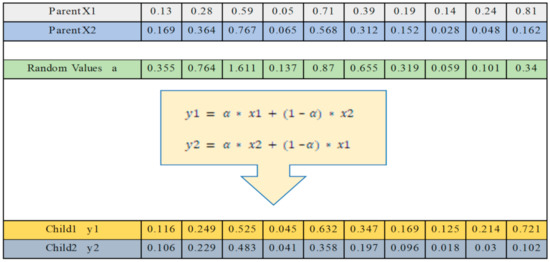
Figure 2.
Fitness-based crossover example.
Mutation Operator
The mutation gives a chance to the algorithm to escape from convergence to local optimality. As shown in Figure 3, after selecting a member for mutation, a number of the genes are selected and randomly changed based on the mutation steps.

Figure 3.
Swap mutation.
It should be noted that a solution representation method is used so that the solutions are continuously displayed between zero and one and are converted to continuous numbers through decoding. Hence, the algorithm only receives and processes numbers between zero and one so that the infeasible solutions are not generated. In addition, infeasible solutions are avoided by using the penalty function.
3.3.4. The MOPSO Metaheuristic Algorithm
The PSO algorithm was developed by Eberhart and Kennedy (1995) [47] inspired from the principles of the swarm intelligence. Each potential solution is considered as a particle and its status is recognized by its position and velocity. The position of the particle indicates a possible problem solution. Every particle moves towards the best position with a velocity that comprises the peculiarity of that particle’s best location visited too [48]. The MOPSO algorithm was introduced by Coello et al. (2004) [49]. MOPSO has been known by its superb performance and convergence. MOPSO, which is used to solve multi-objective optimization problems, is one of the most important intelligent optimization algorithms in the field of Swarm Intelligence.
3.3.5. The MOGWO Metaheuristic Algorithm
Mirjalili et al. (2014) introduced the MOGWO algorithm, afterwards, this algorithm was developed for solving multi-objective optimization problems [50,51]. MOGWO was inspired from the social behavior of gray wolves such as their hierarchical leadership and hunting mechanism in nature. According to Figure 4, the herd of gray wolves are grouped as alpha (α), beta (β), delta (δ) and omega (ω).
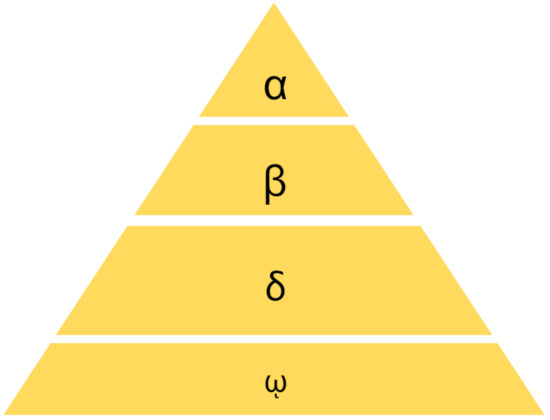
Figure 4.
The hierarchy of gray wolf society.
The first group, alpha (α), includes leaders who make decisions. The second group, beta (β), assists the leaders as advisors. The third group, delta (δ), does the duties and tasks such as hunting, scouting and guarding. The fourth group, omega (ω), takes the commands of the higher groups.
The most appropriate sets of solutions to a single-objective model are alpha (α), beta (β), delta (δ), and omega (ω), respectively.
3.4. Searching, Siege and Hunting Prey
Alpha set (the best group), beta set (the second group) and delta set (the third group) are considered to simulate wolf hunting. The following equations are used to determine the probability of prey locations:
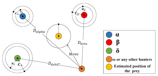
Figure 5.
Updating hunting position.
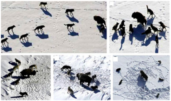
Figure 6.
Changing hunting position based on various alpha values.
A and C are determined using the below equations:
In which, a linearly decreases from 2 to 0 during each iteration, and r1 and r2 randomly change between 0 and 1 [51].
3.5. The Evaluation Metrics
It is important to evaluate the quality of a set of non-dominated solutions, since the incomparable and conflicting characteristics of some criteria make this procedure more complicated. Generally, the comparison of two Pareto approximations obtained by two unlike algorithms would not easy [52]. Nevertheless, the quality of the Pareto sets should be quantitatively assessed. Therefore, six metrics are applied in this study as follows.
3.5.1. CPU Computational Time
The less CPU computational time shows that the performance of the algorithm is better.
3.5.2. Mean Ideal Distance (MID)
The mean of closeness between the Pareto solutions and the ideal point (0,0,0) is measured by MID criterion [52]. For computing MID of maximizing objective function, the values of Pareto solutions are become inverse, and the ideal point is considered (0). The value of MID is calculated through the Equation (19):
where is the number of non-dominated set and . The lower value of , shows the better of performance for an algorithm.
3.5.3. Spread of Non-Dominance Solutions (SNS)
The SNS criterion [53], which is also known as the indicator of diversity, is calculated through the following equation:
The higher values of SNS, show the better solution quality, in other words, more diversity of solutions.
3.5.4. The Rate of Achievement to Two Objectives Simultaneously (RAS)
Another metric which is used for evaluation is known as RAS [53]. The value of this criterion is calculated using the following (and after calculating the best values of each target function):
where . The lower RAS value, the better solution quality assuming positive objective values.
3.5.5. Spacing (S)
The S performance metric, which is calculated through following equation, gives an indication of the evenness of solutions obtained from an algorithm [54,55]. A lower value of S shows a more uniform distribution of the obtained non-dominated solutions.
3.5.6. Diversification Matrix (DM)
This performance metric, which is calculated through following equation, gives an indication of diversity of solutions obtained from a given algorithm.
3.6. Parameter Tuning
The solution quality is influenced strongly by parameter setting. In this paper, the ranges of the parameters of the algorithms were identified through the literature survey [50,51,56,57,58,59]. Subsequently, the Taguchi method was applied to the sets of the parameters. The Taguchi method classifies the factors affecting the experimental results into uncontrollable (noise (N)) and controllable factors (signal (S)). Next, S/N is defined as the signal-to-noise ratio. The Taguchi method tunes the levels of factors at the maximum of the S/N ratio. Three different parameter levels were used in this study for the problems with 16, 40 and 75 activities, 2, 3 and 4 renewable resources and 2, 3 and 4 modes of executing activities for small, medium and large sizes respectively. These results are obtained using the Minitab software.
It is noteworthy that parameters of npop and NFE is considered equally for all algorithms because they have impressive effects on the solution values.
The defined parameter levels for the algorithms are presented in Table 2. The parameter levels of the NSGA-II, MOPSO, and MOGWO algorithms are obtained from the related studies [50,51,56,57,58,59].

Table 2.
Factors and factor levels of the algorithms.
Utility function includes three quantitative criteria and two qualitative criteria. The weight of 2 is allocated to the quantitative criteria, and the weight of 1 is assigned to the qualitative criteria, shown in the following equation [60]:
Determining the Normalized Weight Vector
The Shannon’s entropy parameter for the jth objective, denoted by , can be calculated by [61]:
denotes the jth objective function of the jth solution. represents the linear normalization of the jth objective for the jth solution, which is employed to determine the value of the Shannon’s entropy () of the jth objective. The number of objectives and solutions are displayed by m and , respectively. Eventually, the corresponding relative normalized weight for jth solution indicated by , is then obtained using Equation (27).
3.7. The WASPAS Method
The WASPAS method was first proposed by Zavadskas et al. (2012) [62]. The prioritization process of the solutions of the Pareto frontier is similar to the fuzzy WASPAS method which was proposed by Turskis et al. (2015) [63].
4. Results and Discussion
First, the proposed model was validated by solving a sample problem. Then, 30 problem instances were generated for the performance evaluation. The parameter amounts such as the earliest and latest start times were taken from the project scheduling library (PSPLIB) and the other specific parameters were generated by random number generator software based on a symmetry procedure (normal distribution). The parameters show in Table 3. Finally, a bridge construction project is considered as a case study.

Table 3.
The amounts of the parameters.
4.1. The Validation of the Proposed Model
In this step, one small size instance with 9 activities (including dummy start and finish activities), three renewable resources, three nonrenewable resources, and three activity execution modes are considered. The AON network, the earliest and latest start times and the due date of each activity are shown in Figure 7. The required amount of each renewable resource for each activity and activity duration in each mode and quality are represented in Table 4 and Table 5 respectively. The cost of one unit of renewable resource r and holding cost is shown in Table 6.
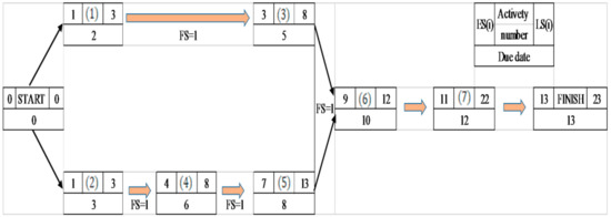
Figure 7.
Activity on node network.

Table 4.
Data of , and .

Table 5.
The amounts of renewable resource.

Table 6.
The amounts of costs.
This sample was solved with GAMS 24.1.2 software by augmented ε-constraint method (AEC). The thirtieth point of this frontier (cost = 126,116.5, makespan of project = 16, quality = 0.826) was selected, shown in Table 7, variables and take values properly according to duration and due date of each activity. The chart of resource allocation is shown in Figure 8.

Table 7.
and .
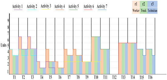
Figure 8.
Resource allocation chart.
The values of are given in Table 8.

Table 8.
Costs of renewable and non-renewable resources per unit of time.
Furthermore, this sample was solved by three meta-heuristic algorithms and the Pareto optimal frontiers are shown in Figure 9.
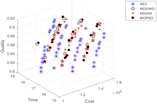
Figure 9.
Pareto frontiers of time-cost-quality by AEC and three metaheuristic solution methods.
Pareto frontier of time-cost objectives and cost-quality objectives are presented in Figure 10.
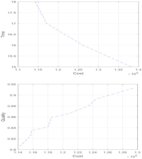
Figure 10.
Pareto frontier of time-cost objectives and cost-quality objectives.
As seen in Figure 10, the quality increases with cost. Additionally, project make-span increases with cost decrease. It is clear that higher project quality and shorter make-span will incur higher project costs.
4.2. Performance Analysis of the Algorithms
Thirty problem instances with various parameters were randomly generated, as shown in Table 9.

Table 9.
Data generation method.
The evolutionary algorithms were implemented in MATLAB software 2014 on a PC with corei30 USB and 10 GB of RAM. The results are presented in Table 10 and Table 11.

Table 10.
The data of three problem instances.

Table 11.
The average of six metrics for three proposed algorithms in small, medium, and large sizes.
As seen above, MOGWO outperforms the other algorithms based on the Diversity, SNS, MID, and RAS indices. On the other hand, NSGA-II has a better performance than the other algorithms in terms of Spacing. Finally, MOPSO is better than other algorithms based on time.
It’s notable, if the outputs of algorithms (the value of metrics) don’t be normal, it should be normalized through Box–Cox transforming and become symmetry.
The statistical analysis of the model was implemented in the form of analysis of variance (ANOVA) for all metrics. Figure 11 shows the means plot of the different metrics in numerical example (at the 95% confidence level).
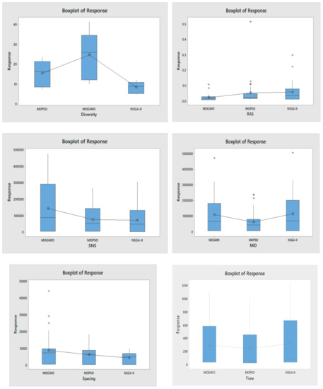
Figure 11.
The plot of all metrics for all the algorithms.
Comparison of MOGWO and NSGA-II show that there are significant differences between two algorithms based on Diversity, RAS, SNS, and Spacing, MOGWO outperforms based on Diversity, SNS and RAS, and NSGA-II has a better performance based on Spacing. There are no significant differences in term of MID and CPU time.
Comparison of MOGWO and MOPSO show that MOGWO outperforms based on Diversity, RAS, and SNS. There are no significant differences in term of other indices.
The results also indicate that NSGA-II has better performance in term of Spacing. However, MOPSO outperforms based on Diversity. There are no significant differences in term of other indices.
MOPSO is better than MOGWO and NSGA-II in term of the CPU time.
4.3. Case Study
Building a bridge is a complex undertaking requiring knowledge and expertise. Numerous variables, including engineering constraints, costs, time, and quality impacts come into play when deciding which construction method to use and bridge type to build. In recent years, several bridges of different types have been under construction on the Shiraz–Isfahan freeway in Iran. In this paper, the concrete bridge of the Shiraz–Isfahan freeway, which is part of the Shiraz–Isfahan freeway project, is considered as a case study for model evaluation. This project consists of 88 activities with an estimated duration of 36 months and a total budget of 26 billion Tomans (6.5 million Dollars). Seventeen renewable resources (worker, workmanship, formwork worker, ironworker, rebar worker, engineer, tower crane, pile driver, power shovel, concrete mixer, concrete pump, truck, road marking machine, primer spraying machine, roller machine, beam launcher, formwork set) and eight non-renewable resources (concrete, lean concrete, paint, asphalt, tar, bituminous waterproofing, rebar and prefabricated steel) are required for accomplishing the project. The implementation phase of this project has initiated in July 2015. After solving the proposed model by information of bridge construction case, the results are presented in the next parts.
4.3.1. 3-Dimensional Objective Space
The Pareto set was first generated for the problem containing three objective functions of time, cost, and quality. Figure 12 shows the set of 3D Pareto points produced by running.
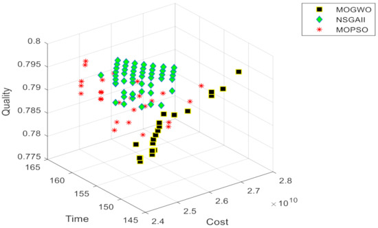
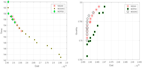
Figure 12.
Pareto sets of solutions for the three-criteria and two-criteria multi-objective optimization problem.
Comparison with the case study where the NPV is calculated at the completion of the activity.
As shown in Figure 13, the cost objective function has a lower value when NPV is calculated at the end of each activity. Therefore, calculating NPV at the end of each activity leads to not considering some amounts of costs, and the cost overrun is occurred, which is typical in most projects.
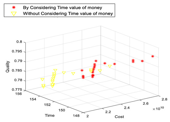
Figure 13.
The comparison with the case when the NPV is calculated at the end of each activity.
4.3.2. Finding the Best Solution through MCDM Methods
The Pareto sets of solutions for three meta-heuristic algorithms are presented in Figure 12. The best Pareto solution is selected using the MCDM method; First, the criteria (objective functions) are weighted using the Shannon’s entropy technique, subsequently, the alternatives (the solutions) are ranked using the WASPAS method. The weight of each criterion is presented in Table 12. Among the Pareto solutions, the 96th solution (cost 25466429315, time 153, quality 0.79886) has the highest utility score.

Table 12.
The weight of criteria.
In addition, the Gantt chart related to the best solution is presented in Figure 14.
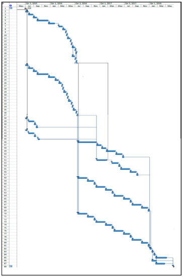
Figure 14.
The corresponding Gantt chart with the best solution of Pareto frontier.
4.4. Discussion
Considering the small-sized problems, the results of the three metaheuristic algorithms of NSGA-II, MOGWO, MOPSO, and the results obtained from GAMS software were compared in order to validate these metaheuristic algorithms. Due to the NP-Hardness of the proposed model, the exact methods and GAMS optimization software are not able to find the optimal solutions for the large-sized problems. Hence, these three metaheuristic algorithms were employed using the MATLAB software. Thirty small, medium and large size test problems were designed, and six indices of time, DM, RAS, MID, Spacing, and SNS were considered for performance evaluation. The results showed that the MOGWO algorithm has better performance than the other two algorithms.
Additionally, the impact of considering the time value of money was evaluated. As shown in Figure 13, the cost objective function is greater when NPV is calculated by executing activities in each period. Therefore, calculating NPV at the end of each activity leads to not considering some amounts of costs and the cost overrun which is typical in most projects. In this case study, if we do not consider the time value of money there is about 22 percent cost overrun in project. Therefore, it is very important to consider the time value of money and also the other indirect cost of the project in order to prevent cost overrun.
Figure 12 shows that cost objective function and time and quality objective functions conflict with each other so that by increasing project costs, the duration of the project decreases, and the total quality of the project increases. As can be seen in Figure 13, in the interval (149 weeks,154 weeks) period of time that project is completed, by increasing 0.4 to 1 percent in the total cost of the project can reduce 1 period of time of project make-span. Additionally, it can reduce 19 periods of time by increasing 16 percent in project total cost. Regarding the quality objective function, it can be said that with 8 percent increasing in project total cost, 1.3 units can be added to the overall quality level of the project.
After ranking the Pareto Set of solutions using the MCDM method, the best solution is selected regarding the project decision-makers’ policies and preference. The corresponding Gantt chart of this solution is represented in Figure 14. According to the Gantt chart, the project was started in July 2015 and was completed in July 2018, with a total duration of 154 weeks. However, the total project duration of 153 weeks was obtained based on the best Pareto solution that indicates the efficient performance of the proposed methodology.
5. Conclusions
In this paper, a multi-objective mathematical programming model was presented for resource constraint project scheduling problem (RCPSP) with the aim of time, cost, and quality trade-off considering the time value of money. Additionally, the proposed model was implemented on a real case study of a bridge construction project with 88 activities and solved by three different metaheuristic algorithms named NSGA-II, MOPSO, and MOGWO. The best Pareto solution was selected using the MCDM techniques including the Shannon’s entropy technique and WASPAS method.
It should be noted that the value of the cost objective function is greater when the net present value (NPV) is calculated based on each unit of time period. However, calculating NPV based on the finish times of activities leads to not considering the real amount of costs and results in cost overrun. In addition, the findings of this study showed that the objective functions of the TCQ trade-off problem are conflicting. In other words, improving the value of one objective function leads to deteriorating the values of the other objective functions. Moreover, the results demonstrated the efficiency of the metaheuristic algorithms in solving the proposed multi-objective optimization model. However, the MOGWO algorithm outperforms the others in terms of the six well-known metrics including time, MID, SNS, RAS, Spacing, and DM.
The limitation of research that can be concisely counted, are as follows: Gathering input data of the real construction project with 88 activities was time-consuming and challenging. In addition, due to the NP-Hardness of the problem in hand, the CPU run time for the problem instances (especially large size problems) was quite long. As suggestions for future research, it is recommended to implement the proposed model on large-sized projects and analyze the results. Additionally, the environmental impacts of project activities and social aspects of the project can be considered as other objective functions. Moreover, the fuzzy set theory may be applied to deal with the uncertain parameters of projects. Furthermore, other MCDM methods may be applied to weight the objective functions and choose the best solution.
Author Contributions
Conceptualization, O.K.; methodology, O.K. and A.H.; software, A.H.; validation, M.K.; formal analysis, O.K.; investigation, O.K.; resources, M.K.; data curation, O.K.; writing—original draft preparation, O.K., A.H. and M.K.; writing—review and editing, M.K. and J.A.; funding acquisition, J.A. and M.P.; final revision and layout, J.A. and M.P. All authors have read and agreed to the published version of the manuscript.
Funding
This research received no external funding.
Institutional Review Board Statement
Not applicable.
Informed Consent Statement
Not applicable.
Data Availability Statement
Data is available upon request.
Conflicts of Interest
The authors declare no conflict of interest.
References
- Nagyová, A.; Pačaiová, H.; Markulik, Š.; Turisová, R.; Kozel, R.; Džugan, J. Design of a Model for Risk Reduction in Project Management in Small and Medium-Sized Enterprises. Symmetry 2021, 13, 763. [Google Scholar] [CrossRef]
- Kaveh, A.; Vazirinia, Y. Chaotic Vibrating Particles System for Resource-Constrained Project Scheduling Problem. Sci. Iran. 2020, 27, 1826–1842. [Google Scholar] [CrossRef] [Green Version]
- Banihashemi, S.A.; Khalilzadeh, M.; Antucheviciene, J.; Šaparauskas, J. Trading off Time–Cost–Quality in Construction Project Scheduling Problems with Fuzzy SWARA–TOPSIS Approach. Buildings 2021, 11, 387. [Google Scholar] [CrossRef]
- Sonmez, R.; Bettemir, Ö.H. A hybrid genetic algorithm for the discrete time–cost trade-off problem. Expert Syst. Appl. 2012, 39, 11428–11434. [Google Scholar] [CrossRef] [Green Version]
- Monghasemi, S.; Nikoo, M.R.; Fasaee, M.A.K.; Adamowski, J. A novel multi criteria decision making model for optimizing time–cost–quality trade-off problems in construction projects. Expert Syst. Appl. 2015, 42, 3089–3104. [Google Scholar] [CrossRef]
- Afshar, A.; Ziaraty, A.K.; Kaveh, A.; Sharifi, F. Nondominated archiving multicolony ant algorithm in time–cost trade-off optimization. J. Constr. Eng. Manag. 2009, 135, 668–674. [Google Scholar] [CrossRef]
- Mungle, S.; Benyoucef, L.; Son, Y.J.; Tiwari, M.K. A fuzzy clustering-based genetic algorithm approach for time–cost–quality trade-off problems: A case study of highway construction project. Eng. Appl. Artif. Intell. 2013, 26, 1953–1966. [Google Scholar] [CrossRef]
- Afruzi, E.N.; Najafi, A.A.; Roghanian, E.; Mazinani, M. A multi-objective imperialist competitive algorithm for solving discrete time, cost and quality trade-off problems with mode-identity and resource-constrained situations. Comput. Oper. Res. 2014, 50, 80–96. [Google Scholar] [CrossRef]
- Tavana, M.; Abtahi, A.R.; Khalili-Damghani, K. A new multi-objective multi-mode model for solving preemptive time–cost–quality trade-off project scheduling problems. Expert Syst. Appl. 2014, 41, 1830–1846. [Google Scholar] [CrossRef]
- Zareei, M.; Hassan-Pour, H.A. A multi-objective resource-constrained optimization of time-cost trade-off problems in scheduling project. Iran. J. Manag. Stud. 2015, 8, 653–685. [Google Scholar]
- Saif, A.; Abbas, S.; Fayed, Z. The PDBO algorithm for discrete time, cost and quality trade-off in software projects with expressing quality by defects. Procedia Comput. Sci. 2015, 65, 930–939. [Google Scholar] [CrossRef] [Green Version]
- Fu, F.; Zhang, T. A new model for solving time-cost-quality trade-off problems in construction. PLoS ONE 2016, 11, e0167142. [Google Scholar] [CrossRef] [PubMed] [Green Version]
- Hosseini, S.A.; Akbarpour, A.; Ahmadi, H.; Aminnejad, B. Balance of cost, time, and quality related to construction projects regarding the reinforced concrete of underground structures using a meta-heuristic algorithm. Arch. Civ. Eng. 2017, 63, 103–121. [Google Scholar] [CrossRef] [Green Version]
- Orm, M.B.; Jeunet, J. Time Cost Quality Trade-off Problems: A survey exploring the assessment of quality. Comput. Ind. Eng. 2018, 118, 319–328. [Google Scholar] [CrossRef]
- Geshniani, Y.V.; Kamranrad, R.; Emam, I. A multi-objective scheduling payment pattern for project cash flow by considering resource constraints (a case study in power transfer system). Int. J. Ind. Syst. Eng. 2020, 35, 299. [Google Scholar] [CrossRef]
- Mehrdad, P. A new method for scheduling resource constrained projects using a heuristic. Int. J. Adv. Heuristic Meta-Heuristic Algorithms 2020, 1, 77–104. [Google Scholar]
- Mahmoudi, A.; Javed, S.A. Project scheduling by incorporating potential quality loss cost in time-cost tradeoff problems: The revised KKH model. J. Model. Manag. 2020, 15, 1187–1204. [Google Scholar] [CrossRef]
- Sharma, K.; Trivedi, M.K. Latin hypercube sampling-based NSGA-III optimization model for multimode resource constrained time–cost–quality–safety trade-off in construction projects. Int. J. Constr. Manag. 2020, 1–11. [Google Scholar] [CrossRef]
- Moghadam, E.K.; Sharifi, M.; Rafiee, S.; Chang, Y.K. Time–Cost–Quality Trade-Off in a Broiler Production Project Using Meta-Heuristic Algorithms: A Case Study. Agriculture 2020, 10, 3. [Google Scholar] [CrossRef] [Green Version]
- Jeunet, J.; Orm, M.B. Optimizing temporary work and overtime in the Time Cost Quality Trade-off Problem. Eur. J. Oper. Res. 2020, 284, 743–761. [Google Scholar] [CrossRef]
- Keshavarz, E.; Shoul, A. Project Time-Cost-Quality Trade-off Problem: A Novel Approach Based on Fuzzy Decision Making. Int. J. Uncertain. Fuzziness Knowl.-Based Syst. 2020, 28, 545–567. [Google Scholar] [CrossRef]
- Banihashemi, S.A.; Khalilzadeh, M. Time-cost-quality-environmental impact trade-off resource-constrained project scheduling problem with DEA approach. Eng. Constr. Archit. Manag. 2021, 28, 1979–2004. [Google Scholar] [CrossRef]
- Mao, X.; Li, J.; Guo, H.; Wu, X. Research on Collaborative Planning and Symmetric Scheduling for Parallel Shipbuilding Projects in the Open Distributed Manufacturing Environment. Symmetry 2020, 12, 161. [Google Scholar] [CrossRef] [Green Version]
- Panwar, A.; Jha, K.N. Integrating quality and safety in construction scheduling time-cost trade-off model. J. Constr. Eng. Manag. 2021, 147, 04020160. [Google Scholar] [CrossRef]
- Hosseinzadeh, F.; Paryzad, B.; Pour, N.S.; Najafi, E. Fuzzy combinatorial optimization in four-dimensional tradeoff problem of cost-time-quality-risk in one dimension and in the second dimension of risk context in ambiguous mode. Eng. Comput. 2020, 37, 1967–1991. [Google Scholar] [CrossRef]
- Luong, D.L.; Tran, D.H.; Nguyen, P.T. Optimizing multi-mode time-cost-quality trade-off of construction project using opposition multiple objective difference evolution. Int. J. Constr. Manag. 2021, 21, 271–283. [Google Scholar] [CrossRef]
- Hamta, N.; Ehsanifar, M.; Sarikhani, J. Presenting a goal programming model in the time-cost-quality trade-off. Int. J. Constr. Manag. 2021, 21, 1–11. [Google Scholar] [CrossRef]
- Nguyen, D.T.; Doan, D.T.V.; Tran, N.N.C.; Tran, D.H. A novel multiple objective whale optimization for time-cost-quality tradeoff in non-unit repetitive projects. Int. J. Constr. Manag. 2021, 1–12. [Google Scholar] [CrossRef]
- Huynh, V.H.; Nguyen, T.H.; Pham, H.C.; Huynh, T.M.D.; Nguyen, T.C.; Tran, D.H. Multiple Objective Social Group Optimization for Time–Cost–Quality–Carbon Dioxide in Generalized Construction Projects. Int. J. Civ. Eng. 2021, 19, 805–822. [Google Scholar] [CrossRef]
- Banihashemi, S.A.; Khalilzadeh, M.; Zavadskas, E.K.; Antucheviciene, J. Investigating the Environmental Impacts of Construction Projects in Time-Cost Trade-Off Project Scheduling Problems with CoCoSo Multi-Criteria Decision-Making Method. Sustainability 2021, 13, 10922. [Google Scholar] [CrossRef]
- Liu, S.S.; Budiwirawan, A.; Arifin, M.F.A.; Chen, W.T.; Huang, Y.H. Optimization Model for the Pavement Pothole Repair Problem Considering Consumable Resources. Symmetry 2021, 13, 364. [Google Scholar] [CrossRef]
- Tiwari, V.; Patterson, J.H.; Mabert, V.A. Scheduling projects with heterogeneous resources to meet time and quality objectives. Eur. J. Oper. Res. 2009, 193, 780–790. [Google Scholar] [CrossRef]
- Kim, J.; Kang, C.; Hwang, I. A practical approach to project scheduling: Considering the potential quality loss cost in the time–cost tradeoff problem. Int. J. Proj. Manag. 2012, 30, 264–272. [Google Scholar] [CrossRef]
- Wood, D.A. Gas and oil project time-cost-quality tradeoff: Integrated stochastic and fuzzy multi-objective optimization applying a memetic, nondominated, sorting algorithm. J. Nat. Gas Sci. Eng. 2017, 45, 143–164. [Google Scholar] [CrossRef]
- Dodin, B.; Elimam, A.A. Integrated project scheduling and material planning with variable activity duration and rewards. Iie Trans. 2001, 33, 1005–1018. [Google Scholar] [CrossRef]
- Seyfi, M.; Tavakoli, M.R. A new bi-objective model for a multi-mode resource-constrained project scheduling problem with discounted cash flows and four payment models. Int. J. Eng. 2008, 21, 347–360. [Google Scholar]
- Khoshjahan, Y.; Najafi, A.A.; Afshar-Nadjafi, B. Resource constrained project scheduling problem with discounted earliness–tardiness penalties: Mathematical modeling and solving procedure. Comput. Ind. Eng. 2013, 66, 293–300. [Google Scholar] [CrossRef]
- Balali, A.; Valipour, A.; Antucheviciene, J.; Šaparauskas, J. Improving the results of the earned value management technique using artificial neural networks in construction projects. Symmetry 2020, 12, 1745. [Google Scholar] [CrossRef]
- Deb, K. Multi-Objective Optimization Using Evolutionary Algorithms; John Wiley & Sons: Hoboken, NJ, USA, 2001. [Google Scholar]
- Punnathanam, V.; Sivadurgaprasad, C.; Kotecha, P. Multi-objective Optimal Integration of Biorefineries using NSGA-II and MOGWO. In Proceedings of the 2016 International Conference on Electrical, Electronics, and Optimization Techniques (ICEEOT), Chennai, India, 3–5 March 2016; pp. 3970–3975. [Google Scholar]
- Agrebi, I.; Jemmali, M.; Alquhayz, H.; Ladhari, T. Metaheuristic algorithms for the two-machine flowshop scheduling problem with release dates and blocking constraint. J. Chin. Inst. Eng. Trans. Chin. Inst. Eng. Ser. A 2021, 44, 573–582. [Google Scholar] [CrossRef]
- Goodarzian, F.; Kumar, V.; Ghasemi, P. A set of efficient heuristics and meta-heuristics to solve a multi-objective pharmaceutical supply chain network. Comput. Ind. Eng. 2021, 158, 107389. [Google Scholar] [CrossRef]
- Mavrotas, G. Effective implementation of the ε-constraint method in multi-objective mathematical programming problems. Appl. Math. Comput. 2009, 213, 455–465. [Google Scholar] [CrossRef]
- Amirian, H.; Sahraeian, R. Augmented ε-constraint method in multi-objective flowshop problem with past sequence set-up times and a modified learning effect. Int. J. Prod. Res. 2015, 53, 5962–5976. [Google Scholar] [CrossRef]
- Deb, K.; Pratap, A.; Agarwal, S.; Meyarivan, T.A.M.T. A fast and elitist multiobjective genetic algorithm: NSGA-II. IEEE Trans. Evol. Comput. 2002, 6, 182–197. [Google Scholar] [CrossRef] [Green Version]
- Li, K.; Pan, L.; Xue, W.; Jiang, H.; Mao, H. Multi-objective optimization for energy performance improvement of residential buildings: A comparative study. Energies 2017, 10, 245. [Google Scholar] [CrossRef] [Green Version]
- Eberhart, R.; Kennedy, J. A new optimizer using particle swarm theory. In MHS’95, Proceedings of the Sixth International Symposium on Micro Machine and Human Science, IEEE, Nagoya, Japan, 4–6 October 1995; IEEE: New York, NY, USA, 1995; pp. 39–43. [Google Scholar]
- Zhang, H.; Xing, F. Fuzzy-multi-objective particle swarm optimization for time–cost–quality tradeoff in construction. Autom. Constr. 2010, 19, 1067–1075. [Google Scholar] [CrossRef]
- Coello, C.A.C.; Pulido, G.T.; Lechuga, M.S. Handling multiple objectives with particle swarm optimization. IEEE Trans. Evol. Comput. 2010, 8, 256–279. [Google Scholar] [CrossRef]
- Mirjalili, S.; Mirjalili, S.M.; Lewis, A. Grey wolf optimizer. Adv. Eng. Softw. 2014, 69, 46–61. [Google Scholar] [CrossRef] [Green Version]
- Mirjalili, S.; Saremi, S.; Mirjalili, S.M.; Coelho, L.D.S. Multi-objective grey wolf optimizer: A novel algorithm for multi-criterion optimization. Expert Syst. Appl. 2016, 47, 106–119. [Google Scholar] [CrossRef]
- Behnamian, J.; Ghomi, S.F.; Zandieh, M. A multi-phase covering Pareto-optimal front method to multi-objective scheduling in a realistic hybrid flowshop using a hybrid metaheuristic. Expert Syst. Appl. 2009, 36, 11057–11069. [Google Scholar] [CrossRef]
- Jolai, F.; Asefi, H.; Rabiee, M.; Ramezani, P. Bi-objective simulated annealing approaches for no-wait two-stage flexible flow shop scheduling problem. Sci. Iran. 2013, 20, 861–872. [Google Scholar]
- Schott, J.R. Fault Tolerant Design Using Single and Multicriteria Genetic Algorithm Optimization (No. AFIT/CI/CIA-95-039); Air Force Institute of Tech: Dayton, OH, USA, 1995. [Google Scholar]
- Kaveh, A.; Mahdavi, V.R. Multi-objective colliding bodies optimization algorithm for design of trusses. J. Comput. Des. Eng. 2019, 6, 49–59. [Google Scholar] [CrossRef]
- Rabiee, M.; Zandieh, M.; Ramezani, P. Bi-objective partial flexible job shop scheduling problem: NSGA-II, NRGA, MOGA and PAES approaches. Int. J. Prod. Res. 2012, 50, 7327–7342. [Google Scholar] [CrossRef]
- Tabrizi, B.H.; Ghaderi, S.F. A robust bi-objective model for concurrent planning of project scheduling and material procurement. Comput. Ind. Eng. 2016, 98, 11–29. [Google Scholar] [CrossRef]
- Habibi, F.; Barzinpour, F.; Sadjadi, S.J. A mathematical model for project scheduling and material ordering problem with sustainability considerations: A case study in Iran. Comput. Ind. Eng. 2019, 128, 690–710. [Google Scholar] [CrossRef]
- Jafarian, A.; Rabiee, M.; Tavana, M. A novel multi-objective co-evolutionary approach for supply chain gap analysis with consideration of uncertainties. Int. J. Prod. Econ. 2020, 228, 107852. [Google Scholar] [CrossRef]
- Asefi, H.; Jolai, F.; Rabiee, M.; Araghi, M.T. A hybrid NSGA-II and VNS for solving a bi-objective no-wait flexible flowshop scheduling problem. Int. J. Adv. Manuf. Technol. 2014, 75, 1017–1033. [Google Scholar] [CrossRef]
- Khorasani, G.; Mirmohammadi, F.; Motamed, H.; Fereidoon, M.; Tatari, A.; Verki, M.R.M.; Khorasani, M.; Fazelpour, S. Application of multi criteria decision making tools in road safety performance indicators and determine appropriate method with average concept. Int. J. Innov. Technol. Explor. Eng. 2013, 3, 173–177. [Google Scholar]
- Zavadskas, E.K.; Turskis, Z.; Antucheviciene, J.; Zakarevicius, A. Optimization of Weighted Aggregated Sum Product Assessment. Elektron. Elektrotechnika 2012, 122, 3–6. [Google Scholar] [CrossRef]
- Turskis, Z.; Zavadskas, E.K.; Antucheviciene, J.; Kosareva, N. A hybrid model based on fuzzy AHP and fuzzy WASPAS for construction site selection. Int. J. Comput. Commun. Control. 2015, 10, 873–888. [Google Scholar] [CrossRef]
- Paryzad, B.; Pour, N.S. Time-cost-quality-risk trade-off in GIGA projects using specific techniques of hunting dolphins. Int. J. Ind. Syst. Eng. 2016, 22, 484–499. [Google Scholar] [CrossRef]
Publisher’s Note: MDPI stays neutral with regard to jurisdictional claims in published maps and institutional affiliations. |
© 2021 by the authors. Licensee MDPI, Basel, Switzerland. This article is an open access article distributed under the terms and conditions of the Creative Commons Attribution (CC BY) license (https://creativecommons.org/licenses/by/4.0/).