On the Hierarchical Bernoulli Mixture Model Using Bayesian Hamiltonian Monte Carlo

Abstract

The model developed considers the uniqueness of a data-driven binary response (indicated by 0 and 1) identified as having a Bernoulli distribution with finite mixture components. In social science applications, Bernoulli’s constructs a hierarchical structure data. This study introduces the Hierarchical Bernoulli mixture model (Hibermimo), a new analytical model that combines the Bernoulli mixture with hierarchical structure data. The proposed approach uses a Hamiltonian Monte Carlo algorithm with a No-U-Turn Sampler (HMC/NUTS). The study has performed a compatible syntax program computation utilizing the HMC/NUTS to analyze the Bayesian Bernoulli mixture aggregate regression model (BBMARM) and Hibermimo. In the model estimation, Hibermimo yielded a result of ~90% compliance with the modeling of each district and a small Widely Applicable Information Criteria (WAIC) value.

1. Introduction

The Bernoulli distribution is frequently used for data mining, particularly for text analysis, and it has been improved into a mixture model called the Bernoulli Mixture Model (BMM) [1]. The BMM evolves on the basis of the mixture distribution, representing data patterns from a data-driven analysis perspective [2]. The expansion of BMM was discussed by Grim et al. [3], González et al. [4], Juan and Vidal [5,6], Patrikainen and Manilla [7], Bouguila [8], Zhu et al. [9], Sun et al. [10], Tikka et al. [11], Myllykangas et al. [12], and Saeed et al. [13]. This research proposes a model by considering the uniqueness of binary response data (0 and 1) identified as having a Bernoulli distribution with finite mixture components that can be applied in the area of social science.

The uniqueness of the data-driven distribution of a Bernoulli mixture when applied to social science concentrates on tracing the relationships between the units of observation and the social environment. Social science concepts emphasize that units are correlated with social communities. The units are affected by the characteristics of the social environment in which they are located [14]. In general, social units and districts are united in a hierarchical system to build a hierarchical data structure. The hierarchical data structure implies that the unit-level has a nested structure or is clustered at the district level. The information at each level in a hierarchical data structure must be statistically analyzed simultaneously [15,16]. The hierarchical model aims to measure the response variables explained by the explanatory variables at each level of the hierarchical data structure [17]. Additionally, Ringdal [18], by accounting for individual membership in the area/environment, aimed to make the expected inference.

This study develops the Hierarchical Bernoulli mixture model (Hibermimo). This model combines the concept of a hierarchical structure with the BMM, considering the uniqueness of data. In Hibermimo, the binary or dichotomous response variable must use a link function in the estimation process. We fit the logit link function in a Level 1 model, linking the linear predictor and the Bernoulli mixture distribution. One study using BMM with this link function has been performed by Suryaningtyas et al. [19], which discussed scholarship classifications using Bayesian MCMC.

Hibermimo analysis performs well in complex models. Parameter estimation for Hibermimo using the classical (frequentist) approach is insufficient. Recently, there has been strong interest in the Hamiltonian Monte Carlo algorithm with No-U-Turn Sampler (HMC/NUTS) for implementing the proposed model. Here, we provide a simple syntax for the computation of the model using the Stan program. Stan, a probabilistic programming language for specifying statistical models, allows full Bayesian inference using the HMC/NUTS strategy, an adaptive form of sampling [20]. This research aims to study the theoretical and computational estimators of the Hibermimo two-level parameters with an approach using the HMC/NUTS algorithm. Furthermore, we also empirically studied the application of Hibermimo in social science in the case of Bidikmisi in East Java Province. Analytical Hibermimo compares its effectiveness with the Bayesian Bernoulli mixture aggregate regression model (BBMARM) using WAIC.

The rest of the study is structured as follows. Section 2 describes the Bernoulli Mixture Model and the likelihood. We provide a directed acyclic graph (DAG) as a graphical model to illustrate the relationships between the data used with parameters and prior distributions at each hierarchy level. In addition, we present a prior assumption at the micro-level and macro-level and the form of the joint posterior distribution. The parameter estimation method of the Hierarchical Bernoulli Mixture Model using the Hamiltonian Monte Carlo algorithm is given in Section 3. This section also applies models to the unique binary responses of the Bidikmisi scholarship data (0 and 1), identified as having a Bernoulli distribution with finite mixture components. Section 4 discusses the performance of the best models, and Section 5 presents the conclusions and addresses future research in Hibermimo.

2. Materials and Methods

2.1. Bernoulli Mixture Model

If a random sample $Y$ derived from unit $i$ at level $j$ includes binary response data (0 and 1), it could be identified as having a Bernoulli mixture distribution. The vector $\mathbf{y}={\left[\begin{array}{cccc}{y}_{1j}& y_{2j}& \cdots & y_{nm}\end{array}\right]}^T$, $i=1,2,\dots ,n$, $j=1,2,\dots ,m$ can contain a finite number of $C$ mixed groups with the proportion $\mathsf{\pi }=\left({\pi }_1,{\pi }_2,\dots ,{\pi }_C\right)$ with ${\sum }_c^C{\pi }_c=1$. The density functions for the finite mixture model (FMM) of $Y$ were presented by McLachlan and Peel [21]. The finite Bernoulli mixture model (FBMM) for the $𝒸$ number of components can be rewritten as:

$$\begin{array}{cc}\hfill p\left(y_{ij}|\mathsf{\omega }\right)& ={\displaystyle \sum _{c=1}^C}{\pi }_c{p}_c\left(y_{ij}|{\theta }_{ijc}\right)\hfill \\ & ={\displaystyle \sum _{c=1}^C}{\pi }_c{\theta }_{ijc}{}^{y_{ij}}{\left(1-{\theta }_{ijc}\right)}^{1-y_{ij}},\hfill \end{array}$$

(1)

where $\mathsf{\omega }=\left(\mathsf{\pi },\mathsf{\theta }\right)$, $\mathsf{\pi }=\left({\pi }_1,{\pi }_2,\dots ,{\pi }_C\right)$, and $\mathsf{\theta }=\left({\theta }_{ij1},{\theta }_{ij2},\dots ,{\theta }_{ijC}\right)$. ${\theta }_{ijc}$ is the parameter distribution of the Bernoulli mixture with the probability of success of the $i$-th unit at the $j$-th level of the $c$-th mixture component. Identification of each data unit $i$ to be classified as a member of the mixture components in BMM as in (1) must use a latent variable, $z$. The working scenario is that there is an indicator vector ${\mathbf{z}}_i$ which can classify $y_{ij}$ into $𝒸$ different numbers of mixture components. This latent variable, therefore, would consist of defined vector latent membership. The complete likelihood of BMM would be as shown in Equation (2).

$$p_C\left(\mathbf{y},\mathbf{z}|\mathsf{\omega }\right)={\displaystyle \prod _{j=1}^m}{\displaystyle \prod _{i=1}^n}{\displaystyle \prod _{c=1}^C}{\left[{\pi }_c{\theta }_{ijc}{}^{y_{ij}}{\left(1-{\theta }_{ijc}\right)}^{1-y_{ij}}\right]}^{z_{ic}},$$

(2)

to estimate the model, we can then obtain the marginal density function of $p\left(\mathbf{z}|\mathsf{\pi }\right)$ and $p\left(\mathbf{y}|\mathbf{z},\mathsf{\theta }\right)$ from the decomposition of the likelihood function in Equation (2).

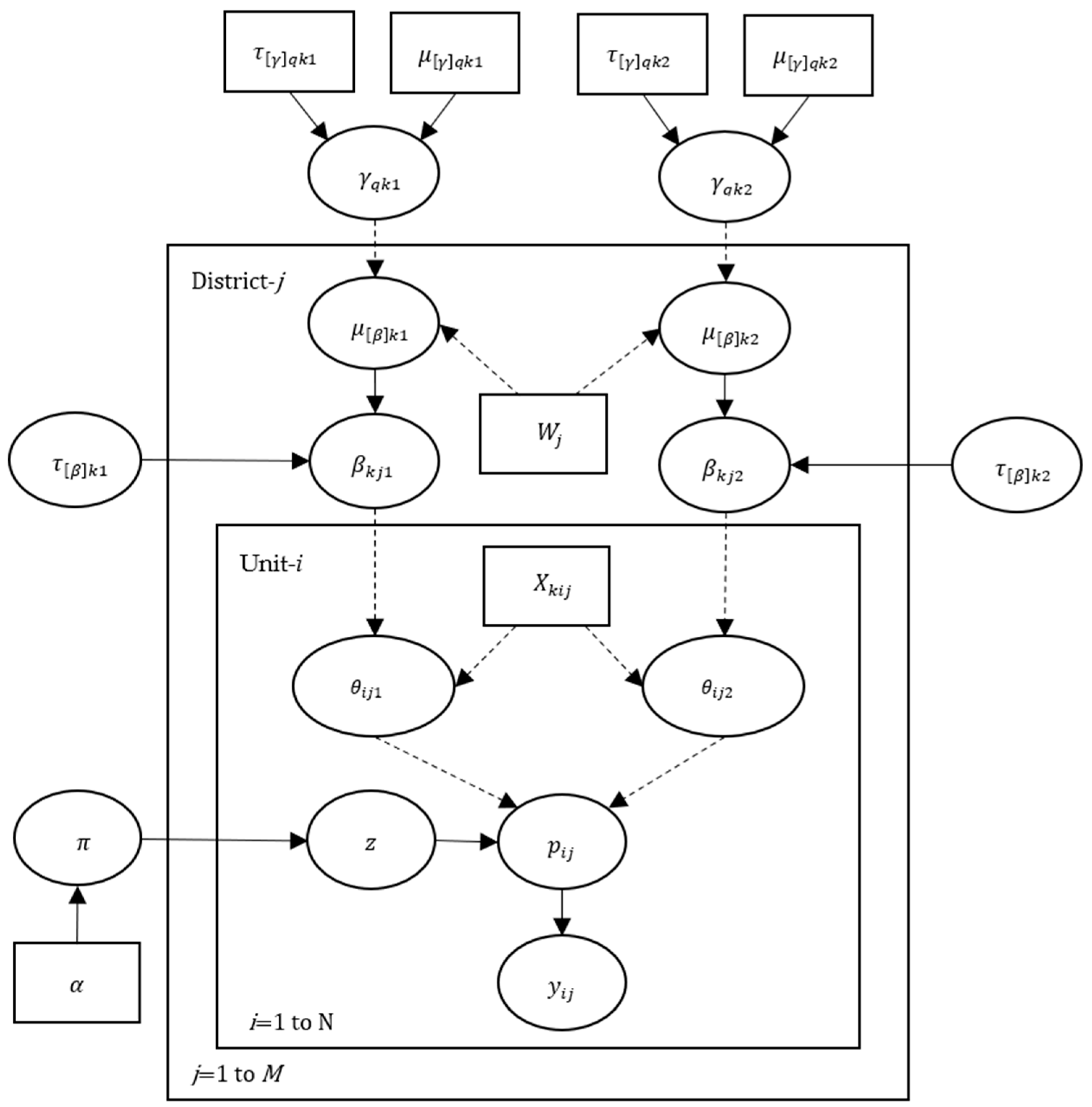
2.2. Directed Acyclic Graph of Hibermimo

Directed acyclic graph (DAG) is a graphical model representing the relationships between the data used and parameters, and the prior distributions at each hierarchical level in the analysis using the Bayesian approach [22]. The Hierarchical Bernoulli mixture model (Hibermimo) DAG using the Bayesian Hamiltonian Monte Carlo algorithm shows the position of the hyperprior hierarchy level and the relationships among the prior distributions for the micro- and macro-model parameters independently at each level. The DAG of the two-level Hibermimo is presented in Figure 1.

The notation $y_{ij}$ in Figure 1 is defined as the binary response of the finite Bernoulli mixture distribution (for every unit $i$ of the observation data for district $j$) with two components, i.e., Bernoulli Component 1 $\left({\theta }_{ij1}\right)$ and Bernoulli Component 2 $\left({\theta }_{ij2}\right)$. The indicator vector $\mathbf{z}$ classifies the data in the mixture according to the component criteria. The proportion of $\mathsf{\pi }$ is set as Dirichlet distribution, and the hyper-parameters of the Dirichlet prior are expressed as $\alpha$. Each Bernoulli mixture component, ${\theta }_{ij1}$ and ${\theta }_{ij2}$, is supposed to be influenced by $X_{kij}$ at the micro-level and by covariate $W_j$ at the macro-level. Furthermore, ${\gamma }_{qk1}$ and ${\gamma }_{qk2}$ are parameters at the macro-level with a normal conjugate prior distribution. These two parameters will build a linear combination of covariates at the macro-level $W_j$, represented as ${\mu }_{\left[\beta \right]k1}$ and ${\mu }_{\left[\beta \right]k2}$. This can explain the variability of the parameters at the micro-level, ${\beta }_{kj1}$ and ${\beta }_{kj2}$.

2.3. Prior Distribution of Hibermimo

The DAG of the two-level Hibermimo in Figure 1 shows the relationships between the distribution of the prior parameters at the micro- and macro-levels, which are independent to avoid the high collinearity between the predictor variables in two-level Hibermimo modeling [23,24]. At the micro-level and macro-level, the prior distribution integrates the conjugate, informative, and pseudo-informative priors [23].

The following prior assumptions are imposed:

$${\beta }_{kjc}\sim N\left({\mu }_{\left[\beta \right]kc},{\sigma }_{\left[\beta \right]kc}^2\right),$$

(3)

$${\gamma }_{qkc}\sim N\left({\mu }_{\left[\gamma \right]qkc},{\sigma }_{\left[\gamma \right]qkc}^2\right),$$

(4)

$${\tau }_{\left[\beta \right]kc}\sim \mathit{\text{Gamma}}\left({\mathrm{a}}_{{\tau }_{\left[\beta \right]kc}},{\mathrm{b}}_{{\tau }_{\left[\beta \right]kc}}\right).$$

(5)

Equation (3) denotes the pseudo-informative prior at the micro-level for ${\beta }_{kjc}$, set as a normal distribution. The macro-level prior ${\gamma }_{qkc}$, $q=0,1,\dots ,Q$, $k=0,1,\dots ,K$, $c=1,2,\dots ,C$ in Equation (4) adjusts the normal distribution corresponding to the conjugate prior for the micro-level parameter ${\mu }_{\left[\beta \right]kc}$ with a mean of ${\mu }_{\left[\gamma \right]qkc}$ and a variance of ${\sigma }_{\left[\gamma \right]qkc}^2=\frac{1}{{\tau }_{\left[\gamma \right]qkc}}$. Thus, Equation (5) ${\tau }_{\left[\beta \right]kc}$ emphasizes the parameter at the macro-level, which is the prior precision of $\mathsf{\beta }$. Based on Figure 1, the precision parameters ${\tau }_{\left[\beta \right]k1}$ and ${\tau }_{\left[\beta \right]k2}$ have a gamma distribution, the conjugate priors for the stochastic micro-level parameters ${\beta }_{kj1}$ and ${\beta }_{kj2}.$

2.4. Posterior Distribution of Hibermimo

The process of estimating parameters using Bayesian Hamiltonian Monte Carlo focuses on the posterior distribution. The joint posterior distribution of all parameters, given the data, is considered proportional to the Bernoulli mixture’s distribution likelihood with the symmetric link function “logit” and the prior joint distribution of each hierarchy level.

The symmetric link in the two-level Hibermimo in the micro-model manages the relationships between the average of ${\theta }_{ijc}$ and the micro-predictor variables $X_{kijc}$. The micro-model’s representation of the Hibermimo binary response using the symmetric link function, based on Guo and Zhao [25], is written as:

$$\log \left[\frac{{\theta }_{ijc}}{1-{\theta }_{ijc}}\right]={\beta }_{0jc}+{\displaystyle \sum _{k=1}^K}{\beta }_{kjc}{X}_{kijc}.$$

(6)

where ${\beta }_{0jc}$ is a random intercept for the $j$-th level of the $c$-th mixture. Directly from Equation (6), we can obtain ${\theta }_{ijc}$ as follows:

$${\theta }_{ijc}=\frac{\exp \left({\beta }_{0jc}+{\sum }_{k=1}^K{\beta }_{kjc}{X}_{kijc}\right)}{1+\exp \left({\beta }_{0jc}+{\sum }_{k=1}^K{\beta }_{kjc}{X}_{kijc}\right)}.$$

(7)

where $X_{kijc}$ is the $k$-th predictor variable at the micro-level of the $i$-th unit at the $j$-th level of the $c$-th mixture. The formation of a macro-model is carried out for each regression coefficient as the $k$-th response using predictor variables in the macro-model. For the $c$-th mixture component at the macro-level, the model is as follows:

$${\beta }_{0jc}={\gamma }_{0kc}+{\sum }_{q=1}^Q{\gamma }_{qkc}{W}_{qjc}+u_{kjc},$$

(8)

where ${\gamma }_{0kc}$ is the random intercept for the $q$-th unit in the $c$-th mixture at the macro-level, and ${\gamma }_{qkc}$ is the parameter coefficient for the $q$-th macro-predictor variable in the parameter coefficient for the $k$-th micro-predictor variable in the $c$-th mixture. The predictor variable for the $q$-th macro-predictor at the $j$-th level in the $c$-th mixture for the macro-level is $W_{qjc}$, and $u_{kjc}$ is the residual for the $j$-th level in the $c$-th mixture at the macro-level, which is assumed to have the distribution $N\left(0,{\sigma }_u^2\right)$. Conceptually, based on DAG in Figure 1, the Hibermimo has the parameter $\mathsf{\beta }$ for the micro-level model, while the parameters at the macro-level include ${\mathsf{\tau }}_{\left[\beta \right]}$ and $\mathsf{\gamma }$. Therefore, with the FBMM in Equations (1), (2), (7), and (8), $\mathsf{\theta }=\left(\mathsf{\beta },{\mathsf{\tau }}_{\left[\beta \right]},\mathsf{\gamma }\right)$ is a Hibermimo parameter. We now have a log-likelihood function for the Hibermimo given by:

$$\ln p_C\left(\mathbf{y},\mathbf{z}|\mathsf{\omega }\right)={\displaystyle \sum _{j=1}^m}{\displaystyle \sum _{i=1}^n}{\displaystyle \sum _{c=1}^C}{z}_{ic}\left\{\ln {\pi }_c+y_{ij}\ln {\theta }_{ijc}+\left(1-y_{ij}\right)\ln \left(1-{\theta }_{ijc}\right)\right\}.$$

(9)

The likelihood function in Equation (9) contains the parameter $\mathsf{\beta }$ at the micro-level and two hyper-parameters ${\mathsf{\tau }}_{\left[\beta \right]}$ and $\mathsf{\gamma }$ at the macro-level. Estimating the two-level Hibermimo model’s parameters requires an iteration method to maximize the likelihood in Equation (9), which is a function with a non-closed form. The two-level Hibermimo of the parameters can be estimated using the Bayesian method involving the prior and hyper-prior distributions of each model level.

The prior distributions for $\mathsf{\beta }$, ${\mathsf{\tau }}_{\left[\beta \right]}$, and $\mathsf{\gamma }$ that we used here are defined as follows. The prior distribution of parameter $\mathsf{\beta }$ in the micro-level model applies the following:

$$\begin{array}{cc}\hfill p\left(\mathsf{\beta }\right)& ={\displaystyle \prod _{c=1}^C}{\displaystyle \prod _{j=1}^m}{\displaystyle \prod _{k=0}^K}p\left({\beta }_{kjc}\right)\hfill \\ & \propto {\displaystyle \prod _{c=1}^C}{\displaystyle \prod _{j=1}^m}{\displaystyle \prod _{k=0}^K}\left\{{\tau }_{\left[\beta \right]kjc}^{1/2}\exp \left[-\frac{{\tau }_{\left[\beta \right]kjc}}{2}{\left({\beta }_{kjc}-{\mu }_{\left[\beta \right]kjc}\right)}^2\right]\right\}.\hfill \end{array}$$

(10)

Furthermore, the macro-level prior distribution for parameter $\gamma$ is given by

$$\begin{array}{cc}\hfill p\left(\mathsf{\gamma }\right)& ={\displaystyle \prod _{c=1}^C}{\displaystyle \prod _{k=0}^K}{\displaystyle \prod _{q=0}^Q}p\left({\gamma }_{qkc}\right)\hfill \\ & \propto {\displaystyle \prod _{c=1}^C}{\displaystyle \prod _{k=0}^K}{\displaystyle \prod _{q=0}^Q}\left\{{\tau }_{\left[\gamma \right]qkc}^{1/2}\exp \left[-\frac{{\tau }_{\left[\gamma \right]qkc}}{2}{\left({\gamma }_{qkc}-{\mu }_{\left[\gamma \right]qkc}\right)}^2\right]\right\}.\hfill \end{array}$$

(11)

The prior distributions for parameter ${\mathsf{\tau }}_{\left[\beta \right]}$ at the macro-level model, which is defined as $p\left({\tau }_{\left[\beta \right]kc}\right)$ using the gamma distribution, can be written as:

$$\begin{array}{cc}\hfill p\left({\mathsf{\tau }}_{\left[\beta \right]}\right)& ={\displaystyle \prod _{c=1}^C}{\displaystyle \prod _{k=0}^K}p\left({\tau }_{\left[\beta \right]kc}\right)\hfill \\ & \propto {\displaystyle \prod _{c=1}^C}{\displaystyle \prod _{k=0}^K}\left\{\frac{1}{{\mathrm{b}}_{{\tau }_{\left[\beta \right]kc}}{}^{{\mathrm{a}}_{{\tau }_{\left[\beta \right]kc}}}{\Gamma }_{{\mathrm{a}}_{{\tau }_{\left[\beta \right]kc}}}}{\tau }_{\left[\beta \right]kc}{}^{{\mathrm{a}}_{{\tau }_{\left[\beta \right]kc}}{}^{-1}}\exp \left[-\frac{{\tau }_{\left[\beta \right]kc}}{{\mathrm{b}}_{{\tau }_{\left[\beta \right]kc}}}\right]\right\}\hfill \\ & \propto {\displaystyle \prod _{c=1}^C}{\displaystyle \prod _{k=0}^K}\left\{{\tau }_{\left[\beta \right]kc}{}^{{\mathrm{a}}_{{\tau }_{\left[\beta \right]kc}}{}^{-1}}\exp \left[-\frac{{\tau }_{\left[\beta \right]kc}}{{\mathrm{b}}_{{\tau }_{\left[\beta \right]kc}}}\right]\right\}.\hfill \end{array}$$

(12)

According to Equations (9)–(12), the joint posterior micro- and macro level parameters can be expressed as:

$$p(\mathsf{\varphi }|\mathbf{y},\mathbf{z})\propto p_L(\mathbf{y},\mathbf{z}|\mathsf{\omega })p(\mathsf{\omega }|\mathsf{\gamma },{\mathsf{\tau }}_{[\beta ]})p(\mathsf{\gamma },{\mathsf{\tau }}_{[\beta ]}),\mathsf{\varphi }=(\mathsf{\omega },\mathsf{\gamma },{\mathsf{\tau }}_{[\beta ]}).$$

(13)

A Bayesian framework states that the observational data come from a probability distribution defined by unknown parameters. Therefore, the prior distribution of all the parameters in the hierarchical model needs to be determined before the estimation process. Prior determination of the two-level Hibermimo model’s parameters follows a two-phase process using the two-stage prior.

The first phase determines the Stage 1 prior based on the micro-level model. According to Equation (13), we use the notation $p_1(\mathsf{\omega }|\mathsf{\gamma },{\mathsf{\tau }}_{[\beta ]}).$ The second phase is carried out by determining the Stage 2 prior for the macro-level parameters $\mathsf{\gamma }$ and ${\mathsf{\tau }}_{[\beta ]}$. The Stage 2 prior is denoted $p_2(\mathsf{\gamma },{\mathsf{\tau }}_{[\beta ]}).$ The proportional posterior distribution with a two-level Hibermimo model is, therefore, based on multiplication of the likelihood and the Stage 1 and Stage 2 priors, given by:

$$p(\mathsf{\varphi }|\mathbf{y},\mathbf{z})=\frac{p_L(\mathbf{y},\mathbf{z}|\mathsf{\omega })p_1(\mathsf{\omega }|\mathsf{\gamma },{\mathsf{\tau }}_{[\beta ]})p_2(\mathsf{\gamma },{\mathsf{\tau }}_{[\beta ]})}{h(\mathbf{y},\mathbf{z})},$$

(14)

where $h(\mathbf{y},\mathbf{z})$ is a total probability distribution function, which is written as:

$$h(\mathbf{y},\mathbf{z})=\int \cdots \int p_L(\mathbf{y},\mathbf{z}|\mathsf{\omega })p_1(\mathsf{\omega }|\mathsf{\gamma },{\mathsf{\tau }}_{[\beta ]})p_2(\mathsf{\gamma },{\mathsf{\tau }}_{[\beta ]})\partial \mathsf{\beta }\partial {\mathsf{\tau }}_{[\beta ]}\partial \mathsf{\gamma }$$

(15)

$h\left(\mathbf{y},\mathbf{z}\right)$ is a constant of normality that does not depend on the model parameters that guarantee Equation (14) as the density. As a result, according to Equations (10)–(12), the joint posterior distribution in Equation (14) with priors that are independent of each level can be rewritten as:

$$\begin{array}{ccc}\hfill p\left(\mathsf{\varphi }|\mathbf{y},\mathbf{z}\right)& \propto & p_L\left(\mathbf{y},\mathbf{z}|\mathsf{\omega }\right)p\left(\mathsf{\omega }|\mathsf{\gamma },{\mathsf{\tau }}_{\left[\beta \right]}\right)p\left(\gamma \right)p\left({\mathsf{\tau }}_{\left[\beta \right]}\right)\hfill \\ & \propto & {\displaystyle \prod _{j=1}^m}{\displaystyle \prod _{i=1}^n}{\displaystyle \prod _{c=1}^C}{\left[{\pi }_c{\theta }_{ijc}{}^{y_{ij}}{\left(1-{\theta }_{ijc}\right)}^{1-y_{ij}}\right]}^{z_{ic}}\hfill \\ & & \times {\displaystyle \prod _{c=1}^C}{\displaystyle \prod _{j=1}^m}{\displaystyle \prod _{k=0}^K}\left\{{\tau }_{\left[\beta \right]kjc}^{1/2}\exp \left[-\frac{{\tau }_{\left[\beta \right]kjc}}{2}{\left({\beta }_{kjc}-{\mu }_{\left[\beta \right]kjc}\right)}^2\right]\right\}\hfill \\ & & \times {\displaystyle \prod _{c=1}^C}{\displaystyle \prod _{k=0}^K}{\displaystyle \prod _{q=0}^Q}\left\{{\tau }_{\left[\gamma \right]qkc}^{1/2}\exp \left[-\frac{{\tau }_{\left[\gamma \right]qkc}}{2}{\left({\gamma }_{qkc}-{\mu }_{\left[\gamma \right]qkc}\right)}^2\right]\right\}\hfill \\ & & \times {\displaystyle \prod _{c=1}^C}{\displaystyle \prod _{k=0}^K}\left\{{\tau }_{\left[\beta \right]kc}{}^{{\mathrm{a}}_{{\tau }_{\left[\beta \right]kc}}{}^{-1}}\exp \left[-\frac{{\tau }_{\left[\beta \right]kc}}{{\mathrm{b}}_{{\tau }_{\left[\beta \right]kc}}}\right]\right\}.\hfill \end{array}$$

(16)

2.5. Hamiltonian Monte Carlo (HMC)

The Hibermimo parameter estimation process utilizing a Bayesian approach using Stan coupled with HMC algorithm is given in the following steps:

Step 1.

Specify the likelihood function of the Bernoulli Mixture Model $p_C(\mathbf{y},\mathbf{z}|\mathsf{\omega })$.

Step 2.

Determine the prior distributions of Hibermimo: $p(\mathsf{\beta })$, $p(\mathsf{\gamma })$, and $p({\mathsf{\tau }}_{[\beta ]})$.

Step 3.

Perform the first derivative of the ln-posterior for each Hibermimo parameter $\frac{\partial \ln p(\mathsf{\varphi }|\mathbf{y},\mathbf{z})}{\partial \mathsf{\varphi }}=\frac{\partial \ln p(\mathsf{\omega },\mathsf{\gamma },{\mathsf{\tau }}_{[\beta ]}|\mathbf{y},\mathbf{z})}{\partial \mathsf{\omega }},\frac{\partial \ln p(\mathsf{\omega },\mathsf{\gamma },{\mathsf{\tau }}_{[\beta ]}|\mathbf{y},\mathbf{z})}{\partial \mathsf{\gamma }},\frac{\partial \ln p(\mathsf{\omega },\mathsf{\gamma },{\mathsf{\tau }}_{[\beta ]}|\mathbf{y},\mathbf{z})}{\partial {\mathsf{\tau }}_{[\beta ]}}$; $\mathsf{\varphi }=(\mathsf{\omega },\mathsf{\gamma },{\mathsf{\tau }}_{[\beta ]})$.

HMC requires the gradient of the ln-posterior’s density. In practice, the gradient must be computed analytically [26,27].

Step 4.

Set the initial value of the parameter ${\mathsf{\varphi }}^0$, the diagonal mass matrix $I$, the leapfrog integration step size $\in$ (indicating the leapfrog step jumps), the number of leapfrog integration steps $L$, and the number of iterations t.

Step 5.

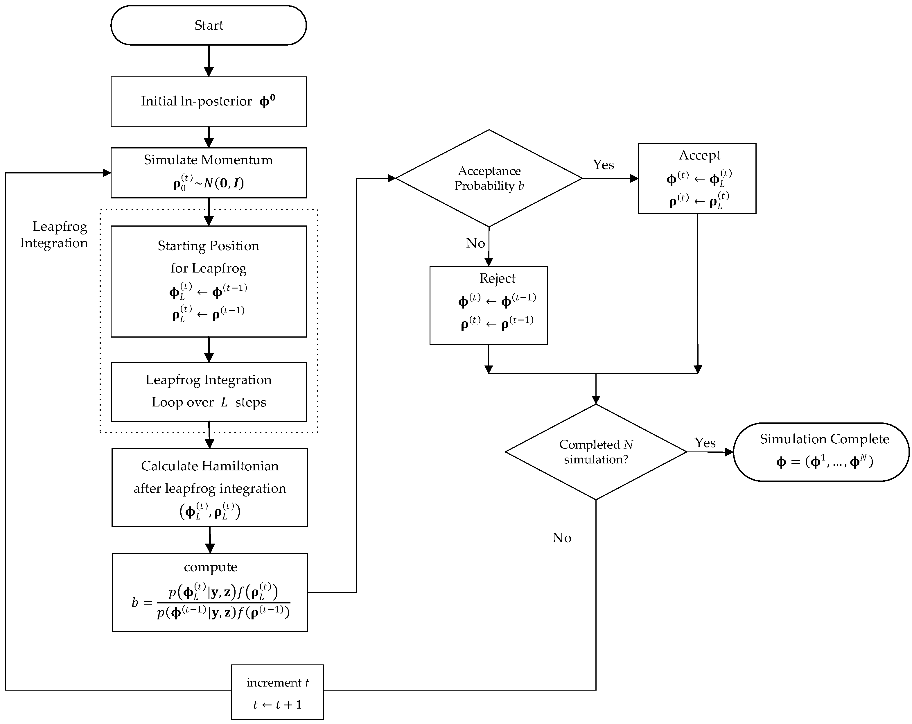
Perform the parameter estimation of Hibermimo using the HMC algorithm;

Algorithm 1 contains a pseudo-code for an implementation of the Hamiltonian algorithm for Hibermimo.

Algorithm 1 The Hamiltonian Monte Carlo for Hibermimo.

Step 6.

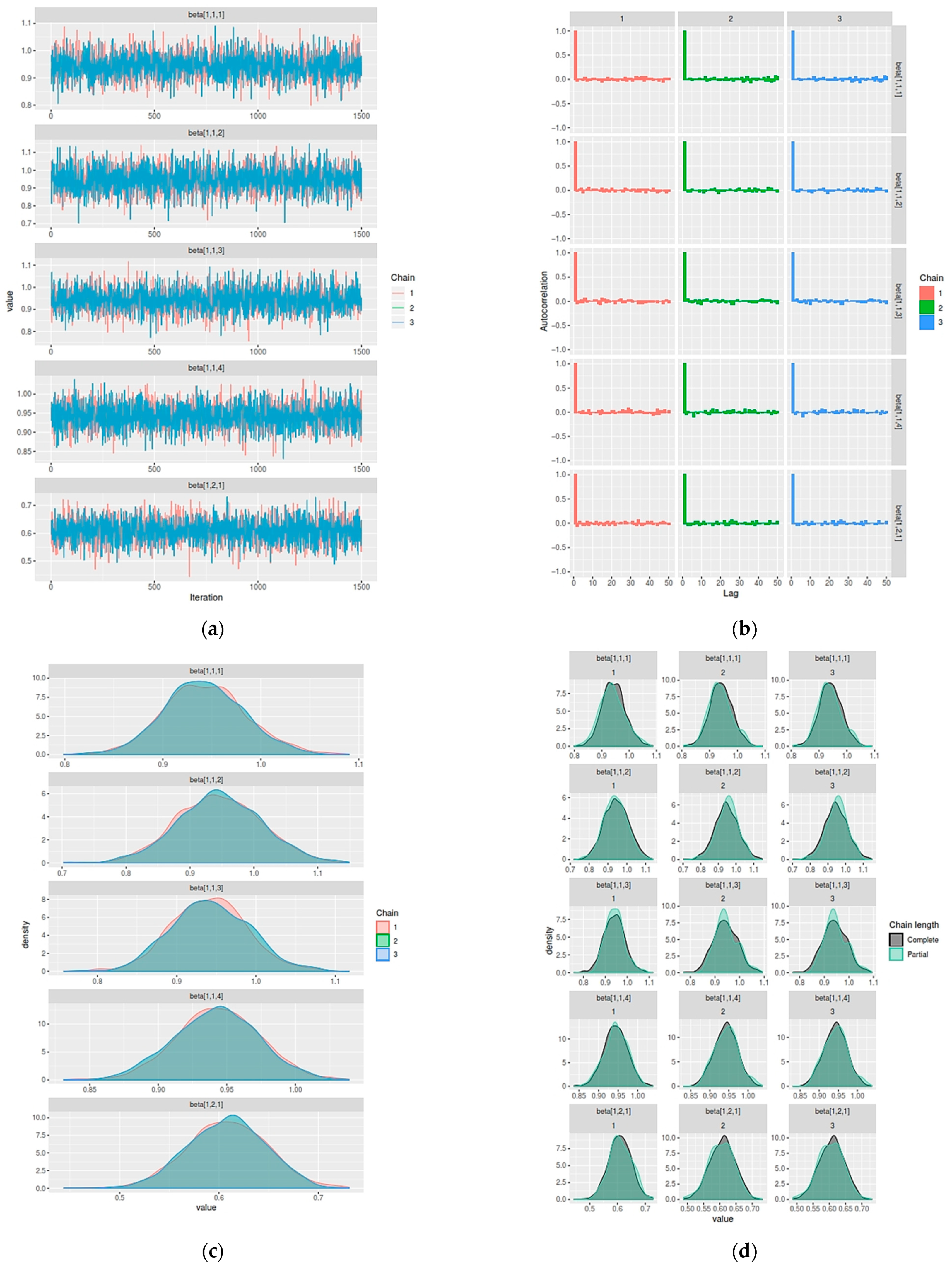
Monitor and evaluate the convergence of the algorithm.

Step 7.

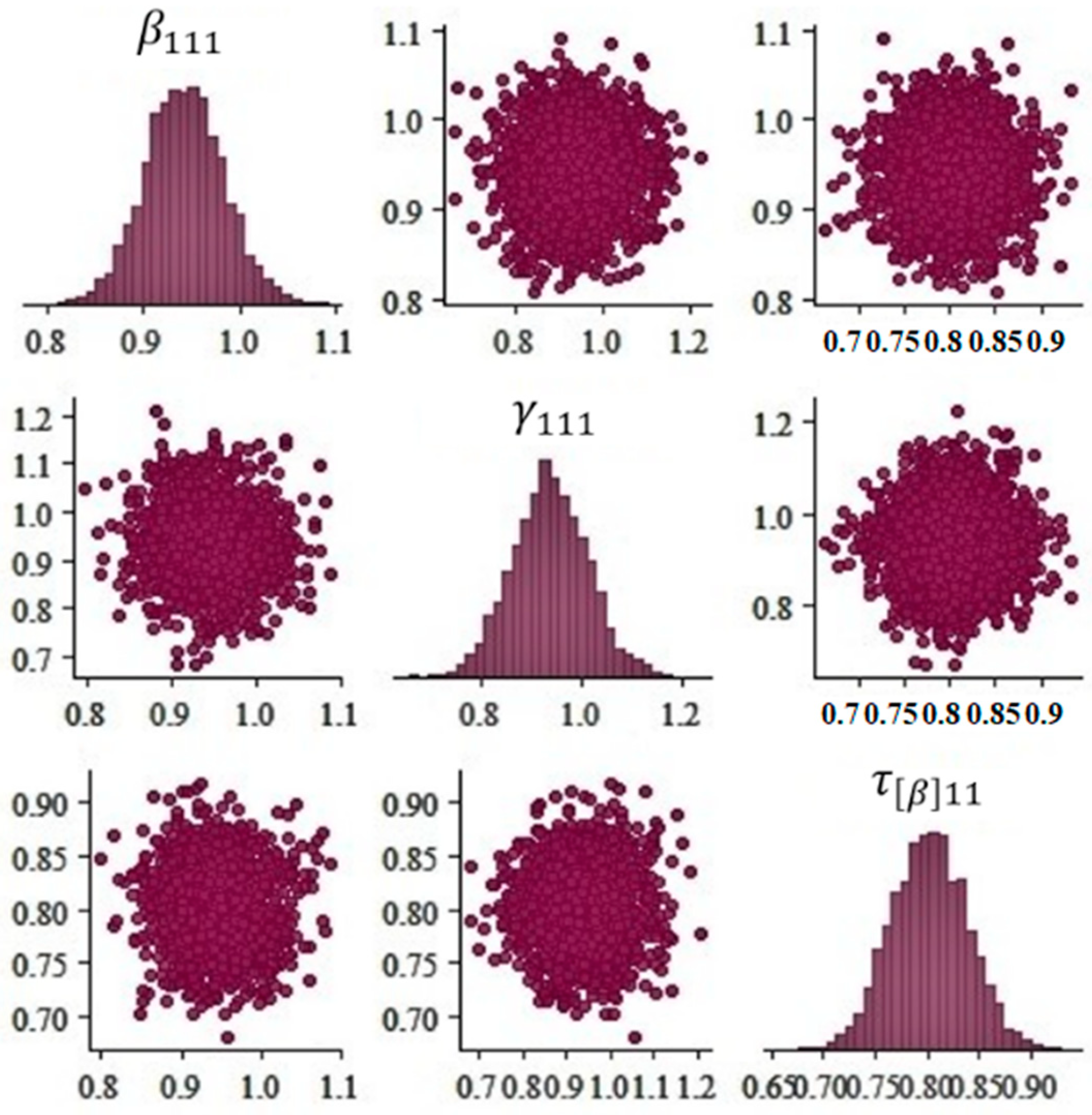
Plot the posterior distribution of Hibermimo.

Step 8.

Obtain a summary of the posterior distribution of Hibermimo.

HMC adopts a concept from physics to contain the local random walk performance in the Metropolis algorithm, which allows it to move much more quickly through the target distribution. HMC, which combines MCMC with a deterministic simulation method, is also called hybrid Monte Carlo. A multivariate normal distribution, $\mathsf{\rho }$, which is a ‘momentum’ variable, is added by HMC for each component $\mathsf{\varphi }$. Both $\mathsf{\varphi }$ and $\mathsf{\rho }$ are then updated together in a new Metropolis algorithm, in which the jumping distribution for $\mathsf{\varphi }$ is determined mainly by $\mathsf{\rho }$. Set the diagonal mass matrix $\mathit{I}$, the leapfrog integration step size $\in$ (indicating the leapfrog step jumps), the number of leapfrog integration steps $L$, and the number of iterations t. HMC has several steps of the iteration process described through the flowchart in Figure 2.

3. Results

3.1. Parameter Estimation of Hibermimo

The most challenging part of undertaking a Bayesian analysis is estimating the Bayesian model. The main difficulty is to analyze the statistical models with an appropriate algorithm and determine the prior knowledge for a specific model under consideration. Each parameter of the hierarchical model’s estimated value can be assigned after all the relevant priors have been given [28].

Parameter estimation for Hibermimo is calculated using the Bayesian HMC algorithm approach. Bayesian statistical analysis, in general, uses MCMC for fitting a wide range of complex models. MCMC produces a summary and diagnostic statistics by storing MCMC samples from the corresponding posterior distributions in output datasets for convergence analysis [29].

An alternative MCMC method, HMC [30,31,32], has grown increasingly popular because the algorithm’s novel properties can yield much better performance for general hierarchical models. Hibermimo, a complex Bayesian model, requires an HMC algorithm that corresponds to an MCMC technique. This algorithm combines the Metropolis Monte Carlo approach [33,34] and the Hamiltonian dynamics [35,36]. One of the MCMC algorithms applies the adaptive sampling extension No-U-Turn Sampler (NUTS) in some estimation programs. This research used Stan, a general-purpose software platform for fitting arbitrarily complex Bayesian models of the Hibermimo type that allows full inference using the HMC/NUTS strategy. Recently, both algorithms were included in Stan [37], making it an essential program with high-performance statistical computation for specifying a Bayesian model by counting the log of a probability density function.

3.2. Application

This section discusses the performance of Hibermimo applied to the Bidikmisi scholarship empirical case, which is a prototype of the district of East Java Province in 2015. We used social science data, with unique binary responses (0 and 1) identified as having a Bernoulli mixture distribution with a finite number of mixture components. This dataset was collected from the Ministry of Research and Technology and Higher Education database through the Bidikmisi Division. We set the Bidikmisi scholarship recipients as the micro-level data. Moreover, data on the social welfare indicators and statistics on people’s welfare for the East Java Province in 2015 were used for the macro-level data.

Explanations of the pre-processing identification technique used to construct the Bernoulli mixture distribution at the micro-level, the response variable $\left(Y\right),$ and the predictor variable at the micro-level $\left(X\right)$ were provided by Iriawan [2]. However, we changed the data scale for the predictor variable $X_{12}$ (fourth-semester ranking) and $X_{13}$ (fifth-semester ranking) into a ratio scale. The list of district characteristics, which were used as predictors at the macro-level $\left(W\right),$ is presented in

Table 1. Predictor variables at the macro-level.

Variable	Description	Data Scale
$W_1$	Percentage of the poverty population	Ratio
$W_2$	The average extent of school	Ratio
$W_3$	Percentage of population aged 19–24 out of school	Ratio
$W_4$	Percentage of households with roofs made from asbestos/zinc + bamboo/wood + straw/fiber/leaves/other	Ratio
$W_5$	Percentage of households with wooden walls	Ratio
$W_6$	Percentage of households receiving subsidies	Ratio
$W_7$	Percentage of households receiving insufficient student aid for high school students	Ratio
$W_8$	Percentage of households whose members have accessed the internet in the last 3 months	Ratio

.

Modeling of the Bidikmisi scholarship grantees with the district characteristics data was performed computationally by including the DAG Hibermimo structure into the program code. The modeling was carried out by using the Bayesian Bernoulli mixture aggregate regression model (BBMARM) and Hibermimo. Both models were analyzed using Stan and applying the HMC/NUTS algorithm. The significance of the model parameters was tested by using a credible interval, and the formation of a confidence interval was calculated by the highest posterior density (HPD) approach [22,24,38,39]. The estimated BBMARM was directly compared with the performance of Hibermimo.

3.2.1. Bayesian Bernoulli Mixture Aggregate Regression Model

The Bayesian Bernoulli Mixture aggregate regression model (BBMARM) was estimated by using the micro-level predictors coupled with the macro-level predictor variables together as one level. In this research, the analysis of the BBMARM design with the predictor variables involved both categorical and continuous variables, 22 dummy, and 12 continuous variables. Dummy variables were used in BBMARM to capture the influence of the categorical variables. The estimated parameters of this model produced as many as 35 parameters for each mixture component. We fitted BBMARM by using Stan with three chains running for 3000 iterations each. Stan automatically used half of the iterations as a warm-up and the other half for sampling [37]. The estimation results of Stan programming for BBMARM showed compatibility with the MCMC properties, i.e., they were irreducible, aperiodic, and recurrent. The monitoring convergence visually presented in the diagnostic plot includes historical plots, autocorrelation plots, and density plots [40]. The estimated parameters of BBMARM are provided in

Table 2. Estimation parameters of BBMARM.

Parameters	Mean	2.5%	50%	97.5%	n_eff	Rhat
${\pi }_1$	0.704	0.698	0.711	0.724	8717	1
${\pi }_2$	0.296	0.276	0.295	0.315	8717	1
${\beta }_{01}$	0.983	0.976	0.983	0.990	9511	1
${\beta }_{02}$	0.995	0.988	0.995	0.998	10,123	1
${\beta }_{11}$	0.040	0.028	0.040	0.051	2970	1
${\beta }_{12}$	0.025	0.015	0.025	0.034	4253	1
${\beta }_{21}$	0.025	0.015	0.025	0.035	3983	1
${\beta }_{22}$	−0.026	−0.035	−0.026	−0.016	3649	1
…	…	…	…	…	…	…
${\beta }_{331}$	0.176	0.162	0.176	0.190	2755	1
${\beta }_{332}$	0.018	0.005	0.018	0.030	2404	1
${\beta }_{341}$	0.095	0.082	0.095	0.108	3246	1
${\beta }_{342}$	−0.016	−0.042	−0.016	0.011	3896	1

Samples were drawn using NUTS. For each parameter, n_eff is a crude measure of the effective sample size, and Rhat is the potential scale reduction factor on split chains (at convergence, Rhat = 1).

.

Table 2 presents a summary of the parameter estimation results of BBMARM. The values of the nodes ${\beta }_{01}$ and ${\beta }_{02}$ denote the intercept of the mixture components 1 and 2, respectively. The significance of the BBMARM regression model parameters was tested using a credible interval. The estimated parameter is supposed to be not significant when zero lies inside the credible interval.

Based on Table 2, the characteristics of Bidikmisi acceptance that had a significant effect on the mixture of Components 1 and 2 are the mother’s occupation $\left(X_2\right)$, ownership of family homes $\left(X_5\right)$, the land area of family homes $\left(X_6\right)$, the extent of family residential buildings $\left(X_7\right)$, ownership of toilet and washing facilities $\left(X_8\right)$, the number of families in the household $\left(X_{10}\right)$, city distance $\left(X_{11}\right)$, and fourth-semester ranking $\left(X_{12}\right)$. The district characteristics that significantly influenced each mixture component were the percentage of households receiving subsidies $\left(W_6\right)$ and the percentage of households whose members had accessed the internet in the last 3 months $\left(W_8\right)$. The BBMARM for two mixture components can be formulated as follows:

$$\begin{array}{cc}\hfill \widehat{p}\left(\mathbf{y}|\mathsf{\omega }\right)& ={\displaystyle \sum _{c=1}^C}{\pi }_c{p}_c\left(y_i|{\theta }_{ic}\right)\hfill \\ & ={\pi }_1{p}_1\left(y_i|{\theta }_{i1}\right)+{\pi }_2{p}_2\left(y_i|{\theta }_{i2}\right)\hfill \\ & =0.704p_1\left(y_i|{\theta }_{i1}\right)+0.296p_2\left(y_i|{\theta }_{i2}\right).\hfill \end{array}$$

(17)

where ${\theta }_{ic}$ is an appropriate set of parameters with a Bernoulli distribution [41]. For the binary response, based on Kay and Little [42], we used the linearity property of the predictor “log” link function to connect the mean of ${\theta }_{ic}$ in concert with the micro-level predictor variables. The BBMARM for the probability mass function $p_c\left(y_i|{\theta }_{ic}\right)$ can be written as:

$$\begin{array}{l}{p}_c\left(y_i|{\theta }_{ic}\right)={\theta }_{ic}{}^{y_i}{\left(1-{\theta }_{ic}\right)}^{1-y_i}\\ \mathrm{for}c=1\\ \log \left[\frac{{\theta }_{i1}}{1-{\theta }_{i1}}\right]=0.983+0.040d_{111}+0.025d_{121}+0.058d_{131}-\cdots +0.095W_{81}\\ \mathrm{and}c=2\\ \log \left[\frac{{\theta }_{i2}}{1-{\theta }_{i2}}\right]=0.995+0.025d_{112}-0.026d_{122}-0.004d_{142}-\cdots -0.016W_{82}\end{array}$$

(18)

3.2.2. Hierarchical Bernoulli Mixture Model

The development of a hierarchical model for binary responses was first shown by Mason et al. [43], Goldstein [44], and Longford [45]. An earlier methodological framework for fitting a multilevel logit model was developed by Mason et al. [43], which obtained the maximum likelihood using the Bayes EM algorithm (REML/Bayes EM). Interest in these methodological and substantive algorithms directly encouraged Bryk and Raudenbush [46] and Goldstein [15,44] to extend multilevel models for linear data. Furthermore, Goldstein [44] implemented a generalized least square algorithm using educational data to measure the explanatory variables within a hierarchical structure. In supplementary improvement approximations, Goldstein and Rasbash [47] used the available software packages VARCL and ML3 to analyze multilevel models with binary responses, which Rodriguez and Goldman [48] had simulated to highlight the work. Besides, a Fisher scoring algorithm for fitting the general hierarchical model was developed by Longford [45]. Recently, we presented the Hibermimo, appropriating a Bayesian approach with Stan computation to apply the HMC algorithm.

Hibermimo has been applied for modeling Bidikmisi grantees, an East Java prototype, with four districts identified for scholarship applicants. The parameters at the micro-level include 22 dummy and four continuous variables. Moreover, the macro-level has eight continuous variables. Implementation of the Hibermimo conceptual estimation process was performed by the DAG shown in Figure 1. As it is a complex Bayesian model, Hibermimo requires an HMC algorithm that is compatible with the Markov Chain Monte Carlo (MCMC) technique, which combines the Metropolis Monte Carlo approach and the Hamiltonian dynamics’ advantages. The estimation parameters of the Hibermimo depend on the effectiveness of Stan software, an essential program with high-performance computational statistics for determining Bayesian models that compute the log of probability density functions. For the Hibermimo estimation process enabling full Bayesian inference, Stan used the HMC/NUTS procedure, running three chains with 3000 iterations each.

The estimation result is based on the output of the software Stan, the Hibermimo running process, obtained to meet the MCMC property’s suitability. Taylor and Karlin [49], including Boldstad [50], indicate that the convergence meeting strongly ergodic properties containing irreducible, aperiodic, and recurrent. The MCMC running process is done by running the iteration process parameter estimation. During the iteration, Stan will generate a diagnostic plot to monitor the MCMC process’s output that has reached an equilibrium condition. The indication of achieving this equilibrium condition can be seen in the graphics diagnostic plot’s grammar [51] and analyzed CODA diagnostic [52,53,54,55]. A visualization is a pivotal tool for Bayesian data analysis that can be used for setting up an initial prior value, ensuring the algorithm’s credibility, monitoring, and evaluating convergence of the algorithm to obtain Bayesian inference. Further, the visual of the graphics diagnostic plot is shown in Figure 3.

As shown in Figure 3, Stan can be enhanced by ggmcmc with the ggplot2 package with the aim of including the design and implementation of MCMC diagnostics, allowing Bayesian inference users to have better and more flexible visual diagnostic tools [56]. The diagnostic plot shows the monitoring of the estimation process of Hibermimo’s three chains of 3000 iterations each. The chains are displayed in different colors: red (Chain 1), green (Chain 2), and blue (Chain 3).

The serial plot of 3000 iterations, half as a warm-up and a half for sampling, generated Hibermimo estimates. The process of the sample products in the MCMC process showed no extreme values. As seen in Figure 3a, the serial plot shows random values with a pattern that tends to be stationary and random. Moreover, the aperiodic properties can be displayed by the serial plot pattern of the characteristics. Recurrence is illustrated by a serial plot showing stable parameter samples in a particular value domain. The autocorrelation plot in Figure 3b strengthens the evidence that the resulting sample of Hibermimo parameter estimates are random, indicated by the lag value, with only Lag 0 being close to zero at the subsequent lag. The density plot in Figure 3, which is visually symmetrical in shape for each chain, shows that the density estimation results for Hibermimo with three chains of 1500 iterations have a normal distribution. Based on the MCMC diagnostic plot, it can be concluded that the parameter estimation process has reached convergence. A convergence analysis with CODA diagnostic parameter estimation of Hibermimo with three chains and 1500 iterations found that a stationary test for all mixture parameters were “passed” as specifically convergent, based on Gelman–Rubin [52] diagnostics. Meanwhile, for Raftery–Lewis diagnostics in CODA [53], all parameters had a dependency factor (DF) of <5 in each chain, indicating a convergent condition. Moreover, by using the visual structure graphic diagnostics of Hibermimo, we obtained the “mcmc_pairs” function, which can also look at multiple parameters, including ${\beta }_{kjc}$, ${\gamma }_{qkc}$, and ${\tau }_{\left[\beta \right]kc}$. A square plot matrix with univariate marginal distributions along the diagonal as histograms and bivariate distributions of the diagonal as scatterplots is shown in Figure 4.

The univariate histograms and bivariate scatterplots for selected parameters in Figure 4 were used for identifying collinearity. As can be seen, the dots on the larger bivariate plot indicate that there are no correlating variables between the micro- and macro-levels. Furthermore, we can fit the Hibermimo because there is no indication of multicollinearity in each hierarchical level.

The Hibermimo parameter significance test, a two-level hierarchical model, uses a credible interval based on the Koop hypothesis [39]. If the credible interval contains a zero value, it concludes that the hypothesis can be rejected, which means that the estimated parameters are not significant.

Table 3. Estimation parameters of the Hibermimo micro-level model.

Parameter	Districts of Micro-Level Mix-1				Districts of Micro-Level Mix-2
	Bangkalan	Sampang	Pamekasan	Sumenep	Bangkalan	Sampang	Pamekasan	Sumenep
${\beta }_0$	0.943 (0.042)	0.944 (0.065)	0.942 (0.048)	0.943 (0.030)	0.607 (0.040)	0.610 (0.046)	0.608 (0.093)	0.608 (0.087)
${\beta }_1$	0.358 (0.012)	0.358 (0.019)	0.359 (0.036)	0.359 (0.012)	0.129 (0.076)	0.129 (0.033)	0.128 (0.072)	0.129 (0.040)
${\beta }_2$	0.052 (0.031)	0.051 (0.030)	0.051 (0.037)	0.051 (0.013)	0.284 (0.024)	0.286 (0.018)	0.285 (0.035)	0.285 (0.077)
${\beta }_3$	0.144 (0.047)	0.145 (0.018)	0.146 (0.010)	0.145 (0.017)	0.364 (0.052)	0.363 (0.019)	0.367 (0.018)	0.366 (0.083)
${\beta }_4$	0.283 (0.059)	0.284 (0.038)	0.284 (0.011)	0.283 (0.074)	0.425 (0.018)	0.429 (0.025)	0.428 (0.024)	0.427 (0.017)
${\beta }_5$	0.243 (0.090)	0.246 (0.020)	0.243 (0.019)	0.243 (0.037)	0.390 (0.013)	0.391 (0.085)	0.390 (0.017)	0.391 (0.013)
${\beta }_6$	0.444 (0.029)	0.447 (0.046)	0.447 (0.048)	0.446 (0.046)	0.355 (0.027)	0.357 (0.051)	0.355 (0.018)	0.355 (0.074)
${\beta }_7$	0.161 (0.068)	0.162 (0.033)	0.162 (0.010)	0.161 (0.014)	0.331 (0.020)	0.332 (0.014)	0.331 (0.014)	0.331 (0.014)
${\beta }_8$	0.208 (0.035)	0.209 (0.014)	0.209 (0.093)	0.208 (0.011)	0.286 (0.063)	0.287 (0.013)	0.285 (0.016)	0.286 (0.013)
${\beta }_9$	0.241 (0.093)	0.242 (0.035)	0.242 (0.021)	0.242 (0.013)	0.037 (0.023)	0.038 (0.006)	0.037 (0.028)	0.037 (0.010)
${\beta }_{10}$	0.424 (0.010)	0.427 (0.034)	0.424 (0.087)	0.424 (0.015)	0.082 (0.001)	0.083 (0.001)	0.080 (0.002)	0.082 (0.004)
${\beta }_{11}$	0.104 (0.077)	0.106 (0.014)	0.103 (0.075)	0.103 (0.094)	0.116 (0.059)	0.117 (0.067)	0.115 (0.078)	0.116 (0.028)
${\beta }_{12}$	0.084 (0.007)	0.086 (0.005)	0.086 (0.008)	0.085 (0.005)	0.391 (0.012)	0.393 (0.015)	0.390 (0.026)	0.390 (0.014)
${\beta }_{13}$	0.092 (0.004)	0.095 (0.004)	0.090 (0.002)	0.092 (0.002)	0.490 (0.021)	0.494 (0.031)	0.493 (0.020)	0.492 (0.015)
${\beta }_{14}$	0.352 (0.010)	0.354 (0.017)	0.351 (0.030)	0.352 (0.017)	0.256 (0.013)	0.256 (0.019)	0.255 (0.007)	0.255 (0.022)
${\beta }_{15}$	0.181 (0.001)	0.183 (0.008)	0.181 (0.007)	0.181 (0.009)	0.320 (0.009)	0.323 (0.007)	0.322 (0.016)	0.321 (0.091)
${\beta }_{16}$	0.583 (0.017)	0.587 (0.013)	0.584 (0.028)	0.584 (0.020)	0.108 (0.071)	0.108 (0.090)	0.110 (0.023)	0.109 (0.086)
${\beta }_{17}$	0.231 (0.011)	0.233 (0.010)	0.232 (0.063)	0.232 (0.089)	0.415 (0.065)	0.420 (0.016)	0.407 (0.013)	0.411 (0.011)
${\beta }_{18}$	0.083 (0.001)	0.084 (0.002)	0.084 (0.004)	0.083 (0.003)	0.169 (0.043)	0.166 (0.013)	0.170 (0.039)	0.169 (0.011)
${\beta }_{19}$	0.185 (0.013)	0.187 (0.015)	0.187 (0.020)	0.186 (0.016)	0.121 (0.069)	0.123 (0.013)	0.122 (0.066)	0.122 (0.068)
${\beta }_{20}$	0.083 (0.004)	0.068 (0.004)	0.059 (0.004)	0.071 (0.002)	0.141 (0.046)	0.140 (0.029)	0.144 (0.067)	0.143 (0.046)
${\beta }_{21}$	0.412 (0.019)	0.414 (0.020)	0.414 (0.013)	0.413 (0.014)	0.214 (0.014)	0.218 (0.024)	0.211 (0.032)	0.212 (0.071)
${\beta }_{22}$	0.621 (0.058)	0.163 (0.029)	0.621 (0.053)	0.162 (0.060)	0.096 (0.010)	0.096 (0.003)	0.099 (0.013)	0.097 (0.069)
${\beta }_{23}$	−0.398 (0.042)	−0.401 (0.013)	−0.398 (0.008)	−0.398 (0.012)	0.285 (0.052)	0.286 (0.011)	0.285 (0.015)	0.285 (0.016)
${\beta }_{24}$	0.526 (0.009)	0.252 (0.017)	0.540 (0.016)	0.254 (0.097)	0.564 (0.072)	0.568 (0.098)	0.567 (0.085)	0.566 (0.090)
${\beta }_{25}$	0.262 * (0.011)	0.267 * (0.046)	0.265 * (0.011)	0.266 * (0.077)	0.326 * (0.010)	0.328 * (0.047)	0.328 * (0.023)	0.327 * (0.018)
${\beta }_{26}$	0.596 * (0.065)	0.581 * (0.034)	0.606 * (0.019)	0.599 * (0.029)	0.881 * (0.064)	0.885 * (0.012)	0.879 * (0.016)	0.881 * (0.019)

Note: * the parameter estimate is not significant at α = 5%.

shows that the estimation results of Hibermimo for the micro-level parameters in component Mixture 1 and Mixture 2 that are not significant in all districts are the variables $X_{12}$ (fourth-semester ranking) and $X_{13}$ (fifth-semester ranking). The parentheses below the estimated mean values denote the standard deviation of each beta parameter. Moreover, all the characteristics of the students applying for the Bidikmisi scholarship were significant in the four districts. This means that the characteristics of the Bidikmisi registration form had a significant effect on the acceptance of Bidikmisi scholarships in each district. Based on Table 3, the Hibermimo model for two mixture components can be formulated as follows:

$$\begin{array}{cc}\hfill \widehat{p}\left(\mathbf{y}|\mathsf{\omega }\right)& ={\displaystyle \sum _{c=1}^C}{\pi }_c{p}_c\left(y_{ij}|{\theta }_{ijc}\right)\hfill \\ & ={\pi }_1{p}_1\left(y_{ij}|{\theta }_{ij1}\right)+{\pi }_2{p}_2\left(y_{ij}|{\theta }_{ij2}\right)\hfill \\ & =0.714p_1\left(y_{ij}|{\theta }_{ij1}\right)+0.286p_2\left(y_{ij}|{\theta }_{ij2}\right).\hfill \end{array}$$

(19)

Hibermimo’s posterior summary of the estimation of the micro-level parameters, including the mean and standard deviation (in parentheses), are reported in Table 3.

The Hibermimo micro-level model for $j=1$, Bangkalan City, can be written as follows:

$$\begin{array}{l}{p}_c\left(y_{ij}|{\theta }_{ijc}\right)={\theta }_{ijc}{}^{y_{ij}}{\left(1-{\theta }_{ijc}\right)}^{1-y_{ij}}\\ \mathrm{for}c=1\mathrm{and}j=1\\ \log \left[\frac{{\theta }_{i11}}{1-{\theta }_{i11}}\right]=0.943+0.358d_{11\left(i11\right)}+0.052d_{12\left(i11\right)}+\cdots +0.596X_{13\left(i11\right)}\\ \\ \mathrm{and}c=2\mathrm{and}j=1\\ \log \left[\frac{{\theta }_{i12}}{1-{\theta }_{i12}}\right]=0.607+0.129d_{11\left(i12\right)}+0.284d_{12\left(i12\right)}+\cdots +0.881X_{13\left(i12\right)}.\end{array}$$

(20)

A summary of estimation results of the Hierarchical Bernoulli mixture model (Hibermimo) for the macro-level Mixture 1 components is presented in

Table 4. Estimation parameter of the Hibermimo macro-level model for Mixture 1 component.

${\mathit{\beta }}_{\mathit{k}\mathit{j}\mathit{c}}$	Macro-Level Parameters (${\mathit{\gamma }}_{\mathit{q}\mathit{k}\mathit{c}}$)
	${\mathit{\gamma }}_{\mathbf{0}\mathit{k}\mathbf{1}}$	${\mathit{\gamma }}_{\mathbf{1}\mathit{k}\mathbf{1}}$	${\mathit{\gamma }}_{\mathbf{2}\mathit{k}\mathbf{1}}$	${\mathit{\gamma }}_{\mathbf{3}\mathit{k}\mathbf{1}}$	${\mathit{\gamma }}_{\mathbf{4}\mathit{k}\mathbf{1}}$	${\mathit{\gamma }}_{\mathbf{5}\mathit{k}\mathbf{1}}$	${\mathit{\gamma }}_{\mathbf{6}\mathit{k}\mathbf{1}}$	${\mathit{\gamma }}_{\mathbf{7}\mathit{k}\mathbf{1}}$	${\mathit{\gamma }}_{\mathbf{8}\mathit{k}\mathbf{1}}$
${\beta }_{0j1}$	0.936 (0.076)	0.002 (0.008)	0.003 (0.003)	0.008 (0.001)	0.001 (0.003)	0.001 (0.002)	0.002 (0.002)	0.010 (0.002)	0.005 (0.004)
${\beta }_{1j1}$	0.356 (0.011)	0.002 (0.006)	0.001 (0.007)	0.002 (0.005)	0.007 (0.005)	0.001 (0.007)	0.002 (0.009)	0.004 (0.002)	0.007 (0.002)
${\beta }_{2j1}$	0.053 (0.004)	0.003 (0.008)	0.001 (0.003)	0.002 (0.001)	0.003 (0.001)	0.0001 (0.001)	0.001 (0.002)	0.008 (0.001)	0.002 (0.001)
${\beta }_{3j1}$	0.142 (0.020)	0.001 (0.001)	0.007 (0.010)	0.001 (0.002)	0.002 (0.001)	0.001 (0.002)	0.006 (0.001)	0.001 (0.001)	0.009 (0.012)
${\beta }_{4j1}$	0.278 (0.030)	0.002 (0.003)	0.009 (0.002)	0.003 (0.005)	0.003 (0.004)	0.002 (0.003)	0.006 (0.009)	0.003 (0.004)	0.007 (0.002)
${\beta }_{5j1}$	0.239 (0.027)	0.001 (0.001)	0.003 (0.003)	0.002 (0.002)	0.001 (0.002)	0.009 (0.001)	0.005 (0.007)	0.004 (0.004)	0.006 (0.007)
${\beta }_{6j1}$	0.444 (0.032)	0.004 (0.005)	0.010 (0.018)	0.004 (0.004)	0.015 (0.011)	0.002 (0.006)	0.010 (0.013)	0.010 (0.009)	0.020 (0.023)
${\beta }_{7j1}$	0.159 (0.014)	0.001 (0.003)	0.007 (0.001)	0.001 (0.001)	0.005 (0.003)	0.002 (0.002)	0.003 (0.003)	0.002 (0.001)	0.002 (0.005)
${\beta }_{8j1}$	0.203 (0.062)	0.004 (0.003)	0.004 (0.008)	0.002 (0.001)	0.001 (0.001)	0.002 (0.001)	0.006 (0.003)	0.002 (0.001)	0.001 (0.002)
${\beta }_{9j1}$	0.239 (0.036)	0.003 (0.004)	0.002 (0.002)	0.002 (0.002)	0.005 (0.006)	0.002 (0.002)	0.005 (0.005)	0.004 (0.001)	0.002 (0.002)
${\beta }_{10j1}$	0.414 (0.087)	0.018 (0.002)	0.011 (0.002)	0.003 (0.003)	0.007 (0.001)	0.007 (0.007)	0.009 (0.003)	0.003 (0.003)	0.008 (0.010)
${\beta }_{11j1}$	0.100 (0.015)	0.007 (0.001)	0.004 (0.001)	0.001 (0.002)	0.002 (0.003)	0.008 (0.0004)	0.003 (0.004)	0.001 (0.001)	0.004 (0.005)
${\beta }_{12j1}$	0.092 (0.013)	0.002 (0.001)	0.003 (0.005)	0.010 (0.001)	0.005 (0.001)	0.007 (0.001)	0.004 (0.006)	0.002 (0.001)	0.008 (0.012)
${\beta }_{13j1}$	0.080 (0.009)	0.051 (0.007)	0.005 (0.001)	0.0002 (0.001)	0.001 (0.002)	0.002 (0.002)	0.002 (0.002)	0.008 (0.001)	0.008 (0.001)
${\beta }_{14j1}$	0.338 (0.026)	0.006 (0.007)	0.005 (0.009)	0.012 (0.015)	0.011 (0.017)	0.005 (0.009)	0.005 (0.004)	0.004 (0.003)	0.002 (0.011)
${\beta }_{15j1}$	0.177 (0.021)	0.002 (0.003)	0.004 (0.004)	0.002 (0.003)	0.005 (0.006)	0.007 (0.004)	0.003 (0.005)	0.002 (0.001)	0.009 (0.013)
${\beta }_{16j1}$	0.577 (0.015)	0.004 (0.002)	0.005 (0.004)	0.004 (0.003)	0.010 (0.006)	0.007 (0.004)	0.006 (0.006)	0.011 (0.010)	0.020 (0.016)
${\beta }_{17j1}$	0.226 (0.013)	0.002 (0.005)	0.008 (0.012)	0.004 (0.002)	0.002 (0.003)	0.002 (0.005)	0.007 (0.005)	0.004 (0.004)	0.003 (0.007)
${\beta }_{18j1}$	0.080 (0.006)	0.001 (0.001)	0.006 (0.001)	0.001 (0.001)	0.003 (0.003)	0.002 (0.001)	0.002 (0.002)	0.009 (0.002)	0.001 (0.002)
${\beta }_{19j1}$	0.181 (0.023)	0.002 (0.003)	0.006 (0.005)	0.002 (0.002)	0.008 (0.009)	0.002 (0.004)	0.009 (0.011)	0.003 (0.004)	0.011 (0.013)
${\beta }_{20j1}$	0.092 (0.008)	0.006 (0.001)	0.001 (0.002)	0.002 (0.001)	0.002 (0.002)	0.005 (0.001)	0.088 (0.002)	0.009 (0.001)	0.003 (0.004)
${\beta }_{21j1}$	0.409 (0.029)	0.004 (0.003)	0.012 (0.011)	0.001 (0.002)	0.005 (0.010)	0.002 (0.002)	0.012 (0.010)	0.003 (0.007)	0.004 (0.004)
${\beta }_{22j1}$	0.158 (0.072)	0.003 (0.004)	0.003 (0.002)	0.003 (0.001)	0.002 (0.002)	0.002 (0.002)	0.002 (0.002)	0.002 (0.001)	0.008 (0.006)
${\beta }_{23j1}$	−0.390 (0.013)	−0.005 (0.004)	−0.004 (0.001)	−0.007 (0.0003)	−0.0004 (0.001)	−0.004 (0.0003)	−0.006 (0.001)	−0.001 (0.000)	−0.0003 (0.001)
${\beta }_{24j1}$	0.250 (0.035)	0.003 (0.004)	0.009 (0.003)	0.002 (0.003)	0.006 (0.008)	0.008 (0.002)	0.001 (0.002)	0.008 (0.002)	0.004 (0.007)
${\beta }_{25j1}$	0.254 (0.019)	0.008 (0.001)	0.010 (0.007)	0.004 (0.003)	0.005 (0.005)	0.003 (0.003)	0.003 (0.003)	0.040 (0.004)	0.011 (0.009)
${\beta }_{26j1}$	0.657 (0.024)	0.056 (0.011)	0.053 (0.016)	0.044 (0.009)	0.057 (0.006)	0.045 (0.031)	0.001 (0.049)	0.036 (0.017)	0.092 (0.032)

. The parentheses below the estimated mean value contain the standard deviation of each gamma parameter. Among the macro-level variables, all model parameters were statistically significant, meaning that socio-economic characteristics of the district influence the probability of students receiving Bidikmisi scholarships. This study assumes that the aspects of a district generally affect the binary response. It presumes that the features of the macro-level have a positive relationship with a response. Furthermore, the number of families in the household (per person) harms the status of the scholarship recipient for a Mixture 1 component. As mentioned, the individual variables included the following: father’s job $\left(X_1\right)$, mother’s job $\left(X_2\right)$, father’s education $\left(X_3\right)$, mother’s education $\left(X_4\right)$, ownership of family homes $\left(X_5\right)$, land area of family homes $\left(X_6\right)$, the extent of family residential buildings $\left(X_7\right)$, ownership of toilet washing facilities $\left(X_8\right)$, water source used by the family $\left(X_9\right)$, number of families in the household (per person) $\left(X_{10}\right)$, city distance $\left(X_{11}\right)$, fourth-semester ranking $\left(X_{12}\right)$, and fifth-semester ranking $\left(X_{13}\right)$.

Empirical studies that have examined the determinants of the uniqueness of a binary response identified as having a Bernoulli finite mixture distribution in terms of a single structure have dealt separately with Bayesian Bernoulli Mixture Aggregate Regression Model and a Hibermimo micro-level model. This study utilized a multilevel model because the socio-economic features of districts affected the recipients of Bidikmisi scholarship decisions. Since the dependent variable was binary, Hibermimo constructed two sub-models: the micro-level model dealt with individual variables, and the macro-level model dealt with district variables.

In the results of the Hibermimo macro-level model for Mixture 1 component, the proportions of Mixture 1 and Mixture 2 components, respectively, are 0.714 and 0.286. The Hibermimo of the macro-level model for $c=1$ with the coefficient of gamma for Mixture 1 component is specified as follows:

$$\begin{array}{l}{\beta }_{0j1}=0.936+0.002W_{1j1}+0.003W_{2j1}+0.008W_{3j1}+0.001W_{4j1}+\\ 0.001W_{5j1}+0.002W_{6j1}+0.010W_{7j1}+0.005W_{8j1},\\ {\beta }_{1j1}=0.356+0.002W_{1j1}+0.001W_{2j1}+0.002W_{3j1}+0.007W_{4j1}+\\ 0.001W_{5j1}+0.002W_{6j1}+0.004W_{7j1}+0.007W_{8j1},\\ \mathrm{and}\mathrm{for}k=26\\ {\beta }_{26j1}=0.657+0.056W_{1j1}+0.053W_{2j1}+0.044W_{3j1}+0.057W_{4j1}+\\ 0.045W_{5j1}+0.001W_{6j1}+0.036W_{7j1}+0.092W_{8j1}.\end{array}$$

(21)

4. Discussion

The uniqueness of the two mixture components in this study was formed using two alternative models. The first model used only one level of aggregate regression, specifically BBMARM, and the second model used a multilevel model, which is Hibermimo.

Table 5. Selection of the best model with WAIC.

Model	WAIC
Bayesian Bernoulli Mixture aggregate regression model (BBMARM)	2392.3
Hierarchical Bernoulli mixture model (Hibermimo)	1218.9

presents the Widely Applicable Information Criteria (WAIC) values used for measuring the quality of the best designs. The WAIC successfully demonstrated the prediction accuracy estimation of the Bayesian model using log-likelihood, which was evaluated in a posterior simulation of parameter values. It has several advantages over general estimates, such as akaike information criterion (AIC) and deviance information criterion (DIC), which are mainly used in mixture modeling [57]. The best model is selected by comparing the WAIC for each model; the results are presented in Table 5.

The WAIC value of the Hibermimo is smaller than that of the BBMARM. Hibermimo has thus demonstrated its ability to support modelling of binary response identified as having a Bernoulli distribution with two mixture components.

5. Conclusions

In this study, our motivation is to develop a unique data-driven model in its binary response. The data-driven approach that we developed through combining the concept of hierarchical structure with the Bernoulli Mixture Model (BMM) has been able to provide new findings. As a follow-up to our new model design, the Hierarchical Bernoulli mixture model (Hibermimo), both its architecture and computational methods, have been studied theoretically and empirically. The Hibermimo was compared with the Bayesian Bernoulli mixture aggregate regression model (BBMARM), both of which were analyzed using Stan software with the HMC/NUTS algorithm. Furthermore, to determine the model’s effectiveness, we compared Hibermimo with BBMARM using WAIC.

The Monte Carlo Hamiltonian algorithm with a No-U-Turn sampler (HMC/NUTS) attracted considerable interest for implementation in the proposed Hibermimo model. The micro-level of Hibermimo is considered the symmetric link (logit). The logit link function provides a relationship between the linear predictors and the Bernoulli mixture distribution’s average utility.

The study has performed a compatible syntax program computation utilizing the HMC/NUTS algorithm for analyzing the BBMARM model and Hibermimo. In the model estimation, Hibermimo yielded a result of ~90% compliance with the modeling of each district. A selection of the best model with the WAIC value showed that Hibermimo was more able to accommodate the unique data-driven distribution of the Bernoulli mixture. Hibermimo could capture the phenomenon of mixing between observations in social science dimensions, which focuses on tracing the relationship between the unit of observation and the social environment.

We only compare the performance of Hibermimo with BBMARM because both have a Bernoulli distribution with a finite mixture, analyzed using the same software and the same HMC/NUTS algorithm but with different steps. We have not compared the model with other analytical methods because we focus on the development of novelties that we find both in terms of the mixture architecture and its computational approaches. However, based on the uniqueness of the data-driven Bernoulli Mixture that we found, we compared the Bernoulli Mixture model with several methods based on the achievement of the accuracy value applied to the problem of distributing Bidikmisi scholarships in East Java. These methods include the BMM, random forest, and SMOTE-Bagging. Based on the Area Under Curve (AUC) and geometric mean (g-mean) values, the BMM using the Gibbs Sampler algorithm run in Software Open-Bugs performs better than the random forest and SMOTE-Bagging [2]. For further research, a comparison between Hibermimo with random forest and SMOTE-Bagging which accommodates the mixture architecture with equivalent computational methods and analyzed using appropriate assays is highly recommended.

Moreover, the application of Hibermimo to the social science dataset using the symmetrical logit link function demonstrated exemplary performance. Future research should consider a flexible link function from a new class of generalized logistic distribution, namely a flexible generalized logit (Glogit) link, based on the simulation research of Prasetyo et al. [58]. The Glogit link is likely a good option and could be used in practice due to its flexibility.

References

1. Duda, R.O.; Hart, P.E.; Stork, D.G. Pattern Classification, 2nd ed.; Wiley-Interscience: Hoboken, NJ, USA, 2000; ISBN 0-471-05669-3. [Google Scholar]
2. Iriawan, N.; Fithriasari, K.; Ulama, B.S.S.; Suryaningtyas, W.; Pangastuti, S.S.; Cahyani, N.; Qadrini, L. On The Comparison: Random Forest, SMOTE-Bagging, and Bernoulli Mixture to Classify Bidikmisi Dataset in East Java. In Proceedings of the 2018 International Conference on Computer Engineering, Network and Intelligent Multimedia (CENIM), Surabaya, Indonesia, 26–27 November 2018; pp. 137–141. [Google Scholar]
3. Grim, J.; Pudil, P.; Somol, P. Multivariate Structural Bernoulli Mixtures for Recognition of Handwritten Numerals. In Proceedings of the Proceedings 15th International Conference on Pattern Recognition. ICPR-2000, Barcelona, Spain, 3–7 September 2000; Volume 2, pp. 585–589. [Google Scholar]
4. González, J.; Juan, A.; Dupont, P.; Vidal, E.; Casacuberta, F. Pattern Recognition and Image Analysis. In Proceedings of the Pattern Recognition and Image Analysis, Universitat Jaume I, Servei de Comunicació i Publicacions, Benicasim, Spain, 16–18 May 2001. [Google Scholar]
5. Juan, A.; Vidal, E. On the Use of Bernoulli Mixture Models for Text Classification. Pattern Recognit. 2002, 35, 2705–2710. [Google Scholar] [CrossRef]
6. Juan, A.; Vidal, E. Bernoulli Mixture Models for Binary Images. In Proceedings of the 17th International Conference on Pattern Recognition, 2004, ICPR 2004, Cambridge, UK, 26 August 2004; Volume 3, pp. 367–370. [Google Scholar]
7. Patrikainen, A.; Mannila, H. Subspace Clustering of High-Dimensional Binary Data—A Probabilistic Approach. In Proceedings of the In Workshop on Clustering High Dimensional Data and its Applications, SIAM International Conference on Data Mining, Lake Buena Vista, FL, USA, 24 April 2004. [Google Scholar]
8. Bouguila, N. On Multivariate Binary Data Clustering and Feature Weighting. Comput. Stat. Data Anal. 2010, 54, 120–134. [Google Scholar] [CrossRef]
9. Zhu, S.; Takigawa, I.; Zhang, S.; Mamitsuka, H. A Probabilistic Model for Clustering Text Documents with Multiple Fields. In Advances in Information Retrieval; Lecture Notes in Computer Science; Springer: Berlin/Heidelberg, Germany, 2007; Volume 4425, pp. 331–342. ISBN 978-3-540-71494-1. [Google Scholar]
10. Sun, Z.; Rosen, O.; Sampson, A.R. Multivariate Bernoulli Mixture Models with Application to Postmortem Tissue Studies in Schizophrenia. Biometrics 2007, 63, 901–909. [Google Scholar] [CrossRef] [Green Version]
11. Tikka, J.; Hollmén, J.; Myllykangas, S. Mixture Modeling of DNA Copy Number Amplification Patterns in Cancer. In Computational and Ambient Intelligence; Sandoval, F., Prieto, A., Cabestany, J., Graña, M., Eds.; Lecture Notes in Computer Science; Springer: Berlin/Heidelberg, Germany, 2007; Volume 4507, pp. 972–979. ISBN 978-3-540-73006-4. [Google Scholar]
12. Myllykangas, S.; Tikka, J.; Böhling, T.; Knuutila, S.; Hollmén, J. Classification of Human Cancers Based on DNA Copy Number Amplification Modeling. BMC Med. Genom. 2008, 1, 15. [Google Scholar] [CrossRef] [Green Version]
13. Saeed, M.; Javed, K.; Atique Babri, H. Machine Learning Using Bernoulli Mixture Models: Clustering, Rule Extraction and Dimensionality Reduction. Neurocomputing 2013, 119, 366–374. [Google Scholar] [CrossRef]
14. Hox, J.J. Multilevel Analysis: Techniques and Applications, 2nd ed.; Quantitative Methodology Series; Routledge, Taylor & Francis: New York, NY, USA, 2010; ISBN 978-1-84872-845-5. [Google Scholar]
15. Goldstein, H. Multilevel Statistical Models, 4th ed.; Wiley Series in Probability and Statistics; Wiley: Chichester, UK, 2011; ISBN 978-0-470-74865-7. [Google Scholar]
16. Hox, J.J. Applied Multilevel Analysis; TT-Publikaties: Amsterdam, The Netherlands, 1995; ISBN 978-90-801073-2-8. [Google Scholar]
17. Ismartini, P.; Iriawan, N.; Setiawan; Ulama, B.S.S. Toward a Hierarchical Bayesian Framework for Modelling the Effect of Regional Diversity on Household Expenditure. J. Math. Stat. 2012, 8, 283–291. [Google Scholar] [CrossRef] [Green Version]
18. Ringdal, K. Recent Developments in: Methods for Multilevel Analysis. Acta Sociol. 1992, 35, 235–243. [Google Scholar] [CrossRef]
19. Suryaningtyas, W.; Iriawan, N.; Fithriasari, K.; Ulama, B.; Susanto, I.; Pravitasari, A. On The Bernoulli Mixture Model for Bidikmisi Scholarship Classification with Bayesian MCMC. J. Phys. Conf. Ser. 2018, 1090, 012072. [Google Scholar] [CrossRef]
20. Carpenter, B.; Gelman, A.; Hoffman, M.D.; Lee, D.; Goodrich, B.; Betancourt, M.; Brubaker, M.; Guo, J.; Li, P.; Riddell, A. Stan: A Probabilistic Programming Language. J. Stat. Soft. 2017, 76, 1–32. [Google Scholar] [CrossRef] [Green Version]
21. McLachlan, G.; Peel, D. Finite Mixture Models; John Wiley and Sons: New York, NY, USA, 2000; ISBN 0-471-00626-2. [Google Scholar]
22. King, R.; Morgan, B.J.T.; Gimenez, O.; Brooks, S.P. Bayesian Analysis for Population Ecology; Interdisciplinary Statistics Series; Chapman & Hall/CRC: Boca Raton, FL, USA, 2010; ISBN 978-1-4398-1187-0. [Google Scholar]
23. Carlin, B.P.; Chib, S. Bayesian Model Choice via Markov Chain Monte Carlo Methods. J. R. Stat. Soc. Ser. B 1995, 57, 473–484. [Google Scholar] [CrossRef]
24. Box, G.E.P.; Tiao, G.C. Bayesian Inference in Statistical Analysis; Addison-Wesley Series in Behavioral Science; Addison-Wesley: Reading, MA, USA, 1973; ISBN 978-0-201-00622-3. [Google Scholar]
25. Guo, G.; Zhao, H. Multilevel Modeling for Binary Data. Annu. Rev. Sociol. 2000, 26, 441–462. [Google Scholar] [CrossRef]
26. Gelman, A.; Carlin, J.B.; Stern, H.S.; Dunson, D.B.; Vehtari, A.; Rubin, D.B. Bayesian Data Analysis, 3rd ed.; CRC Press: Boca Raton, FL, USA, 2014; ISBN 978-1-4398-9820-8. [Google Scholar]
27. Solikhah, A.; Kuswanto, H.; Iriawan, N.; Fithriasari, K. Fisher’s z Distribution-Based Mixture Autoregressive Model. Econometrics 2021, 9, 27. [Google Scholar] [CrossRef]
28. Gamerman, D. Markov Chain Monte Carlo for Dynamic Generalised Linear Models. Biometrika 1998, 85, 215–227. [Google Scholar] [CrossRef]
29. Iriawan, N.; Fithriasari, K.; Ulama, B.S.S.; Susanto, I.; Suryaningtyas, W.; Pravitasari, A.A. On the Markov Chain Monte Carlo Convergence Diagnostic of Bayesian Bernoulli Mixture Regression Model for Bidikmisi Scholarship Classification. In Proceedings of the Third International Conference on Computing, Mathematics and Statistics (iCMS2017), Langkawi, Malaysia, 7–8 November 2017; Kor, L.-K., Ahmad, A.-R., Idrus, Z., Mansor, K.A., Eds.; Springer: Singapore, 2019; pp. 397–403, ISBN 978-981-13-7279-7. [Google Scholar]
30. Wang, Z.; Mohamed, S.; De Freitas, N. Adaptive Hamiltonian and Riemann Manifold Monte Carlo Samplers. In Proceedings of the 30th International Conference on Machine Learning, Proceedings of Machine Learning Research (PMLR), Atlanta, GA, USA, 17–19 June 2013; Volume 28, pp. 1462–1470. [Google Scholar]
31. Hoffman, M.D.; Gelman, A. The No-U-Turn Sampler: Adaptively Setting Path Lengths in Hamiltonian Monte Carlo. J. Mach. Learn. Res. 2014, 15, 1593–1623. [Google Scholar]
32. Grantham, N.S. Clustering Binary Data with Bernoulli Mixture Models. In Unpublished Written Preliminary Exam; NC State University: Raleigh, NC, USA, 2014. [Google Scholar]
33. Hanson, K.M. Markov Chain Monte Carlo Posterior Sampling with The Hamiltonian Method. Proc. SPIE—Int. Soc. Opt. Eng. 2001, 4322, 456–467. [Google Scholar] [CrossRef] [Green Version]
34. Metropolis, N.; Rosenbluth, A.W.; Rosenbluth, M.N.; Teller, A.H.; Teller, E. Equation of State Calculations by Fast Computing Machines. J. Chem. Phys. 1953, 21, 1087. [Google Scholar] [CrossRef] [Green Version]
35. Rossberg, K. A First Course in Analytical Mechanics. Am. J. Phys. 1984, 52, 1155. [Google Scholar] [CrossRef]
36. Andersen, H.C. Molecular Dynamics Simulations at Constant Pressure and/or Temperature. J. Chem. Phys. 1980, 72, 2384–2393. [Google Scholar] [CrossRef] [Green Version]
37. Stan Development Team. Stan User’s Guide, Version 2.18.0. 2018. Available online: https://mc-stan.org/docs/2_18/stan-users-guide/index.html (accessed on 21 October 2020).
38. Gelman, A.; Carlin, J.B.; Stern, H.S.; Rubin, D.B. Bayesian Data Analysis; Chapman and Hall/CRC: Boca Raton, FL, USA, 2004; ISBN 1-58488-388-X. [Google Scholar]
39. Koop, G. Bayesian Econometrics; J. Wiley: Hoboken, NJ, USA, 2003; ISBN 978-0-470-84567-7. [Google Scholar]
40. Gelfand, A.E.; Smith, A.F.M. Sampling-Based Approaches to Calculating Marginal Densities. J. Am. Stat. Assoc. 1990, 85, 398–409. [Google Scholar] [CrossRef]
41. Arnold, B.C.; Castillo, E.; Sarabia, J.-M. Conditional Specification of Statistical Models; Springer Series in Statistics; Springer: New York, NY, USA, 1999; ISBN 978-0-387-98761-3. [Google Scholar]
42. Kay, R.; Little, S. Transformations of the Explanatory Variables in the Logistic Regression Model for Binary Data. Biometrika 1987, 74, 495–501. [Google Scholar] [CrossRef]
43. Mason, W.M.; Wong, G.Y.; Entwisle, B. Contextual Analysis through the Multilevel Linear Model. Sociol. Methodol. 1983, 14, 72–103. [Google Scholar] [CrossRef]
44. Goldstein, H. Multilevel Mixed Linear Model Analysis Using Iterative Generalized Least Squares. Biometrika 1986, 73, 43–56. [Google Scholar] [CrossRef]
45. Longford, N. A Fast Scoring Algorithm for Maximum Likelihood Estimation in Unbalanced Mixed Models with Nested Random Effects. ETS Res. Rep. Ser. 1987, 74, 817–827. [Google Scholar] [CrossRef]
46. Bryk, A.S.; Raudenbush, S.W. Toward a More Appropriate Conceptualization of Research on School Effects: A Three-Level Hierarchical Linear Model. Am. J. Educ. 1988, 97, 65–108. [Google Scholar] [CrossRef]
47. Goldstein, H.; Rasbash, J. Improved Approximations for Multilevel Models with Binary Responses. J. R. Stat. Soc. Ser. A 1996, 159, 505–513. [Google Scholar] [CrossRef] [Green Version]
48. Rodriguez, G.; Goldman, N. An Assessment of Estimation Procedures for Multilevel Models with Binary Responses. J. R. Stat. Soc. Ser. A (Stat. Soc.) 1995, 158, 73–89. [Google Scholar] [CrossRef]
49. Taylor, H.M.; Karlin, S. An Introduction to Stochastic Modelling; Academic Press: New York, NY, USA, 1994; ISBN 978-0-12-684887-4. [Google Scholar]
50. Bolstad, W.M. Understanding Computational Bayesian Statistics, 1st ed.; Wiley Series in Computational Statistics; John Wiley & Sons, Inc.: Hoboken, NJ, USA, 2010; ISBN 0-470-04609-0. [Google Scholar]
51. Wilkinson, L.; Wills, G. The Grammar of Graphics, Statistics and Computing, 2nd ed.; Springer: New York, NY, USA, 2005; ISBN 978-0-387-24544-7. [Google Scholar]
52. Gelman, A.; Rubin, D.B. Inference from Iterative Simulation Using Multiple Sequences. Stat. Sci. 1992, 7, 457–472. [Google Scholar] [CrossRef]
53. Raftery, A.E.; Lewis, S. How Many Iterations in the Gibbs Sampler? Department of Statistics, University of Washington: Seattle, WA, USA, 1991. [Google Scholar]
54. Geweke, J. Evaluating the Accuracy of Sampling-Based Approaches to the Calculation of Posterior Moments; Federal Reserve Bank of Minneapolis: Minneapolis, MN, USA, 1991. [Google Scholar]
55. Heidelberger, P.; Welch, P.D. Simulation Run Length Control in the Presence of an Initial Transient. Oper. Res. 1983, 31, 1109–1144. [Google Scholar] [CrossRef]
56. Fernández-i-Marín, X. Ggmcmc: Analysis of MCMC Samples and Bayesian Inference. J. Stat. Soft. 2016, 70, 1–20. [Google Scholar] [CrossRef] [Green Version]
57. Watanabe, S. Asymptotic Equivalence of Bayes Cross Validation and Widely Applicable Information Criterion in Singular Learning Theory. J. Mach. Learn. Res. 2010, 11, 3571–3594. [Google Scholar]
58. Prasetyo, R.B.; Kuswanto, H.; Iriawan, N.; Ulama, B.S.S. Binomial Regression Models with a Flexible Generalized Logit Link Function. Symmetry 2020, 12, 221. [Google Scholar] [CrossRef] [Green Version]
Figure 1. DAG of two level Hibermimo with two finite mixture components.
Symmetry 13 02404 g001
Figure 2. Steps of the Hamiltonian Monte Carlo.
Symmetry 13 02404 g002
Figure 3. The graphics diagnostic plots of HMC sampling of Hibermimo: (a) serial plots of the parameters; (b) autocorrelation plots of the parameters; (c) density plots of the parameters; (d) density plots comparing the whole chain (black) with only the last part (green).
Symmetry 13 02404 g003
Figure 4. Graphic of the function “mcmc_pairs” for β k j c , γ q k c , and τ [ β ] k c provided for the prototype nodes β 111 , γ 111 , and τ [ β ] 11 .
Symmetry 13 02404 g004