
CGRAP: A Web Server for Coarse-Grained Rigidity Analysis of Proteins


Abstract
:1. Introduction
2. Background and Related Work
2.1. Rigidity Analysis
2.2. MSU-FIRST and FlexWeb
2.3. KINARI
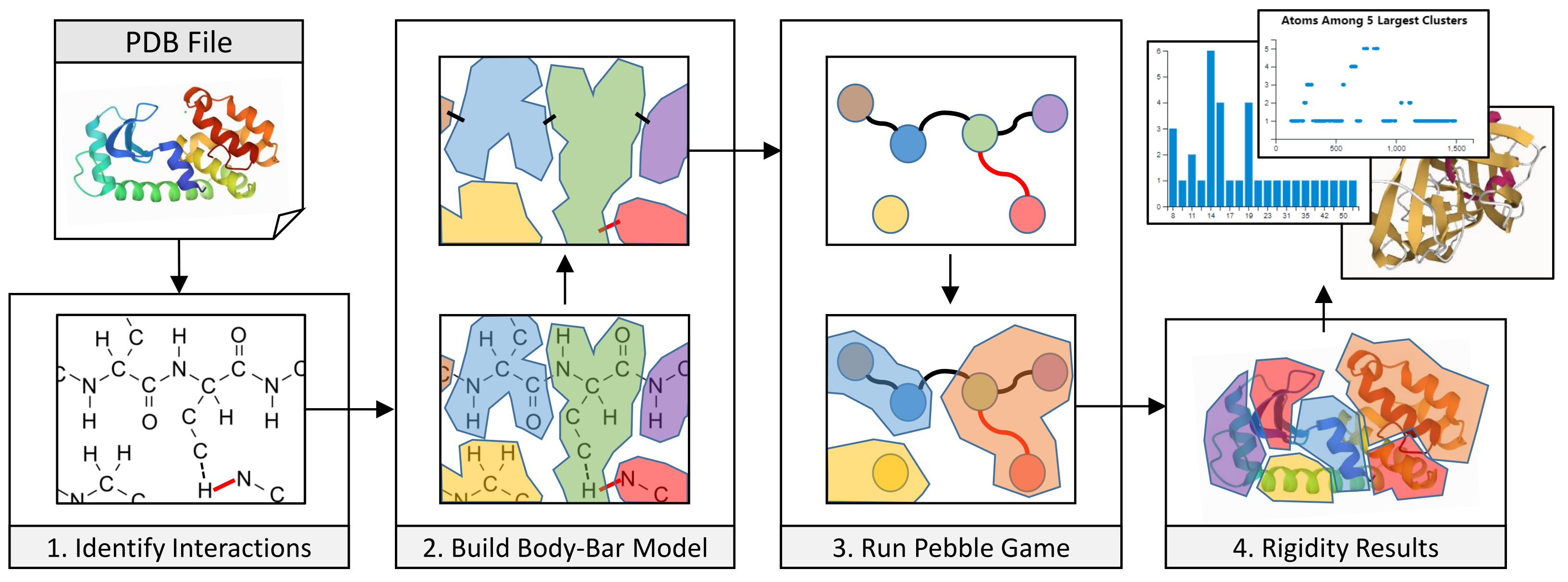
3. Methods
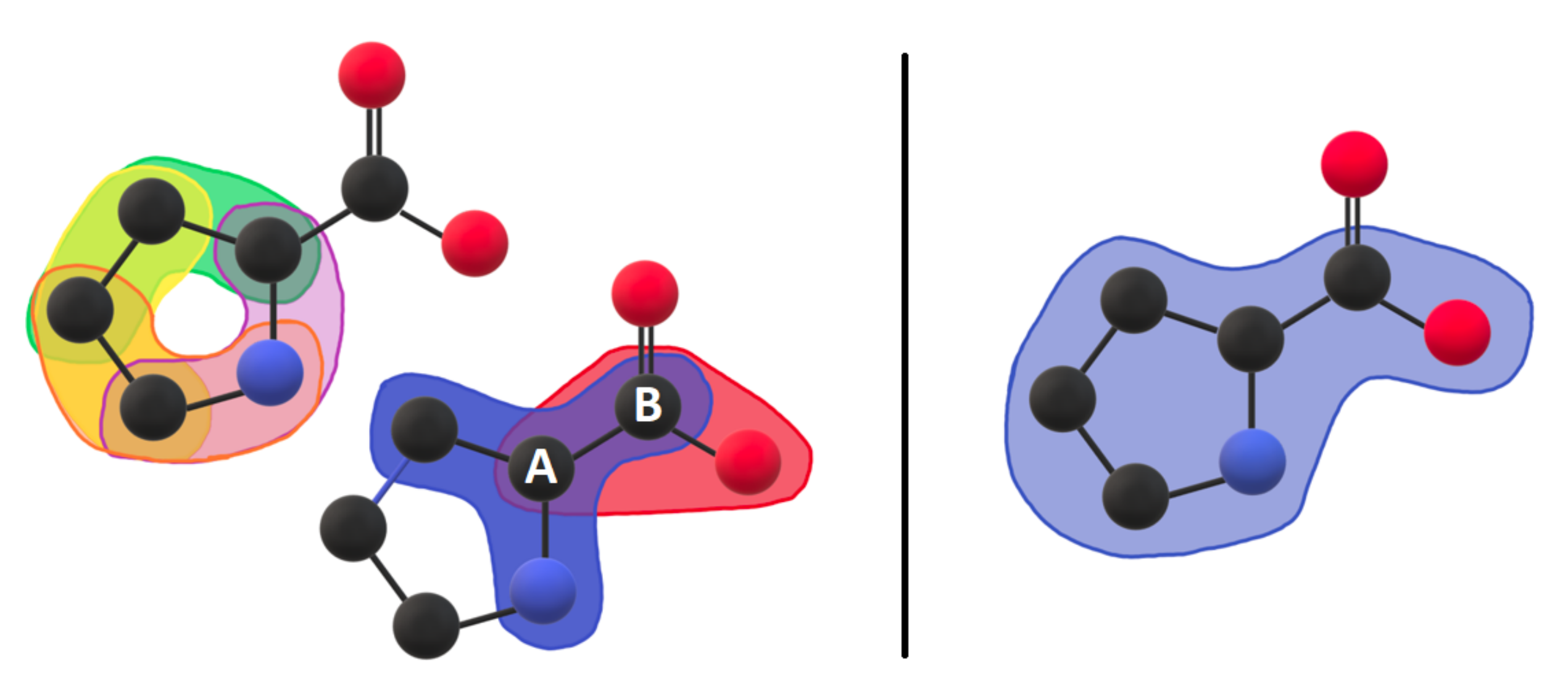
3.1. Coarse-Grained Body-Bar Mechanical Model
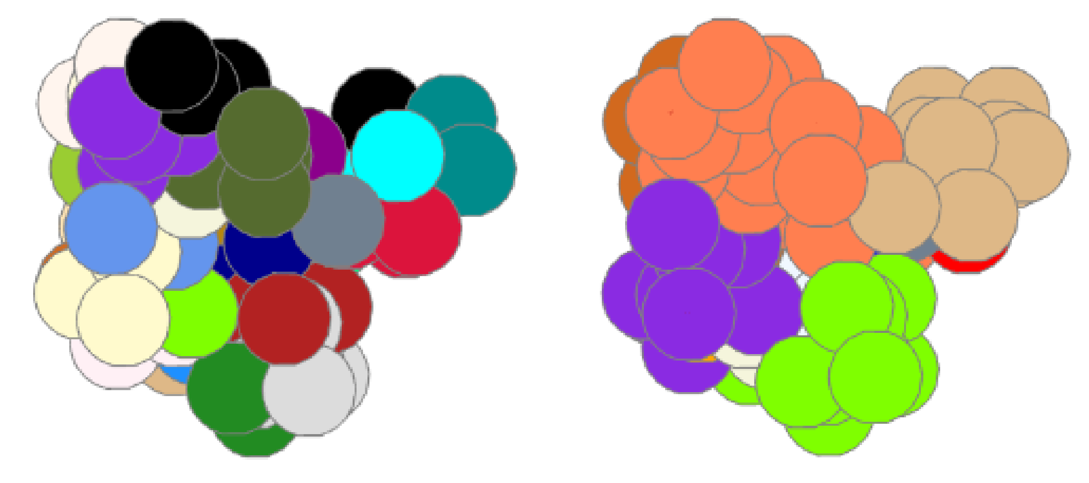
3.2. Coarse-Grained Associated Graph
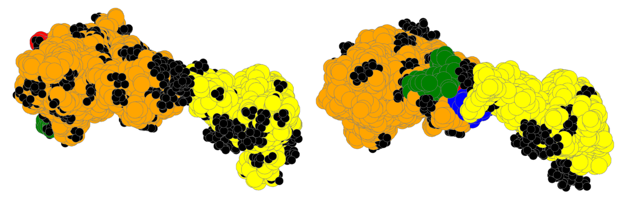
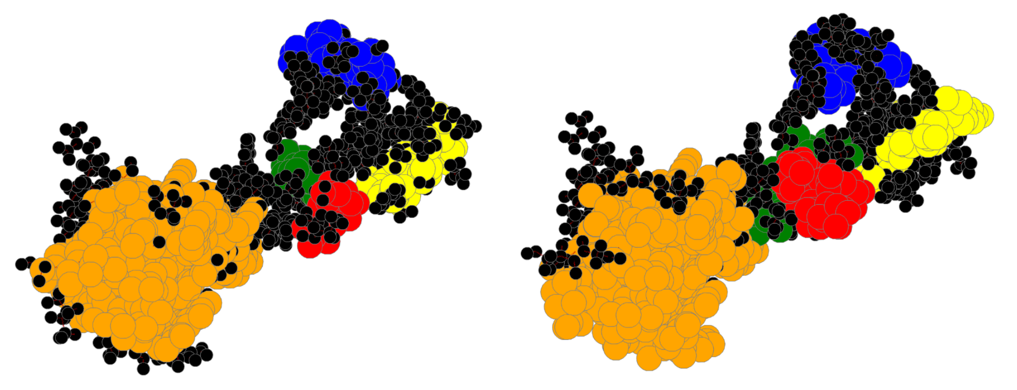
3.3. Metrics for Rigidity Analysis Comparison
3.4. Server
4. Results
4.1. Bin:
4.2. Bin:
4.3. Bin: Very Good
4.4. Bin:
4.5. Bin:
4.6. Large Proteins
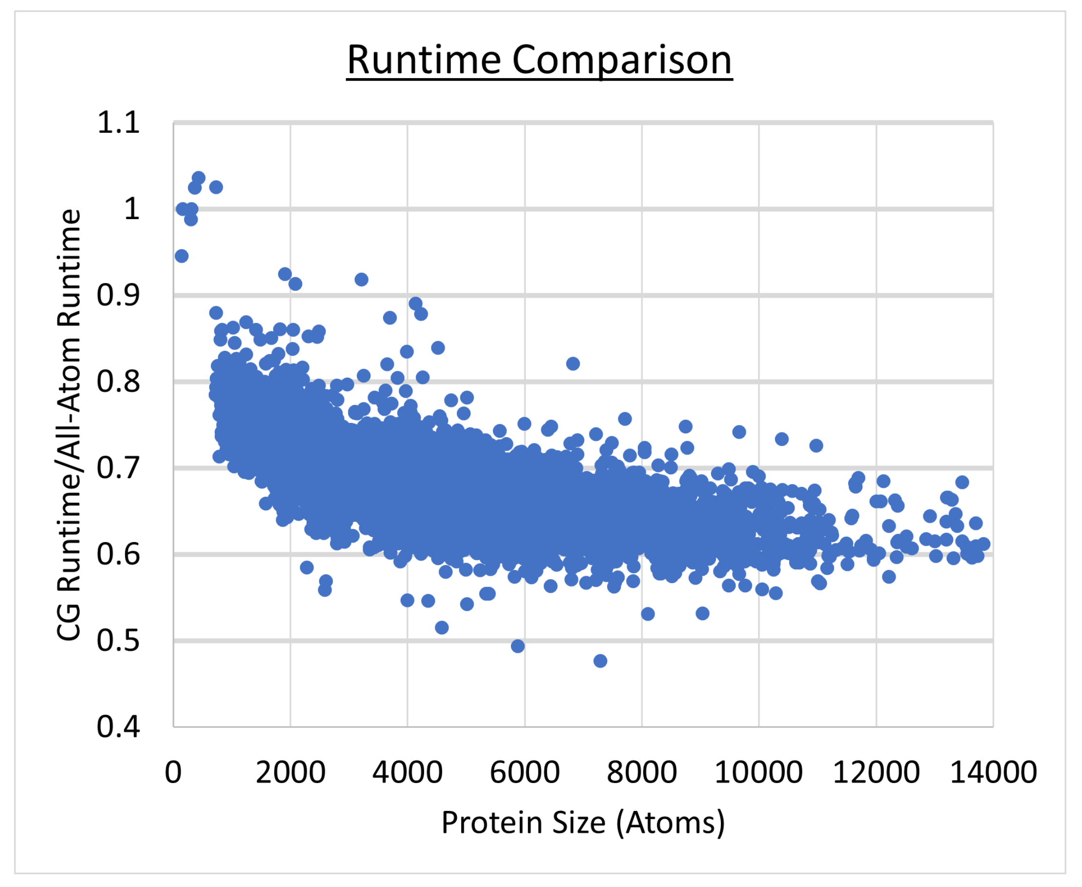
4.7. Speedup Using CGRAP
5. Discussion
6. Conclusions
Author Contributions
Funding
Institutional Review Board Statement
Informed Consent Statement
Data Availability Statement
Conflicts of Interest
References
- Xu, Y.; Havenith, M. Perspective: Watching low-frequency vibrations of water in biomolecular recognition by THz spectroscopy. J. Chem. Phys. 2015, 143, 170901. [Google Scholar] [CrossRef] [PubMed] [Green Version]
- Teague, S.J. Implications of protein flexibility for drug discovery. Nat. Rev. Drug Discov. 2003, 2, 527–541. [Google Scholar] [CrossRef]
- Bonvin, A.M. Flexible protein–protein docking. Curr. Opin. Struct. Biol. 2006, 16, 194–200. [Google Scholar] [CrossRef] [Green Version]
- Davis, A.M.; Teague, S.J.; Kleywegt, G.J. Application and limitations of X-ray crystallographic data in structure-based ligand and drug design. Angew. Chem. Int. Ed. 2003, 42, 2718–2736. [Google Scholar] [CrossRef]
- del Carmen Fernández-Alonso, M.; Díaz, D.; Alvaro Berbis, M.; Marcelo, F.; Jimenez-Barbero, J. Protein-carbohydrate interactions studied by NMR: From molecular recognition to drug design. Curr. Protein Pept. Sci. 2012, 13, 816–830. [Google Scholar] [CrossRef] [Green Version]
- Jamroz, M.; Kolinski, A.; Kmiecik, S. CABS-flex predictions of protein flexibility compared with NMR ensembles. Bioinformatics 2014, 30, 2150–2154. [Google Scholar] [CrossRef] [PubMed]
- Kubinyi, H. Combinatorial and computational approaches in structure-based drug design. Curr. Opin. Drug Discov. Dev. 1998, 1, 16–27. [Google Scholar]
- Comeau, S.R.; Gatchell, D.W.; Vajda, S.; Camacho, C.J. ClusPro: A fully automated algorithm for protein–protein docking. Nucleic Acids Res. 2004, 32, W96–W99. [Google Scholar] [CrossRef] [PubMed] [Green Version]
- Jagodzinski, F.; Hardy, J.; Streinu, I. Using rigidity analysis to probe mutation-induced structural changes in proteins. In Proceedings of the 2011 IEEE International Conference on Bioinformatics and Biomedicine Workshops (BIBMW), Atlanta, GA, USA, 12–15 November 2011; pp. 432–437. [Google Scholar] [CrossRef] [Green Version]
- Maxwell, J.C. XLV. On reciprocal figures and diagrams of forces. Lond. Edinb. Dublin Philos. Mag. J. Sci. 1864, 27, 250–261. [Google Scholar] [CrossRef]
- Laman, G. On graphs and rigidity of plane skeletal structures. J. Eng. Math. 1970, 4, 331–340. [Google Scholar] [CrossRef]
- Tay, T.S. Rigidity of multi-graphs. I. Linking rigid bodies in n-space. J. Comb. Theory Ser. B 1984, 36, 95–112. [Google Scholar] [CrossRef] [Green Version]
- Thorpe, M.F. Continuous deformations in random networks. J.-Non-Cryst. Solids 1983, 57, 355–370. [Google Scholar] [CrossRef]
- Hermans, S.M.; Pfleger, C.; Nutschel, C.; Hanke, C.A.; Gohlke, H. Rigidity theory for biomolecules: Concepts, software, and applications. Wiley Interdiscip. Rev. Comput. Mol. Sci. 2017, 7, e1311. [Google Scholar] [CrossRef]
- Lee, A.; Streinu, I. Pebble game algorithms and sparse graphs. Discret. Math. 2008, 308, 1425–1437. [Google Scholar] [CrossRef] [Green Version]
- Jacobs, D.J.; Thorpe, M.F. Generic Rigidity Percolation: The Pebble Game. Phys. Rev. Lett. 1995, 75, 4051–4054. [Google Scholar] [CrossRef]
- Li, T.; Tracka, M.B.; Uddin, S.; Casas-Finet, J.; Jacobs, D.J.; Livesay, D.R. Rigidity Emerges during Antibody Evolution in Three Distinct Antibody Systems: Evidence from QSFR Analysis of Fab Fragments. PLoS Comput. Biol. 2015, 11, e1004327. [Google Scholar] [CrossRef] [Green Version]
- Dahiyat, B.; Gordon, D.; Mayo, S. Automated design of the surface positions of protein helices. Protein Sci. Publ. Protein Soc. 1997, 6, 1333–1337. [Google Scholar] [CrossRef] [PubMed] [Green Version]
- Fox, N.; Jagodzinski, F.; Streinu, I. KINARI-Lib: A C++ library for mechanical modeling and pebble game rigidity analysis. In Proceedings of the Minisymposium on Publicly Available Geometric/Topological Software, Chapel Hill, NC, USA, 17–19 June 2012. [Google Scholar]
- McDonald, I.K.; Thornton, J.M. Satisfying Hydrogen Bonding Potential in Proteins. J. Mol. Biol. 1994, 238, 777–793. [Google Scholar] [CrossRef]
- Fox, N.; Jagodzinski, F.; Li, Y.; Streinu, I. KINARI-Web: A server for protein rigidity analysis. Nucleic Acids Res. 2011, 39, W177–W183. [Google Scholar] [CrossRef] [PubMed]
- Shehu, A.; Kavraki, L.E. Modeling structures and motions of loops in protein molecules. Entropy 2012, 14, 252. [Google Scholar] [CrossRef] [Green Version]
- Dehghanpoor, R.; Ricks, E.; Hursh, K.; Gunderson, S.; Farhoodi, R.; Haspel, N.; Hutchinson, B.; Jagodzinski, F. Predicting the effect of single and multiple mutations on protein structural stability. Molecules 2018, 23, 251. [Google Scholar] [CrossRef] [PubMed] [Green Version]
- Luo, D.; Haspel, N. Multi-resolution rigidity-based sampling of protein conformational paths. In Proceedings of the International Conference on Bioinformatics, Computational Biology and Biomedical Informatics, Washington, DC, USA, 22–25 September 2013; pp. 786–792. [Google Scholar]
- Andersson, E.; Hsieh, R.; Szeto, H.; Farhoodi, R.; Haspel, N.; Jagodzinski, F. Assessing how multiple mutations affect protein stability using rigid cluster size distributions. In Proceedings of the 2016 IEEE 6th International Conference on Computational Advances in Bio and Medical Sciences (ICCABS), Atlanta, GA, USA, 13–15 October 2016; pp. 1–6. [Google Scholar]
- Odersky, M.; Spoon, L.; Venners, B. Programming in Scala; Artima Inc.: Walnut Creek, CA, USA, 2008. [Google Scholar]
- Sehnal, D.; Bittrich, S.; Deshpande, M.; Svobodová, R.; Berka, K.; Bazgier, V.; Velankar, S.; Burley, S.K.; Koča, J.; Rose, A.S. Mol* Viewer: Modern web app for 3D visualization and analysis of large biomolecular structures. Nucleic Acids Res. 2021, 49, W431–W437. [Google Scholar] [CrossRef] [PubMed]
- Zhu, N.Q. Data Visualization with D3. js Cookbook; Packt Publishing Ltd.: Birmingham, UK, 2013. [Google Scholar]


| Bin | #Prot | RT | #A | Size | SLC | LC | TLCCS |
|---|---|---|---|---|---|---|---|
| 2133 | 66% | 5358 | 12% | 46 | 83% | 0.73 | |
| 2292 | 67% | 4847 | 20% | 68 | 80% | 0.65 | |
| very good | 1993 | 68% | 4311 | 34% | 121 | 76% | 0.56 |
| 1058 | 68% | 4227 | 69% | 295 | 72% | 0.43 | |
| 1570 | 70% | 3795 | 184% | 322 | 49% | 0.21 |
Publisher’s Note: MDPI stays neutral with regard to jurisdictional claims in published maps and institutional affiliations. |
© 2021 by the authors. Licensee MDPI, Basel, Switzerland. This article is an open access article distributed under the terms and conditions of the Creative Commons Attribution (CC BY) license (https://creativecommons.org/licenses/by/4.0/).
Share and Cite
Turcan, A.; Zivkovic, A.; Thompson, D.; Wong, L.; Johnson, L.; Jagodzinski, F. CGRAP: A Web Server for Coarse-Grained Rigidity Analysis of Proteins. Symmetry 2021, 13, 2401. https://doi.org/10.3390/sym13122401
Turcan A, Zivkovic A, Thompson D, Wong L, Johnson L, Jagodzinski F. CGRAP: A Web Server for Coarse-Grained Rigidity Analysis of Proteins. Symmetry. 2021; 13(12):2401. https://doi.org/10.3390/sym13122401
Chicago/Turabian StyleTurcan, Alistair, Anna Zivkovic, Dylan Thompson, Lorraine Wong, Lauren Johnson, and Filip Jagodzinski. 2021. "CGRAP: A Web Server for Coarse-Grained Rigidity Analysis of Proteins" Symmetry 13, no. 12: 2401. https://doi.org/10.3390/sym13122401
APA StyleTurcan, A., Zivkovic, A., Thompson, D., Wong, L., Johnson, L., & Jagodzinski, F. (2021). CGRAP: A Web Server for Coarse-Grained Rigidity Analysis of Proteins. Symmetry, 13(12), 2401. https://doi.org/10.3390/sym13122401