Multi-Objective Optimization of Differentiated Urban Ring Road Bus Lines and Fares Based on Travelers’ Interactive Reinforcement Learning

Abstract

This paper proposes a new multi-objective bi-level programming model for the ring road bus lines and fare design problems. The proposed model consists of two layers: the traffic management operator and travelers. In the upper level, we propose a multi-objective bus lines and fares optimization model in which the operator’s profit and travelers’ utility are set as objective functions. In the lower level, evolutionary multi agent model of travelers’ bounded rational reinforcement learning with social interaction is introduced. A solution algorithm for the multi-objective bi-level programming is developed on the basis of the equalization algorithm of OD matrix. A numerical example based on a real case was conducted to verify the proposed models and solution algorithm. The computational results indicated that travel choice models with different degrees of rationality significantly changed the optimization results of bus lines and the differentiated fares; furthermore, the multi-objective bi-level programming in this paper can generate the solution to reduce the maximum section flow, increase the profit, and reduce travelers’ generalized travel cost.

1. Introduction

1.1. Background and Motivation

In recent years, with the continuous increase of the scale of big cities, the road network of many large cities presents a ring structure spreading from the center to the periphery. From the perspective of urban planning, in cities with high population density, the ring road plays an important role in alleviating congestion in urban centers and realizing rapid connectivity between urban areas [1]. The ring road traffic congestion index should show the characteristics of gradually decreasing from the core area to the periphery, and according to the Beijing Transportation Development Annual Report 2021, the traffic congestion index in Beijing has decreased under the COVID-19 virus situation; however, congestion still occurs frequently in some ring roads. For example, during the rush hour of public transportation, there has been a long period of congestion between Ciyunsi bridge and Dajiaoting bridge on the middle east fourth ring road, which indicates that the bus line operation on the ring road needs to be further optimized.

In addition, in the existing research of traffic flow evolution and travel behavior, scholars have carried out some important research on the endogenous complexity of travel behavior, such as traveler’s reference point dependency, psychological account, regret aversion, and social interaction [2,3]. Through these studies, scholars found that, under the influence of bounded rationality, social interaction, and behavioral complexity, the traffic flow evolution is affected by the complexity of group decision making. Therefore, the design and operation scheme of bus lines will also be affected by the complexity of travelers’ group behavior in terms of traffic system optimization, the impact of travelers’ bounded rationality, social interaction, and daily evolutionary complexity on the optimization results of the transportation system, which deserves more in-depth research.

1.2. Literature Review

The optimization of bus line operation seeks to facilitate people’s traveling by adjusting the existing stop schedule plan, differentiated fares, timetable, etc. In general, the objective function contains profit maximization, maximizing travel utility, minimizing the operation cost, etc. In recent years, more and more studies have found that optimizing the variables related to travel behavior or utility can significantly improve the performance of traffic system. Hm et al. [4] found that optimizing the timetable on the basis of the dynamic travel demand of passengers can effectively increase the line passenger flow. On the basis of the multi-source big data, Yu et al. [5] accurately extracted candidate stations, which are very popular with travelers and convenient for transfer; the empirical study of a real case showed that the optimized lines can quickly satisfy travelers’ demand. Aiming at minimizing the cost of travelers and operators, Liang et al. [6] established a multi-objective optimization model of bus networks, which successfully reduced travelers’ waiting time and the in-vehicle time. Aiming at the optimization problem of bus network with demand response and the revenue of operators, Huang et al. [7] proposed a two-stage (static phase and dynamic phase) optimization model to solve the network design problem. Zhang et al. [8] introduced the travel time dependence of travelers into the bus timetable optimization problem, significantly improving the utility of passengers.

On the other hand, some studies in recent years have also found that, in addition to reasonable bus line design, the differentiated fares can also improve the efficiency of the traffic system; compared with the traditional fare scheme, differentiated bus fares strategy often has more advantages [9,10]. The differentiated fares system can effectively reduce travelers’ time cost and alleviate traffic congestion during peak hours [11,12]. The implementation of differentiated fares based on comfort level can reduce social costs and is more conducive to the public transport system than charging congestion fees [13]. In addition, the differentiated bus fares scheme can achieve a better balance between eliminating externalities and ensuring consumer surplus, as well as improving the Pareto distribution [12,13].

From the above literature review, it can be seen that the joint improvement and optimization of bus network and fare scheme can effectively improve the efficiency of transportation system. However, the research on the joint optimization of bus network and differentiated fares need to be further deepened; moreover, most of the existing studies of bus lines and fares have some basic assumptions, such as simplifying travelers’ behavior factors, but the cluster behavior of travelers is usually not considered. Some typical studies have found that after the implementation of the optimization scheme, there will still be a social dilemma [14,15] in the use of transportation resources. This is because, on the one hand, the traffic system is a typical complex socio-economic system; travelers’ decision making will be affected by social environment and bounded rationality [16]; and under the influence of multi-channel information, cluster travel behavior has the characteristics of learning and interaction [17,18]. On the other hand, travel choice is a day-to-day evolution process [19], and thus there is an uncertain causal relationship between travelers’ traffic information and behavior [20]. In addition, it is very difficult for travelers to accurately obtain the utility information of all potential travel modes, and thus it is also difficult to simulate the process of travel experience accumulation by using the analytical model.

The work of this paper is mainly divided into two parts: firstly, travelers’ reinforcement learning with social interaction is introduced into the ring road bus lines design problem. Secondly, a multi-objective bi-level programming of bus lines and differentiated ticket fares joint optimization model is established, and the solution algorithm in which the swarm intelligence multi-objective optimization algorithm is combined with the equalization algorithm of OD matrix is designed. Moreover, the model we proposed in this paper was applied to the Fourth Ring Road in Beijing to verify the effectiveness of the model.

1.3. Paper Organization

The remainder of this paper is organized as follows. The problem statement and basic assumptions are presented in Section 2. The analysis of generalized travel cost is presented in Section 3. Section 4 describes travelers’ BM reinforcement learning model with social interaction, which is followed by the properties of the model. Section 5 proposes the multi-objective bi-level programming model of bus lines and differentiated ticket fares, and Section 6 presents the corresponding solution algorithm of multi-objective bi-level programming. Section 7 presents the numerical example under real case to verify the proposed model and algorithm. Section 8 concludes this paper.

2. Problem Statement and the Basic Assumptions

2.1. Problem Statement

Consider a graph $G=\left(V,A\right)$ of urban ring road that contains $N$ main bus stops, where $V$ is the set of bus stop and $A$ is the set of links ($a\in A$). Let $R$ denote the set of ring bus lines, where each bus line is composed of bus stops and links, and let $p$ denote the travel mode of private car and $b$ the travel mode of shared bike. Let $\mathbf{D}=\left(\begin{array}{ccc}{D}_{1,1}& \cdots & D_{1,N}\\ ⋮& & ⋮\\ D_{N,1}& \cdots & D_{N,N}\end{array}\right)$ denote the demand matrix in graph $G$, in which $D_{i,j}$ represents the travel demand between bus stop $i$ and $j$. In the ring road, travelers always choose the shortest route, in daily travel activities, travelers can choose buses, private car, and shared bike between OD $i$ and $j$; thus, $D_{i,j}^r$ is the travel demand of bus line $r$ between OD $i$ and $j$. Due to the competition between different travel modes and travelers’ option between different bus lines on the ring road, the traffic flow will transfer among different ring bus lines, private cars, and shared bike.

In reality, there are often different stop schedule plans for different ring bus lines on the ring road; let $N_{\max }^{line}$ denote the maximum number of ring bus lines on the ring road. Thus, the stop schedule plans can be represented as a 0–1 matrix (see

Table 1. The matrix of stop schedule plans.

	Bus Stop 1	Bus Stop 2	Bus Stop i	Bus Stop N
Bus line 1	1	1	1	1
Bus line 2	0	1	0	1
Bus line k	1	1	1	0
$\mathrm{Bus} \mathrm{line} N_{\max }^{line}$	0	0	1	1

):

It can be seen from Table 1 that in the matrix, “1” represents the fact that the bus will stop here, and “0” represents the fact that the bus will not stop here. In addition, there are differentiated ticket fares $P_r$ per kilometer for the $N_{\max }^{line}$ bus lines; if travelers choose private car or shared bike, they will have to pay the parking fee or bike sharing fee. The objective of the bus operation management department is to optimize and adjust the stop schedule plans and differentiated fares of bus lines, so as to improve the operation income, expand social welfare, and balance the transportation resources. Therefore, in this paper, we set the matrix of stop schedule plans and differentiated fares of bus lines as the optimization variables.

2.2. Basic Assumptions

(1)

Travel demand between bus stops. The travel demand D between bus stops is obtained from real daily bus IC card data in Beijing.

(2)

Travelers’ bounded rationality. It is difficult for travelers to know the accurate utility information of all potential travel modes at the same time. Travel decision-making is affected by travel cost, information interaction, and historical travel experience; thus, travelers’ perception of utility is a process of reinforcement learning.

(3)

Travel modes. There are three optional travel modes among bus stops: (1) buses, (2) private car, and (3) shared bike. In the ring bus lines, travelers can travel between any two bus stops without changing lines, and they always choose the shortest path (in a ring bus line, there are clockwise and counterclockwise paths from bus stop i to bus stop j). Let d^* denote the critical distance of bicycle riding; when the distance between OD is larger than d^*, travelers will not choose to ride a bicycle (Figure 1).

3. Generalized Travel Cost

By summarizing the literature on travel behavior, we find that the generalized travel cost consists of the following elements:

(1)

Psychological time of waiting the bus

For travelers who choose buses, they arrive at the bus stop in the Poisson process with the intensity of $\lambda$; let ${\varphi }_r$ denote the departure frequency of bus line $r$, let ${\tau }_x$ denote the time of traveler $x$’s arrival at the bus stop, and the arrival of travelers can be regarded as independent random variables which obey the uniform distribution on the interval $[0,\frac{1}{{\varphi }_r}]$. Thus, we have $E\left({\tau }_x\right)=\frac{1}{2{\varphi }_r}$, and the waiting time can be represented as $\frac{1}{{\varphi }_r}-{\tau }_x$. Let $S\left(\tau \right)$ denote the number of travelers arriving at the bus stop at time $\tau$, and thus the expected waiting time of travelers can be formulated as $E\left[{\displaystyle \sum _{x=1}^{S\left(\tau \right)}\left(\frac{1}{{\varphi }_r}-{\tau }_x\right)}\right]$. According to the time processing theory, there is a certain difference between travelers’ psychological feeling and the actual physical time, and the psychological feeling is more in accordance with travelers’ perception of utility. Therefore, the physical time should be converted into psychological time $\alpha {\left(\frac{1}{{\varphi }_r}-{\tau }_x\right)}^{\beta }$, and $\alpha$ and $\beta$ represent travel purpose coefficient and attention coefficient, respectively. Moreover, we have

$$\{\begin{array}{l}{E}_{psy}\left[{{\displaystyle \sum _{x=1}^{S\left(\tau \right)}\alpha \left(\frac{1}{{\varphi }_r}-{\tau }_x\right)}}^{\beta }\right]=\lambda {{\displaystyle {\int }_0^{\tau }\alpha \left(\frac{1}{{\varphi }_r}-{\tau }_x\right)}}^{\beta }d{\tau }_x\\ E\left[S\left(\tau \right)\right]=\frac{\lambda }{{\varphi }_r}\end{array}$$

(1)

Solve Equation (1), and travelers’ psychological time of waiting the bus can be formulated as $T_{psy}^r=\frac{\alpha }{{\varphi }_r^{\beta }\left(\beta +1\right)}$; for the travelers who choose private car and shared bike, their psychological time of waiting is 0.

(2)

Travel time

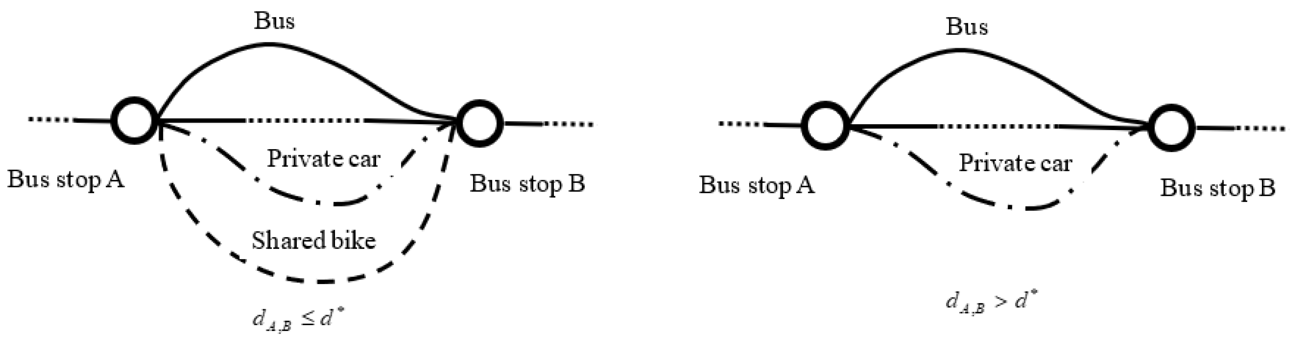
For travelers who choose buses between OD $i,j$ on day $t$, if they choose the bus line $r$, the travel time can be represented as $T_{i,j}^{r,t}$. For travelers who choose private cars, in this paper, we assume that the travel time of private car between OD $i,j$ equals the shortest bus line travel time, which can be represented as $T_{i,j}^{p,t}=\underset{r\in R}{\min }\left\{T_{i,j}^{r,t}\right\}$. For travelers who choose shared bike, the travel time between OD $i,j$ is $T_{i,j}^{b,t}=\frac{d_{i,j}}{v_b}$, in which $d_{i,j}$ is the distance between bus stop $i$ and $j$, and $v_b$ is the average speed of a bicycle.

(3)

Crowding degree

For travelers who choose buses, due to the restrictions of bus capacity and different stop schedule plans, the bus will be crowded; take bus line $r$ which contains $N_r$ bus stops for instance, and let $f_{i,i+1}^{r+,t}$ and $f_{i,i+1}^{r-,t}$ represent the up direction (from $i$ to $i+1$) and down direction (from $i+1$ to $i$) traffic flow between bus stop $i$ and $i+1$ on day $t$, respectively. Thus, we have

$$\{\begin{array}{l}{f}_{i,i+1}^{r+,t}=f_{i-1,i}^{r+,t}+{\displaystyle \sum _{j=i}^{N_r}{D}_{i,j}^{r,t}}-{\displaystyle \sum _{j=1}^i{D}_{j,i}^{r,t}}\\ f_{i,i+1}^{r-,t}=f_{i+1,i+2}^{r-,t}+{\displaystyle \sum _{j=1}^{i+1}{D}_{i+1,j}^{r,t}}-{\displaystyle \sum _{j=i+1}^{N_r}{D}_{j,i+1}^{r,t}}\end{array}$$

(2)

Then the maximum section flow is $\max \left\{f_{i,i+1}^{r+}+f_{i,i+1}^{r-}\right\}\left(r\in R,i\in V\right)$, and the crowding degree of bus line $r$ between bus stop $i$ and $j$ on day $t$ can be formulated as

$$\{\begin{array}{l}{C}_{i,j}^{r+,t}={\displaystyle \sum _{s=i}^{j-1}\frac{\eta f_{s,s+1}^{r+,t}}{V^r\cdot {\varphi }_r}}\\ C_{i,j}^{r-,t}={\displaystyle \sum _{s=i}^{j-1}\frac{\eta f_{s,s+1}^{r-,t}}{V^r\cdot {\varphi }_r}}\end{array}$$

(3)

Here, $V^r$ represents the bus capacity of line $r$, and $\eta$ is crowding factor. In addition, we assume that the crowding degree (not traffic jam) of private car and shared bike is 0.

(4)

Bus ticket fare, parking fee of private car, and bike sharing fee

For travelers who choose buses, let $P_r$ denote the fare per kilometer of bus line $r$; thus, travelers need to pay $P_r\cdot d_{i,j}$. For travelers who choose private car and shared bike, they need to pay the parking fee and bike sharing fee, which are represented as ${\tilde{P}}_p$ and ${\tilde{P}}_b$.

(5)

The effect of social interaction on travel cost

Let ${\xi }_x=1$ denote traveler $x$ chooses bus, and ${\xi }_x=-1$ represents traveler $x$ chooses other travel modes, while ${\lambda }_m$ is social interaction level. Let $E\left({\mu }_x\right)$ denote traveler’s expectation of travel mode choice between bus stop $i$ and $j$; thus, $E\left({\mu }_x\right)=\frac{{\displaystyle \sum _{y\ne x}E\left({\mu }_y\right)}}{{\overline{D}}_{i,j}-1}$, and according to the principle of multiplier interaction, the effect of social interaction on day $t$ can be formulated as

$$M_{i,j}^t\left({\xi }_x,{\mu }_x\right)=\frac{{\lambda }_m\cdot {\xi }_x\cdot {\displaystyle \sum _{y\ne x}E\left({\mu }_y\right)}}{{\overline{D}}_{i,j}-1}$$

(4)

In summary, the generalized travel cost between bus stop $i$ and $j$ on day $t$ can be formulated as

$$\{\begin{array}{l}{G}_{i,j}^{\kappa ,t}={\zeta }_{psy}\cdot T_{psy}^{\kappa }+{\zeta }_T\cdot T_{i,j}^{\kappa ,t}+{\zeta }_C\cdot C_{i,j}^{\kappa ,t}+{\zeta }_P\cdot P_{\kappa }\cdot d_{i,j}+{\zeta }_M\cdot M_{i,j}^t\left({\xi }_x,{\mu }_x\right),\left(\kappa =r,r\in R\right)\\ G_{i,j}^{\kappa ,t}={\zeta }_T\cdot T_{i,j}^{\kappa ,t}+{\zeta }_C\cdot C_{i,j}^{\kappa ,t}+{\zeta }_P\cdot {\tilde{P}}_{\kappa }+{\zeta }_M\cdot M_{i,j}^t\left({\xi }_x,{\mu }_x\right),\left(\kappa =p,b\right)\end{array}$$

(5)

Here, ${\zeta }_{psy}$, ${\zeta }_T$, ${\zeta }_C$, ${\zeta }_P$, ${\zeta }_M$ represent cost coefficients.

In the existing studies, some scholars use the social interaction model to simulate group travel choice behavior, but in reality, the essence of “interaction” is the diffusion of asymmetric and incomplete travel information in the group. Travelers make decisions based on the external information they receive, rather than being directly influenced by other travelers’ behavior. Therefore, in this paper, travelers’ social interaction is reflected in the information of generalized travel cost (Equation (5)) rather than the choice behavior itself.

4. BM Reinforcement Learning Model with Interaction

In real travel activities, travelers’ behavior is not always completely rational, and counterintuitive paradox often occurs in daily travel choice decision making, which conflicts with the traditional expected utility theory. In recent years, regret theory has been developed continuously. Regret theory holds that the decision making of travelers’ route (travel mode) choice is not only related to the utility of the selected route itself, but also related to the feedback generated by the comparison with other alternative routes (travel modes). At present, regret theory has been found to be more accurate in describing travelers’ decision-making behavior in an uncertain environment, and the calculated results are more in accordance with the reality. Therefore, this paper describes travelers’ generalized cost according to regret theory.

4.1. Utility Based on Regret Theory

The model construction of regret theory has experienced the improvement process from RRM1 [21] to RRM2 [22], and then to the consideration of path impedance and “regret feeling” [23]. In this paper, the construction idea of the regret theory is organically combined with the above travel scenarios, and the travel mode choice model is constructed as follows.

The regret cost based on generalized travel cost is formulated as

$${\overline{h}}_{i,j}^{\kappa ,t}=G_{i,j}^{\kappa ,t}-\delta \left(\underset{\kappa \in \left\{R,p,b\right\}}{\min }\left\{{G^{\prime }}_{i,j}^{\kappa ,t}\right\}-{G^{\prime }}_{i,j}^{\kappa ,t}\right)$$

(6)

The formation of regret psychology is based on the objective generalized cost observed by travelers; thus, we use ${G^{\prime }}_{i,j}^{\kappa ,t}$ to represent the generalized travel cost without social interaction. According to the design method of regret function, the function $\delta \left(x^{\prime }\right)$ can be represented as

$$\delta \left(x\right)=1-e^{-\psi \cdot x^{\prime }}$$

(7)

Here, $\psi$ represents travelers’ regret aversion level; the larger the value of $\psi$, the more regret-averse the traveler is.

Furthermore, in this paper, we assume that travelers’ regret aversion level $\psi$ is heterogeneous. Let $N_{agent}$ be the number of agents participating in the reinforcement learning simulation between each OD pair; $N_{agent}$ agents form the decision space ${\mathsf{\Omega }}_{agent}$ ($x\in {\mathsf{\Omega }}_{agent}$), and agents are distributed in the grid, with each node representing a traveler. After the traveling between bus stop $i$ and $j$ on day $t$, each traveler would like to update their $\psi$ through information exchanging in the Moore neighborhood (unlike the travel information on various intelligent devices, regret aversion is an endogenous psychological activity, and thus we set a small interaction range).

This process can be designed as follows:

(1) Each traveler $x$ chooses the traveler with the lowest regret cost in the neighborhood (denoted as $x^{\ast }$).

$${\overline{h}}_{i,j,x^{\ast }}^{\kappa ,t}=\min \left\{{\overline{h}}_{i,j,x}^{\kappa ,t}|x\in {\mathsf{\Omega }}_{neighbor}\right\}$$

(8)

(2) Let ${\psi }_{x^{\ast }}$ be the regret aversion level of traveler $x^{\ast }$, and traveler $x$ updates their value of ${\psi }_x$ with the intensity of $p_c$.

$${\psi }_x^{t+1}=\left(1-p_c\right)\cdot {\psi }_x^t+p_c\cdot {\psi }_{x^{\ast }}^t$$

(9)

4.2. Bush–Mosteller Reinforcement Learning Model Based on Regret Theory

Most of the existing studies use logit model to depict the choice of travel mode, in which travelers know exactly the utility of each potential choice when making decisions. However, in reality, it is difficult for travelers to know the accurate utility information of all potential choices, and travelers’ choice of travel mode is a process of continuous improvement of their own experience that is affected by travel cost, information interaction, and historical travel experience. Therefore, in this paper, the Bush–Mosteller reinforcement learning model is introduced to simulate the evolution process of travelers’ travel mode choice.

Traveler $x$ can only choose one single travel mode in one day, and they may choose different travel modes in a few days, which indicates that in a long period of daily travel activities, travelers can not only obtain the perceptive utility (PU) of every travel mode but can also gain the experience of travel mode utility (EU) on day $t$. Let $U_{i,j}^{\kappa ,t}$ and $E_{i,j}^t$ denote the PU of travel mode $\kappa$ and the EU on day $t$, respectively, which can be formulated as

$$U_{i,j,x}^{\kappa ,t}=\{\begin{array}{l}\frac{{\displaystyle {\sum }_{s=1}^t\left(-{\overline{h}}_{i,j,x}^{\kappa ,t}\right)\cdot {\epsilon }_{i,j,x}^{\kappa ,s}}}{{\displaystyle {\sum }_{s=1}^t{\epsilon }_{i,j,x}^{\kappa ,s}}},s\le L\\ \frac{{\displaystyle {\sum }_{s^{\prime }=t-L}^t\left(-{\overline{h}}_{i,j,x}^{\kappa ,t}\right)\cdot {\epsilon }_{i,j,x}^{\kappa ,s}}}{{\displaystyle {\sum }_{s=t-L}^t{\epsilon }_{i,j,x}^{\kappa ,s}}},s>L\end{array}$$

(10)

$$E_{i,j,x}^t=\{\begin{array}{l}\frac{{\displaystyle {\sum }_{s=1}^{t-1}\left(-{\overline{h}}_{i,j,x}^{\kappa ,t}\right)}}{t-1},s\le L\\ \frac{{\displaystyle {\sum }_{s=t-L}^{t-1}\left(-{\overline{h}}_{i,j,x}^{\kappa ,t}\right)}}{t-L},s>L\end{array}$$

(11)

Here, ${\epsilon }_{i,j,x}^{\kappa ,s}$ is the 0–1 variable; if traveler $x$ chooses the travel mode $\kappa$ between bus stop $i$ and $j$ on day $t$, then ${\epsilon }_{i,j,x}^{\kappa ,s}=1$, or else ${\epsilon }_{i,j,x}^{\kappa ,s}=0$. $L$ represents traveler’s memory length of historical regret cost.

On day $t$, traveler $x$ will make a comparison between $U_{i,j,x}^{\kappa ,t}$ and $E_{i,j,x}^t$:

$$u_{i,j,x}^{\kappa ,t}=\{\begin{array}{l}\frac{U_{i,j,x}^{\kappa ,t}-E_{i,j,x}^t}{\left|\max \left\{U_{i,j,x}^{\kappa ,t}-E_{i,j}^{x,t}\right\}\right|},U_{i,j,x}^{\kappa ,t}\ge E_{i,j,x}^t\\ \frac{U_{i,j,x}^{\kappa ,t}-E_{i,j,x}^t}{\left|\min \left\{U_{i,j,x}^{\kappa ,t}-E_{i,j}^{x,t}\right\}\right|},U_{i,j,x}^{\kappa ,t}<E_{i,j,x}^t\end{array}$$

(12)

Let $l$ denote the learning intensity of travelers; traveler $x$ updates the choice probability of travel mode $\kappa$ (represented as ${\omega }_{i,j,x}^{\kappa ,t}$) and the choice probabilities of other travel modes $\neg \kappa$ (represented as ${\omega }_{i,j,x}^{-\kappa ,t}$) between bus stop $i$ and $j$.

$${\omega }_{i,j,x}^{\kappa ,t}=\{\begin{array}{l}{\omega }_{i,j,x}^{\kappa ,t-1}+\left(1-{\omega }_{i,j,x}^{\kappa ,t-1}\right)\cdot l\cdot u_{i,j,x}^{\kappa ,t-1},u_{i,j,x}^{\kappa ,t-1}\ge 0\\ {\omega }_{i,j,x}^{\kappa ,t-1}+{\omega }_{i,j,x}^{\kappa ,t-1}\cdot l\cdot u_{i,j,x}^{\kappa ,t-1},u_{i,j,x}^{\kappa ,t-1}<0\end{array}$$

(13)

$${\omega }_{i,j,x}^{\neg \kappa ,t}=\{\begin{array}{l}{\omega }_{i,j,x}^{\neg \kappa ,t-1}-{\omega }_{i,j,x}^{\neg \kappa ,t-1}\cdot l\cdot u_{i,j,x}^{\kappa ,t-1},u_{i,j,x}^{\kappa ,t-1}\ge 0\\ {\omega }_{i,j,x}^{\neg \kappa ,t-1}-\frac{{\omega }_{i,j,x}^{\neg \kappa ,t-1}\cdot {\omega }_{i,j,x}^{\kappa ,t-1}\cdot l\cdot u_{i,j,x}^{\kappa ,t-1}}{1-{\omega }_{i,j,x}^{\kappa ,t-1}},u_{i,j,x}^{\kappa ,t-1}<0\end{array}$$

(14)

The average choice probability between bus stop $i$ and $j$ can be represented as $\left({\overline{\omega }}_{i,j,x}^{\kappa ,t},{\overline{\omega }}_{i,j,x}^{-\kappa ,t}\right)$, and the traffic flow of travel mode $\kappa$ between bus stop $i$ and $j$ is $Q_{i,j}^{\kappa ,t}=D_{ij}\cdot {\overline{\omega }}_{i,j,x}^{\kappa ,t}$.

4.3. Properties of the Model

Theorem 1. 

There exists the equilibrium state of traffic flow among all the bus stops. The necessary and sufficient condition for the non-zero traffic flow of each travel mode to reach the equilibrium state is that the perceptive utility (PU) of each travel mode is the same as the experience of travel mode utility (EU), which can be formulated as

$${\displaystyle \sum _{x=1}^{Q_{ij}}{U}_{i,j,x}^{\kappa }\left({\psi }_x\right)}={\displaystyle \sum _{x=1}^{Q_{ij}}{E}_{i,j,x}\left({\psi }_x\right)},\kappa \in \left\{R,p,b\right\}$$

(15)

Proof. 

On day $t$, travelers between bus stop $i$ and $j$ can be divided into two groups, travelers who choose travel mode $\kappa$ from the first group, and travelers who do not choose travel mode $\kappa$ from the second group. For travelers from the first group, they make decisions based on Equation (13), and the probability updating formula of choosing travel mode $\kappa$ can be formulated as

$$\mathsf{\Delta }{\omega }_{i,j,x}^{\kappa ,t}=\frac{{\omega }_{i,j,x}^{\kappa ,t}-{\omega }_{i,j,x}^{\kappa ,t-1}}{{\omega }_{i,j,x}^{\kappa ,t-1}}=\{\begin{array}{l}\frac{\left(1-{\omega }_{i,j,x}^{\kappa ,t-1}\right)\cdot l\cdot u_{i,j,x}^{\kappa ,t-1}}{{\omega }_{i,j,x}^{\kappa ,t-1}},u_{i,j,x}^{\kappa ,t-1}\ge 0\\ l\cdot u_{i,j,x}^{\kappa ,t-1},u_{i,j,x}^{\kappa ,t-1}<0\end{array}$$

(16)

For travelers from the second group, they make decision based on Equation (13), and the probability updating formula of choosing travel mode $\kappa$ can be formulated as

$$\mathsf{\Delta }{\omega }_{i,j,x}^{\kappa ,t}=\{\begin{array}{l}-l\cdot u_{i,j,x}^{\neg \kappa ,t-1},u_{i,j,x}^{\neg \kappa ,t-1}\ge 0\\ -\frac{{\omega }_{i,j,x}^{\neg \kappa ,t-1}\cdot l\cdot u_{i,j,x}^{\neg \kappa ,t-1}}{1-{\omega }_{i,j,x}^{\neg \kappa ,t-1}},u_{i,j,x}^{\neg \kappa ,t-1}<0\end{array}$$

(17)

Therefore, the probability updating formula of choosing travel mode $\kappa$ for all the travelers between bus stop $i$ and $j$ can be represented as

$$\begin{array}{l}{\displaystyle \sum _{x=1}^{D_{ij}}\mathsf{\Delta }{\omega }_{i,j,x}^{\kappa }}={\displaystyle \sum _{x=1}^{Q_{i,j}^{\kappa }}\mathsf{\Delta }{\omega }_{i,j,x}^{\kappa }}+{\displaystyle \sum _{\neg \kappa \in \left\{R,p,b\right\}}{\displaystyle \sum _{x=1}^{Q_{i,j}^{\neg \kappa }}\mathsf{\Delta }{\omega }_{i,j,x}^{\kappa }}}\\ =\{\begin{array}{l}{\displaystyle \sum _{x=1}^{Q_{i,j}^{\kappa }}\frac{\left(1-{\omega }_{i,j,x}^{\kappa }\right)\cdot l\cdot u_{i,j,x}^{\kappa }}{{\omega }_{i,j,x}^{\kappa }}}-{\displaystyle \sum _{\neg \kappa \in \left\{R,p,b\right\},u_{i,j,x}^{\neg \kappa ,t-1}\ge 0}{\displaystyle \sum _{x=1}^{Q_{i,j}^{\neg \kappa }}l\cdot u_{i,j,x}^{\neg \kappa }}}-{\displaystyle \sum _{\neg \kappa \in \left\{R,p,b\right\},u_{i,j,x}^{\neg \kappa ,t-1}<0}{\displaystyle \sum _{x=1}^{Q_{i,j}^{\neg \kappa }}\frac{{\omega }_{i,j,x}^{\neg \kappa }\cdot l\cdot u_{i,j,x}^{\neg \kappa }}{1-{\omega }_{i,j,x}^{\neg \kappa }}}},u_{i,j,x}^{\kappa }\ge 0\\ {\displaystyle \sum _{x=1}^{Q_{i,j}^{\kappa }}l\cdot u_{i,j,x}^{\kappa }}-{\displaystyle \sum _{\neg \kappa \in \left\{R,p,b\right\},u_{i,j,x}^{\neg \kappa ,t-1}\ge 0}{\displaystyle \sum _{x=1}^{Q_{i,j}^{\neg \kappa }}l\cdot u_{i,j,x}^{\neg \kappa }}}-{\displaystyle \sum _{\neg \kappa \in \left\{R,p,b\right\},u_{i,j,x}^{\neg \kappa ,t-1}<0}{\displaystyle \sum _{x=1}^{Q_{i,j}^{\neg \kappa }}\frac{{\omega }_{i,j,x}^{\neg \kappa }\cdot l\cdot u_{i,j,x}^{\neg \kappa }}{1-{\omega }_{i,j,x}^{\neg \kappa }}}},u_{i,j,x}^{\kappa }<0\end{array}\end{array}$$

(18)

Moreover, combine and expand Equation (17)

$${\displaystyle \sum _{x=1}^{D_{ij}}\mathsf{\Delta }{\omega }_{i,j,x}^{\kappa }}=\{\begin{array}{l}{l}_1\cdot \left\{\begin{array}{l}{\displaystyle \sum _{x=1}^{Q_{i,j}^{\kappa }}\frac{\left[U_{i,j,x}^{\kappa }\left({\psi }_x\right)-E_{i,j,x}\left({\psi }_x\right)\right]}{{\omega }_{i,j,x}^{\kappa }}}-{\displaystyle \sum _{\kappa \in \left\{R,p,b\right\}}{\displaystyle \sum _{x=1}^{Q_{ij}}\left[U_{i,j,x}^{\kappa }\left({\psi }_x\right)-E_{i,j,x}\left({\psi }_x\right)\right]}}\\ +{\displaystyle \sum _{\neg \kappa \in \left\{R,p,b\right\},u_{i,j,x}^{\neg \kappa }<0}{\displaystyle \sum _{x=1}^{Q_{i,j}^{\neg \kappa }}\frac{\left(1-2{\omega }_{i,j,x}^{\neg \kappa }\right)\cdot \left[U_{i,j,x}^{\neg \kappa }\left({\psi }_x\right)-E_{i,j,x}\left({\psi }_x\right)\right]}{1-{\omega }_{i,j,x}^{\neg \kappa ,t-1}}}}\end{array}\right\},u_{i,j,x}^{\kappa }\ge 0\\ l_2\cdot \left\{\begin{array}{l}{\displaystyle \sum _{x=1}^{Q_{i,j}^{\kappa }}\left[U_{i,j,x}^{\kappa }\left({\psi }_x\right)-E_{i,j,x}\left({\psi }_x\right)\right]}-{\displaystyle \sum _{\neg \kappa \in \left\{R,p,b\right\},u_{i,j,x}^{\neg \kappa }\ge 0}{\displaystyle \sum _{x=1}^{Q_{i,j}^{\neg \kappa }}\left[U_{i,j,x}^{\neg \kappa }\left({\psi }_x\right)-E_{i,j,x}\left({\psi }_x\right)\right]}}\\ -{\displaystyle \sum _{\neg \kappa \in \left\{R,p,b\right\},u_{i,j,x}^{\neg \kappa }<0}{\displaystyle \sum _{x=1}^{Q_{i,j}^{\neg \kappa }}\frac{{\omega }_{i,j,x}^{\neg \kappa }\cdot \left[U_{i,j,x}^{\neg \kappa }\left({\psi }_x\right)-E_{i,j,x}\left({\psi }_x\right)\right]}{1-{\omega }_{i,j,x}^{\neg \kappa }}}}\end{array}\right\},u_{i,j,x}^{\kappa }<0\end{array}$$

(19)

Sufficiency: when the condition of (15) is satisfied, ${\displaystyle \sum _{x=1}^{D_{ij}}\mathsf{\Delta }{\omega }_{i,j,x}^{\kappa }}=0$ holds, and the traffic flow reaches equilibrium.

Necessity: when ${\displaystyle \sum _{x=1}^{D_{ij}}\mathsf{\Delta }{\omega }_{i,j,x}^{\kappa }}=0$ holds, for ${\omega }_{i,j,x}^{\kappa }\ne 0$ and ${\omega }_{i,j,x}^{\neg \kappa }\ne 0$, with the continuous updating of ${\psi }_x$, travelers’ ${\psi }_x$ tends to be the same, and thus we have ${\displaystyle \sum _{x=1}^{Q_{ij}}{U}_{i,j,x}^{\kappa }\left({\psi }_x\right)}={\displaystyle \sum _{x=1}^{Q_{ij}}{E}_{i,j,x}\left({\psi }_x\right)},\kappa \in \left\{R,p,b\right\}$. □

5. Multi-Objective Bi-Level Programming of Bus Lines and Differentiated Ticket Fares

5.1. Constraints

(1)

Constraint of the bus stop setting

For each bus stop schedule plan $X_r$, the number of bus stops should be larger than or equal to 2:

$${\displaystyle \sum _{i=1}^N{X}_{r,i}}\ge 2,r\in R$$

(20)

(2)

Constraint of the traffic flow

The total daily travel demand between bus stops is fixed:

$$D_{ij}={\displaystyle \sum _{\kappa \in \left\{R,p,b\right\}}{Q}_{i,j}^{\kappa ,t}}$$

(21)

(3)

Reasonable fare range and the constraint of total fare revenue

Public transport has the attribute of social public welfare; thus, the ticket fare and revenue should be controlled within a certain range:

$$P_{r,\min }\le P_r\le P_{r,\max }\left(\forall r\in R\right)$$

(22)

$${\displaystyle \sum _{i\in V}{\displaystyle \sum _{j\in V}{\displaystyle \sum _{r\in R}{Q}_{i,j}^r\cdot P_r\cdot d_{i,j}}}}\le M$$

(23)

5.2. Objective Function

The traffic management department encourages people to choose public transport or shared bike through bus lines optimization and fare policy adjustment, which can change travelers’ social equilibrium, so as to avoid pollution and congestion caused by a large number of private cars and solve the social dilemma. For the transportation management department, under the market conditions, on the one hand, it is necessary to maximize the profits generated by the public transport system; on the other hand, it is necessary to maximize the travel utility of travelers, so as to realize social welfare. Since it is difficult to determine the a priori weight of the two objectives and travelers’ bounded rationality in reality, in this paper, the idea of Pareto optimization is introduced to transform the bus line and fare optimization problem into a multi-objective optimization problem.

The objective function of buses’ profit maximization can be formulated as

$$\max F_1\left(\mathbf{X},P_r\right)={\displaystyle \sum _{i\in V}{\displaystyle \sum _{j\in V}\left({\displaystyle \sum _{r\in R}{Q}_{i,j}^r\cdot P_r\cdot d_{i,j}}-{\displaystyle \sum _{r\in R}{\varphi }_r\cdot c_r}\right)}}$$

(24)

where $c_r$ represents the average operating cost. The objective function of maximizing travel utility can be formulated as

$$\max F_2\left(\mathbf{X},P_r\right)=\{\begin{array}{l}-{\displaystyle \sum _{i\in V}{\displaystyle \sum _{j\in V}{\displaystyle \sum _{r\in R}{Q}_{i,j}^r\cdot G_{i,j}^r}}}-{\displaystyle \sum _{i\in V}{\displaystyle \sum _{j\in V}{Q}_{i,j}^p\cdot G_{i,j}^p}}-{\displaystyle \sum _{i\in V}{\displaystyle \sum _{j\in V}{Q}_{i,j}^b\cdot G_{i,j}^b}},d_{i,j}\le d^{\ast }\\ -{\displaystyle \sum _{i\in V}{\displaystyle \sum _{j\in V}{\displaystyle \sum _{r\in R}{Q}_{i,j}^r\cdot G_{i,j}^r}}}-{\displaystyle \sum _{i\in V}{\displaystyle \sum _{j\in V}{Q}_{i,j}^p\cdot G_{i,j}^p}},d_{i,j}>d^{\ast }\end{array}$$

(25)

Moreover, for a large number of individual travelers, they need to maximize the utility through the reinforcement learning process of travel choice and the evolutionary process of heterogeneous regret aversion level.

$$\max F_3=U_{i,j,x}^{\kappa ,t}\left({\omega }_{i,j,x}^{\kappa ,t},{\overline{h}}_{i,j,x}^{\kappa ,t}\right),x\in {\mathsf{\Omega }}_{agent}$$

(26)

5.3. The Multi-Objective Bi-Level Programming Model

It is worth mentioning that Equations (24)–(26) constitute a multi-objective bi-level programming problem in which the problem $\max \hspace{0.17em}F\left(\mathbf{X},P_r\right)={\left[F_1\left(\mathbf{X},P_r\right),F_2\left(\mathbf{X},P_r\right)\right]}^T$ forms the upper-level programming and the problem $\max F_3$ represents the lower-level programming. The multi-objective bi-level programming model can be represented as

$$\{\begin{array}{l}\max \hspace{0.17em}F\left(\mathbf{X},P_r\right)={\left[F_1\left(\mathbf{X},P_r\right),F_2\left(\mathbf{X},P_r\right)\right]}^T\\ \max F_3=U_{i,j,x}^{\kappa ,t}\left({\omega }_{i,j,x}^{\kappa ,t},{\overline{h}}_{i,j,x}^{\kappa ,t}\right),x\in {\mathsf{\Omega }}_{agent}\\ \mathrm{s}.\mathrm{t}.{\displaystyle \sum _{i=1}^N{X}_{r,i}}\ge 2,r\in R\\ D_{ij}={\displaystyle \sum _{\kappa \in \left\{R,p,b\right\}}{Q}_{i,j}^{\kappa ,t}}\\ P_{r,\min }\le P_r\le P_{r,\max },r\in R\\ {\displaystyle \sum _{i\in V}{\displaystyle \sum _{j\in V}{\displaystyle \sum _{r\in R}{Q}_{i,j}^r\cdot P_r\cdot d_{i,j}}}}\le M\end{array}$$

(27)

Definition 1. 

The Pareto optimal solution of bus stop schedule plan and differentiated ticket fares. For the variables $\left({\mathbf{X}}_a,P_{r,a}\right)$ and $\left({\mathbf{X}}_b,P_{r,b}\right)$ under constraints, if $F_i\left({\mathbf{X}}_a,P_{r,a}\right)\ge F_i\left({\mathbf{X}}_b,P_{r,b}\right)$ ($i=1,2$) and there exists at least one $i$ that satisfies $F_i\left({\mathbf{X}}_a,P_{r,a}\right)>F_i\left({\mathbf{X}}_b,P_{r,b}\right)$, then $\left({\mathbf{X}}_a,P_{r,a}\right)$ dominates $\left({\mathbf{X}}_b,P_{r,b}\right)$, which is denoted by $\left({\mathbf{X}}_a,P_{r,a}\right)\succ \left({\mathbf{X}}_b,P_{r,b}\right)$. Moreover, if vector $\left({\mathbf{X}}_c,P_{r,c}\right)$ is not dominated by any other variables, then $\left({\mathbf{X}}_c,P_{r,c}\right)$ is non-dominated solution. The set of objective function values calculated by all non-dominated vectors constitute the Pareto frontier of bus line and fare optimization problem.

It can be seen that the introduction of multi-objective bi-level programming can provide traffic management departments with a decision-making space that is not affected by a priori probability and can tradeoff between economic income and the travelers’ utility complexity.

6. Solution Algorithm of Multi-Objective Bi-Level Programming

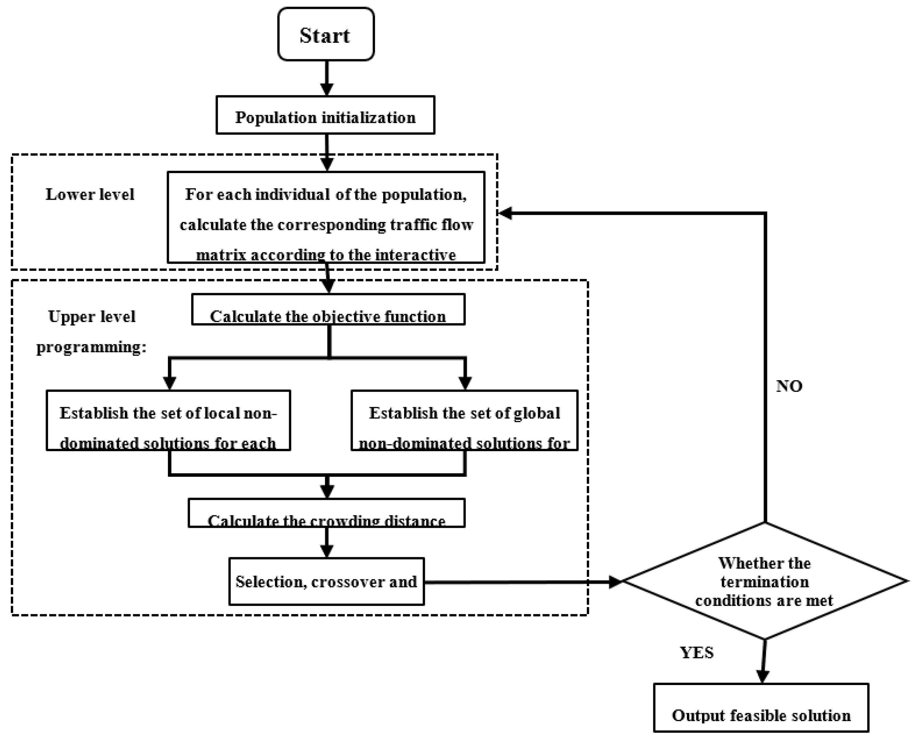
It can be seen from the above model that the multi-objective bi-level programming problem has the characteristics of multivariable and nonlinear; therefore, in this paper, we designed a solution algorithm in which the swarm intelligence multi-objective optimization algorithm is combined with the equalization algorithm of OD matrix. The algorithm steps are as follows:

Step 1: Population initialization. In recent years, swarm intelligence optimization algorithm based on complex network has been proven to be very effective in avoiding local optimum. Therefore, we first establish a network with grid structure for the population and introduce the small world network generation algorithm to depict the connections between individuals in the population, where each individual represents a solution $\left(\mathbf{X},P_r\right)$.

Step 1.1: Set the region $i^{\prime }\in \left[0,n_p\right]$, $j^{\prime }\in \left[0,n_p\right]$ as the complex network generation area; both $i^{\prime }$ and $j^{\prime }$ are integers, and each node $\left(i^{\prime },j^{\prime }\right)$ represents an individual in the population.

Step 1.2: Each individual $\left(i^{\prime },j^{\prime }\right)$ establishes connection with the surrounding eight neighbors to form a cellular network.

Step 1.3: Here, we introduce the method in literature [24]. Let $p_{cut}$ be the rewiring probability of the network, $p_{cut}\in \left[0,1\right]$. We set a random number $p_{rand}\in \left[0,1\right]$ for each node $\left(i^{\prime },j^{\prime }\right)$; if $p_{rand}\le p_{cut}$, cut one of node $\left(i^{\prime },j^{\prime }\right)$’s links randomly, and then establish a new link between node $\left(i^{\prime },j^{\prime }\right)$ and a node that is not in the surrounding eight neighbors of node $\left(i^{\prime },j^{\prime }\right)$. Thus, the new neighborhood is established. In order to make the population space achieve a better balance between complete certainty and complete randomness, we set $p_{cut}=0.5$.

Step 2: The real encoding technique is employed, and the solution corresponding to individual $\left(i^{\prime },j^{\prime }\right)$ is ${\left(\mathbf{X},P_r\right)}_{i^{\prime },j^{\prime }}$, in which the $X_{r,i}$ in $\mathbf{X}$ is encoded with random number between 0 and 1. A random number larger than 0.5 means $X_{r,i}=1$, otherwise $X_{r,i}=0$.

Due to the existence of equilibrium conditions in the group Bush–Mosteller model, given the bus stop schedule plan (represented as the 0–1 matrix $\mathbf{X}$) and the differentiated ticket fares ${\mathbf{P}}_r$($r\in R$), through the continuous iteration of $T_{i,j}^{\kappa ,t}$, $C_{i,j}^{\kappa ,t}$, and $M_{i,j}^t$, the equilibrium traffic flow OD matrix of various travel modes between bus stops can be obtained. The OD matrix equalization algorithm is designed as follows:

Step 2.1: Within a certain distance $d_{i,j}\le d^{\ast }$, there is a competitive relationship between bus and shared bike; for each OD pair in $\mathbf{D}$, given the bus ticket fare $P_r\cdot d_{i,j}$ ($r\in R$), the shared bike management department will set the optimal equilibrium bike sharing fee ${\tilde{P}}_b$ on the basis of generalized Nash equilibrium.

$$\{\begin{array}{l}\{\begin{array}{l}{\tilde{P}}_b^k=\arg \max \left[{\widehat{Q}}_b^k\left({\overline{P}}_r^{k-1}\right)\cdot {\tilde{P}}_b^k\right]\\ {\overline{P}}_r^k=\arg \max \left[{\widehat{Q}}_r^k\left({\tilde{P}}_b^{k-1}\right)\cdot {\overline{P}}_r^k\right]\end{array}\\ {\widehat{Q}}_b^k\left({\overline{P}}_r^{k-1}\right)=Q_b^{k-1}+\frac{\partial Q_b}{\partial {\overline{P}}_r}\left({\overline{P}}_r^k-{\overline{P}}_r^{k-1}\right)+\frac{\partial Q_b}{\partial {\tilde{P}}_b}\left({\tilde{P}}_b^k-{\tilde{P}}_b^{k-1}\right)\\ Q_b^{k-1}=\arg \min \hspace{0.17em}{\displaystyle {\int }_0^{Q_b^{k-1}}G\left({\tilde{P}}_b^{k-1}\right)\mathrm{d}x}\hspace{0.17em}\\ \mathrm{s}.\mathrm{t}.\hspace{0.17em}{\tilde{P}}_b^{\min }\le {\tilde{P}}_b^k\le {\tilde{P}}_b^{\max },r\in R\end{array}$$

(28)

Equation (28) is a generalized Nash equilibrium problem in which $\min \hspace{0.17em}{\int }_0^{Q_b^{k-1}}G\left({\tilde{P}}_b^{k-1}\right)\mathrm{d}x$ represents the estimation of traffic flow by shared bike operators, and it can be calculated on the basis of logit model, where $\frac{\partial Q_b}{\partial {\overline{P}}_r}$ and $\frac{\partial Q_b}{\partial {\tilde{P}}_b}$ represent the derivative relationship between traffic flow and the price of shared bike. Equation (28) can be solved by the method of classical sensitivity analysis, but we will not go into much detail here.

Step 2.2: For the given bus stop schedule plan $\mathbf{X}$, differentiated ticket fares ${\mathbf{P}}_r$, parking fee ${\tilde{P}}_p$, and bike sharing fee ${\tilde{P}}_b$, set the initial value of $C_{i,j}^{r,0}$ and $M_{i,j}^0$ to 0; set the iteration time $t=0$; and calculate the OD flow matrix $Q^{\kappa ,t}$ on the basis of Equations (10)–(14).

Step 2.3: Substitute the $Q^{\kappa ,t}$ into Equation (2) and calculate the traffic flow $f_{i,i+1}^{r+,t+1}$ and $f_{i,i+1}^{r+,t+1}$ of bus lines; then, the value of $C_{i,j}^{r,t+1}$ and $C_{i,j}^{r-,t+1}$ are obtained. Moreover, the number of travelers that choose other travel mode (${\displaystyle \sum _{y\ne x}{\mu }_y}$) is obtained; substitute ${\displaystyle \sum _{y\ne x}{\mu }_y}$ into Equation (4) and the value of $M_{i,j}^{t+1}$ is calculated.

Step 2.4: The generalized travel cost matrix ($\mathbf{G}=\left(\begin{array}{ccc}{G}_{1,1}& \cdots & G_{1,N}\\ ⋮& G_{i,j}& ⋮\\ G_{N,1}& \cdots & G_{N,N}\end{array}\right)$) between bus stops is calculated according to Equation (5).

Step 2.5: Update the OD matrix of traffic flow according to Equations (10)–(14) on the basis of the new $\mathbf{G}$, and the $Q^{\kappa ,t+1}$ is obtained.

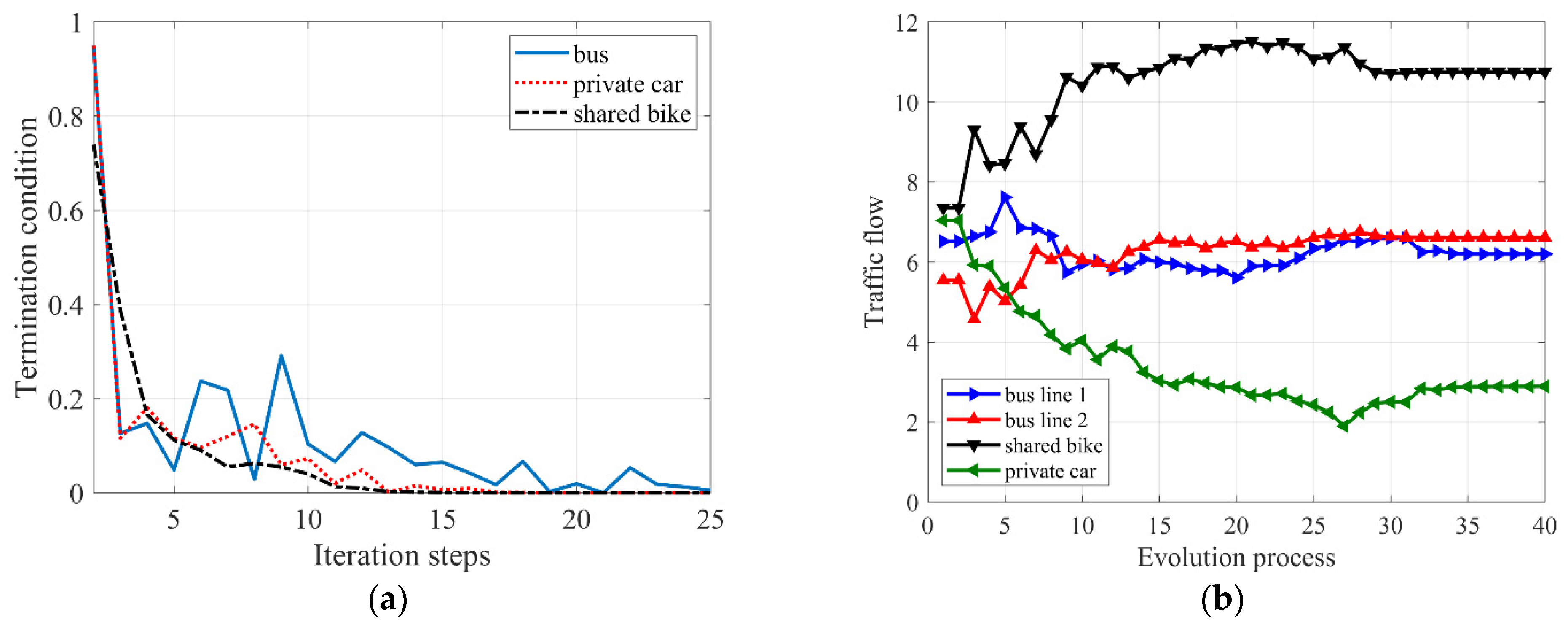
Step 2.6: For all the travel mode $\kappa$, let $\underset{i,j\in V,i\ne j}{\max }\left\{\frac{\left|Q_{i,j}^{\kappa ,t+1}-Q_{i,j}^{\kappa ,t}\right|}{Q_{i,j}^{\kappa ,t}}\le \varsigma \right\}$ represent the termination condition (flow difference between different evolution steps). If this condition is satisfied, the algorithm will stop the iteration; otherwise, return to Step 2.3. Thus, $Q^{\kappa ,t+1}$ is the traffic flow matrix corresponding to the given bus stop schedule plan (the 0–1 matrix $\mathbf{X}$) and the differentiated ticket fares ${\mathbf{P}}_r$($r\in R$). Then, calculate the objective function $F\left(\mathbf{X},P_r\right)={\left[F_1\left(\mathbf{X},P_r\right),F_2\left(\mathbf{X},P_r\right)\right]}^T$ based on $Q^{\kappa ,t+1}$.

Step 3: Establish the set of local non-dominated solutions for each individual in the population. Let $N{D}_{i^{\prime },j^{\prime }}$ denote the non-dominated solutions set of individual $\left(i^{\prime },j^{\prime }\right)$. Add the objective function values (solutions) of individual $\left(i^{\prime },j^{\prime }\right)$’s neighbors $F{\left(\mathbf{X},P_r\right)}_{n{i}^{\prime },n{j}^{\prime }}$ into $N{D}_{i^{\prime },j^{\prime }}$: if the solution in $N{D}_{i^{\prime },j^{\prime }}$ is dominated by the newly added solution ($F{\left(\mathbf{X},P_r\right)}_{n{i}^{\prime },n{j}^{\prime }}\succ N{D}_{i^{\prime },j^{\prime }}\left(k^{\prime }\right)$), then delete the dominated solution in $N{D}_{i^{\prime },j^{\prime }}$; if the newly added solution is not dominated by any solution in $N{D}_{i^{\prime },j^{\prime }}$, add the new solution into $N{D}_{i^{\prime },j^{\prime }}$.

Step 4: Establish the set of global non-dominated solutions for all individuals. Let $N{D}_g$ denote the global non-dominated solutions set, and add the objective function values (solutions) of every node of the population into $N{D}_g$: if the solution in $N{D}_g$ is dominated by the newly added solution ($F{\left(\mathbf{X},P_r\right)}_{i^{\prime },j^{\prime }}\succ N{D}_g\left(k^{\prime }\right)$), then delete the dominated solution in $N{D}_g$; if the newly added solution is not dominated by any solution in $N{D}_g$, add the new solution into $N{D}_g$.

In terms of the constraint condition, we introduce the method of “constraint violation value” to illustrate the constraint violation degree of a solution; the constraint violation value is formulated as

$$CV\left[{\left(\mathbf{X},P_r\right)}_{i^{\prime },j^{\prime }}\right]=\langle {\displaystyle \sum _{i\in V}{\displaystyle \sum _{j\in V}{\displaystyle \sum _{r\in R}{Q}_{i,j}^r\cdot P_r\cdot d_{i,j}}}}\le M\rangle$$

(29)

where $\langle x\rangle$ means if $x\le 0$, then $\langle x\rangle =0$, otherwise $\langle x\rangle =\left|x\right|$. It can be seen that the smaller the value of $CV$, the better the solution is. Therefore, the dominance between two solutions $F{\left(\mathbf{X},P_r\right)}_1$ and $F{\left(\mathbf{X},P_r\right)}_2$ can be redefined as

$F{\left(\mathbf{X},P_r\right)}_1$ dominates $F{\left(\mathbf{X},P_r\right)}_2$ if one of the following conditions is satisfied: (1) $F{\left(\mathbf{X},P_r\right)}_1$ is a feasible solution, but $F{\left(\mathbf{X},P_r\right)}_2$ is non-feasible solution; (2) Both $F{\left(\mathbf{X},P_r\right)}_1$ and $F{\left(\mathbf{X},P_r\right)}_2$ are non-feasible solutions, and $CV\left[{\left(\mathbf{X},P_r\right)}_1\right]<CV\left[{\left(\mathbf{X},P_r\right)}_2\right]$; (3) Both $F{\left(\mathbf{X},P_r\right)}_1$ and $F{\left(\mathbf{X},P_r\right)}_2$ are feasible solutions, and $F{\left(\mathbf{X},P_r\right)}_1$ Pareto dominates $F{\left(\mathbf{X},P_r\right)}_2$.

Step 5: Calculate the crowding distance in $N{D}_{i^{\prime },j^{\prime }}$ and $N{D}_g$. Taking $N{D}_g$ as an example, the solutions in $N{D}_g$ are arranged in descending order from 1 to $N_{k^{\prime }}$ according to the objective function value $F_s{\left(\mathbf{X},P_r\right)}_{k^{\prime }}$$\left(s=1,2,k^{\prime }\in \left[1,N_{k^{\prime }}\right]\right)$, where $N_{k^{\prime }}$ represents the number of solutions. The crowding distance of the $k^{\prime }$th solution of the objective function $s$ is formulated as

$$\{\begin{array}{l}di{s}_{s,k^{\prime }}=F_s{\left(\mathbf{X},P_r\right)}_{k^{\prime }+1}-F_s{\left(\mathbf{X},P_r\right)}_{k^{\prime }-1}\\ di{s}_{s,k^{\prime }}=\infty ,k^{\prime }=1\hspace{0.17em}or\hspace{0.17em}{k}^{\prime }=N_{k^{\prime }}\end{array}$$

(30)

Then, the crowding distance of the $k^{\prime }$th solution is $di{s}_{k^{\prime }}={\displaystyle \sum _{s=1}^{2}di{s}_{s,k^{\prime }}}$.

Step 6: Selection. We introduce the “roulette” method to select the optimal solution in $N{D}_{i^{\prime },j^{\prime }}$ and $N{D}_g$, and thus the probability of individual corresponding to the $k^{\prime }$ solution being selected is $di{s}_{k^{\prime }}/{\displaystyle \sum di{s}_{k^{\prime }}}$; the individual selected in $N{D}_{i^{\prime },j^{\prime }}$ are marked as $\left(i^{″},j^{″}\right)$, and individual selected in $N{D}_g$ are marked as $\left(i^{‴},j^{‴}\right)$.

Step 7: Crossover. Set $\mathbf{Y}=\left(\mathbf{X},P_r\right)$. According to the literature [24], let ${\mathbf{\mu }}_{i^{\prime },j^{\prime }}=\left({\mathbf{Y}}_{i^{″},j^{″}}+{\mathbf{Y}}_{i^{‴},j^{‴}}\right)/2$ and ${\mathbf{\sigma }}_{i^{\prime },j^{\prime }}=\left|{\mathbf{Y}}_{i^{″},j^{″}}-{\mathbf{Y}}_{i^{‴},j^{‴}}\right|$, then the crossover between ${\mathbf{Y}}_{i^{″},j^{″}}$ and ${\mathbf{Y}}_{i^{‴},j^{‴}}$ is formulated as

$${\mathbf{Y}}_{i^{\prime },j^{\prime }}=N\left({\mathbf{\mu }}_{i^{\prime },j^{\prime }},{\mathbf{\sigma }}_{i^{\prime },j^{\prime }}^2\right)$$

(31)

Step 8: Mutation. Let $p_m$ be the probability of chaotic mutation; here, we use the “tent map” to iterate the chaotic sequence for its good ergodicity. The tent map is formulated as ${\rho }_{t+1}=\{\begin{array}{l}2{\rho }_t,{\rho }_t\in \left[0,0.5\right]\\ 2-2{\rho }_t,{\rho }_t\in \left(0.5,1\right]\end{array}$, and the individual is updated according to the probability $p_m$(the value range of ${\mathbf{Y}}_{i^{\prime },j^{\prime }}$ is $\left[{\mathbf{Y}}_{i^{\prime },j^{\prime },\min },{\mathbf{Y}}_{i^{\prime },j^{\prime },\max }\right]$):

$${\mathbf{Y}}_{i^{\prime },j^{\prime }}={\mathbf{Y}}_{i^{\prime },j^{\prime },\min }+{\rho }_t\left({\mathbf{Y}}_{i^{\prime },j^{\prime },\max }-{\mathbf{Y}}_{i^{\prime },j^{\prime },\min }\right)$$

(32)

Step 9: Determining whether the algorithm meets the termination condition (the Pareto front cannot be improved). If so, the algorithm stops, otherwise, return to Step 2.

The flow chart of the solution algorithm is illustrated in Figure 2.

7. Case Study: Optimization of Bus Line and Fares of Fourth Ring Road in Beijing

7.1. Case and Parameter Setting

At present, there are two bus circle lines on the Fourth Ring Road in Beijing (bus no. 400 and bus no. 400 fast; bus no. 400 fast does not stop at every bus stop), and the abovementioned model is introduced to design the feasible differentiated bus lines. In this paper, 12 bus stops of bus no. 400 with large traveler flow on the Fourth Ring Road in Beijing were selected as the object bus stops (see Figure 3; bus stops with very few travelers were not considered). The OD matrix was obtained from the average passenger flow data between bus stops recorded within one month (bus card data). If there was no special explanation later, then we illustrated the parameters of the model and algorithm in

Table 2. Average travel demand among bus stops in a real case.

Travel Demand Dij	1. Wu Ke Song Qiao Nan	2. Si Ji Qing Qiao Nan	3. Zhong Guan Cun Yi Jie	4. Xue Yuan Qiao Dong	5. An Hui Qiao Dong	6. Wang Jing Qiao Dong	7. Hong Ling Jin Qiao Bei	8. Da Jiao Ting Qiao Nan	9. Xiao Hong Men Qiao	10. Huang Tu Gang	11. Yi Hai Hua Yuan	12. Bei Da Di
1. Wu Ke Song Qiao Nan	0	26.45	19.16	18.83	20	5.93	2.68	2.68	2.68	2.68	2.68	2.68
2. Si Ji Qing Qiao Nan	10.54	0	36.44	22.89	27.34	15.33	12.44	11.68	11.54	10.54	11.54	11.74
3. Zhong Guan Cun Yi Jie	5.57	10.2	0	13.31	28.57	17.47	11.07	7.13	8.3477	6.57	5.57	6.57
4. Xue Yuan Qiao Dong	3.77	4.77	4.77	0	52.44	23.8	10.7	5.86	5.53	4.77	4.77	4.97
5. An Hui Qiao Dong	11.14	12.96	11.14	30.68	0	46.34	31.49	17.44	13.76	12.94	12.22	12.64
6. Wang Jing Qiao Dong	2	2	2	3	38.12	0	20.87	11.7	4.67	3.47	4	3.33
7. Hong Ling Jin Qiao Bei	3.39	4.39	3.39	3.39	3.39	4.39	0	9.17	15.25	8.45	10.06	6.39
8. Da Jiao Ting Qiao Nan	4.54	5.54	5.54	5.54	4.54	5.87	6.39	0	12.97	4.54	4.54	5.54
9. Xiao Hong Men Qiao	1.9	1.9	1.9	1.9	1.9	1.9	1.9	1.9	0	11.31	23.8	6.1
10. Huang Tu Gang	6.56	4.21	3.735	3.96	3.36	3.36	3.36	3.36	4.8	0	32.39	18.71
11. Yi Hai Hua Yuan	6.48	4.54	2.49	2.32	2.29	2.18	2.18	2.18	2.18	1.18	0	27.08
12. Bei Da Di	45.23	26.03	22.96	22.64	22.34	22.2	22.7	22.2	22.56	25.49	21.2	0

and

Table 3. Parameter setting.

Symbol	Meaning	Value	Symbol	Meaning	Value
$n_p\times n_p$	population size of the swarm algorithm	25	$d^{\ast }$	critical distance of bicycle riding	5 (km)
$N_{\max }^{line}$	maximum number of bus lines	5	${\varphi }_r$	departure frequency of bus line	5
${\zeta }_{psy},{\zeta }_T,{\zeta }_C,{\zeta }_P,{\zeta }_M$	cost coefficients	0.05	$l$	travelers’ learning intensity	0.9
${\lambda }_m$	social interaction level	1.5	$L$	traveler’s memory length	10
$V^r$	bus capacity	150	$p_c$	traveler’s interaction intensity of risk aversion	0.8
$\left[P_r^{\min },P_r^{\max }\right]$	fare range of bus per kilometer	[0, 0.5]	${\tilde{P}}_p$	parking fee	10
${\psi }_x^t$	travelers’ regret aversion level	[0, 1]	$N_{agent}$	the number of agents in reinforcement learning	100
$p_m$	mutation probability	0.01	$c_r$	average operating cost	10

.

Table 3 illustrates the parameter setting of the model, in which the value of ${\lambda }_m$ and $c_r$ are determined on the basis of the literature [10], the fare range of bus per kilometer and parking fee are determined on the basis of the mean value of real price in Beijing and the value range is appropriately expanded, and the average departure frequency of a bus line is determined by recording the departure frequency at the important bus stop. It is difficult for travelers to remember their travel experience every day in the past, and thus we set the value of $L$ to 10 and set the value of $N_{agent}$ to 100 to ensure that the evolution results of BM model can converge in limited iteration time. By summarizing the relevant literature [25], we found that when the average travel distance is less than 5 km, there will be a demand for shared bike; thus, we set $d^{\ast }=5$.

7.2. Convergence of OD Matrix Equalization Algorithm

Step 2 of the solution algorithm in Section 6 is the OD matrix equalization algorithm; here, we first verified the Theorem 1 by numerical simulation under different bus line planning.

In Figure 4a, the vertical axis represents the mean value of $\frac{\left|Q_{i,j}^{\kappa ,t+1}-Q_{i,j}^{\kappa ,t}\right|}{Q_{i,j}^{\kappa ,t}}$ in all the OD pairs (Table 2); after about 20 steps of iteration, the value tends to 0. Figure 4b–d shows the traffic flow evolution among some typical OD pairs with 2, 3, and 4 bus lines, respectively. It can be seen that the OD matrix equalization algorithm based on multi-agent reinforcement learning and social interaction can make the traffic flow between bus stops converge to a stable state. Theorem 1 is numerically verified under the condition of OD matrix (multi-OD pairs).

7.3. Optimization Results of the Differentiated Bus Lines and Fares

The optimization results of the multi-objective bi-level programming model in this paper can be illustrated by the Pareto front obtained through the above solution algorithm. Moreover, in order to compare the effects of different travel choice models (complete rationality and bounded rationality) on the optimization results, we also introduced the traditional logit model based on regret theory (lower level of (27), $\beta =l$, $\psi =0.5$) to simulate the travel mode choice behavior:

$$\{\begin{array}{l}{\overline{h}}_{i,j}^{\kappa ,t}=G_{i,j}^{\kappa ,t}-\delta \left(\underset{\kappa \in \left\{R,p,b\right\}}{\min }\left\{{G^{\prime }}_{i,j}^{\kappa ,t}\right\}-{G^{\prime }}_{i,j}^{\kappa ,t}\right)\\ Q_{i,j}^{\kappa }=D_{i,j}\cdot \frac{\exp \left(-\beta \cdot {\overline{h}}_{i,j}^{\kappa ,t}\right)}{{\displaystyle \sum _{\kappa \in \left\{R,p,b\right\}}\exp \left(-\beta \cdot {\overline{h}}_{i,j}^{\kappa ,t}\right)}}\end{array}$$

(33)

Figure 5 illustrates the Pareto optimal solutions obtained by the multi-objective bi-level programming based on the two travel choice models (BM reinforcement learning model with interaction and logit model), and

Table 4. Representative Pareto optimal solution based on BM reinforcement learning model.

Scheme 1
Stop Schedule Plans	1. Wu Ke Song Qiao Nan	2. Si Ji Qing Qiao Nan	3. Zhong Guan Cun Yi Jie	4. Xue Yuan Qiao Dong	5. An Hui Qiao Dong	6. Wang Jing Qiao Dong	7. Hong Ling Jin Qiao Bei	8. Da Jiao Ting Qiao Nan	9. Xiao Hong Men Qiao	10. Huang Tu Gang	11. Yi Hai Hua Yuan	12. Bei Da Di	Fare per Kilometer
Bus no. 400	1	1	1	1	1	1	1	1	1	1	1	1	0.0041
Bus line 1	0	0	0	0	0	1	1	1	0	1	1	0	0.0091
Bus line 2	0	0	0	0	0	0	1	1	1	0	1	0	0.1132
Bus line 3	1	0	1	1	1	1	0	0	0	1	1	0	0.3668
Bus line 4	1	1	1	1	1	1	1	1	0	1	1	1	0.3853
Solution B2
Stop Schedule Plans	1. Wu Ke Song Qiao Nan	2. Si Ji Qing Qiao Nan	3. Zhong Guan Cun Yi Jie	4. Xue Yuan Qiao Dong	5. An Hui Qiao Dong	6. Wang Jing Qiao Dong	7. Hong Ling Jin Qiao Bei	8. Da Jiao Ting Qiao Nan	9. Xiao Hong Men Qiao	10. Huang Tu Gang	11. Yi Hai Hua Yuan	12. Bei Da Di	Fare per Kilometer
Bus no. 400	1	1	1	1	1	1	1	1	1	1	1	1	0.4321
Bus line 1	0	0	1	0	1	1	0	0	1	0	1	1	0.2245
Bus line 2	0	1	1	0	0	0	1	1	1	1	1	1	0.2838
Bus line 3	1	1	1	0	1	0	1	1	1	1	1	1	0.3405
Bus line 4	1	1	0	1	0	1	1	1	0	1	0	1	0.2402
Solution B3
Stop Schedule Plans	1. Wu Ke Song Qiao Nan	2. Si Ji Qing Qiao Nan	3. Zhong Guan Cun Yi Jie	4. Xue Yuan Qiao Dong	5. An Hui Qiao Dong	6. Wang Jing Qiao Dong	7. Hong Ling Jin Qiao Bei	8. Da Jiao Ting Qiao Nan	9. Xiao Hong Men Qiao	10. Huang Tu Gang	11. Yi Hai Hua Yuan	12. Bei Da Di	Fare per Kilometer
Bus no. 400	1	1	1	1	1	1	1	1	1	1	1	1	0.4864
Bus line 1	1	1	1	0	1	0	1	0	1	0	1	0	0.4704
Bus line 2	1	1	1	1	0	1	1	1	1	1	1	1	0.0910
Bus line 3	1	1	1	0	1	1	0	0	1	1	1	0	0.3836
Bus line 4	0	1	0	0	0	1	1	0	1	1	1	0	0.4724

and

Table 5. Representative Pareto optimal solution based on logit model.

Solution L1
Stop Schedule Plans	1. Wu Ke Song Qiao Nan	2. Si Ji Qing Qiao Nan	3. Zhong Guan Cun Yi Jie	4. Xue Yuan Qiao Dong	5. An Hui Qiao Dong	6. Wang Jing Qiao Dong	7. Hong Ling Jin Qiao Bei	8. Da Jiao Ting Qiao Nan	9. Xiao Hong Men Qiao	10. Huang Tu Gang	11. Yi Hai Hua Yuan	12. Bei Da Di	Fare per Kilometer
Bus no. 400	1	1	1	1	1	1	1	1	1	1	1	1	0.1954
Bus line 1	1	1	1	1	0	1	0	1	1	0	0	1	0.2473
Bus line 2	0	1	1	0	0	0	1	0	0	1	0	0	0.3761
Bus line 3	1	1	0	0	0	1	0	1	1	0	1	0	0.2140
Bus line 4	1	0	1	1	1	1	0	1	1	1	1	1	0.0372
Solution L2
Stop Schedule Plans	1. Wu Ke Song Qiao Nan	2. Si Ji Qing Qiao Nan	3. Zhong Guan Cun Yi Jie	4. Xue Yuan Qiao Dong	5. An Hui Qiao Dong	6. Wang Jing Qiao Dong	7. Hong Ling Jin Qiao Bei	8. Da Jiao Ting Qiao Nan	9. Xiao Hong Men Qiao	10. Huang Tu Gang	11. Yi Hai Hua Yuan	12. Bei Da Di	Fare per Kilometer
Bus no. 400	1	1	1	1	1	1	1	1	1	1	1	1	0.3338
Bus line 1	0	0	0	1	0	1	0	0	1	1	1	1	0.1492
Bus line 2	0	1	1	1	0	1	1	1	1	1	0	1	0.0632
Bus line 3	0	0	0	0	0	0	1	1	1	0	1	1	0.3072
Bus line 4	1	0	1	0	0	1	0	0	0	1	1	1	0.3573
Solution L3
Stop Schedule Plans	1. Wu Ke Song Qiao Nan	2. Si Ji Qing Qiao Nan	3. Zhong Guan Cun Yi Jie	4. Xue Yuan Qiao Dong	5. An Hui Qiao Dong	6. Wang Jing Qiao Dong	7. Hong Ling Jin Qiao Bei	8. Da Jiao Ting Qiao Nan	9. Xiao Hong Men Qiao	10. Huang Tu Gang	11. Yi Hai Hua Yuan	12. Bei Da Di	Fare per Kilometer
Bus no. 400	1	1	1	1	1	1	1	1	1	1	1	1	0.1500
Bus line 1	0	1	1	0	0	1	0	0	0	1	0	1	0.4658
Bus line 2	0	0	1	0	0	0	0	1	0	0	0	0	0.5621
Bus line 3	0	1	1	0	0	1	1	0	1	1	0	0	0.4197
Bus line 4	0	0	0	0	0	0	0	0	1	0	1	0	0.2452

show the representative Pareto optimal solution based on these two models. It can be seen from Figure 5 that, compared with the traditional logit model with complete rationality, the multi-objective bi-level programming based on BM reinforcement learning model obtained higher travelers’ utility but lower profit, which indicates that the increase of travelers’ learning behavior under the assumption of regret theory improves the effectiveness of group decision making and then reduces the profit of buses. It can also be seen from Table 4 and Table 5 that different travel choice models have significantly changed the optimization results of bus lines and the differentiated fares. Moreover, except for the bus lines that stop at every bus stop, it can be seen from the profit-oriented optimal solutions (solution B3) that the lower the number of bus stops, the higher the ticket fare.

It can be seen from

Table 6. Calculation results of the model.

	BM Reinforcement Learning Model			Logit Model
Pareto Optimal Solution	B1	B2	B3	L1	L2	L3
Generalized travel cost	2.8443	3.9530	4.2712	3.7683	4.5115	5.5936
Average operating profit of buses	−142.8101	−127.2018	−103.8919	−161.8960	−121.2167	−90.0820
$\mathrm{Maximum} \sec \mathrm{tion} \mathrm{flow} (\max \left\{f_{i,i+1}^{r+}+f_{i,i+1}^{r-}\right\}\left(r\in R,i\in V\right)$) of the optimal bus lines	110.8276	80.0160	68.3004	69.3548	92.4435	95.4080
$\mathrm{Maximum} \sec \mathrm{tion} \mathrm{flow} (\max \left\{f_{i,i+1}^{r+}+f_{i,i+1}^{r-}\right\}\left(r\in R,i\in V\right)$) of the optimal bus lines based on real ticket fare	79.1855	84.3061	75.3261	69.5392	92.9450	92.6598

that the continuous evolution of travelers’ regret aversion level in BM reinforcement learning model effectively reduces the generalized travel cost (lower than logit model); therefore, the profit of the BM model is also lower than logit model. Moreover, on the basis of the optimized bus lines, compared with the ticket fare under real case (bus no. 400: RMB 2 within 10 km, RMB 1 for every additional 5 km), the differentiated fares effectively reduce the maximum section flow of bus lines, which means that the balance of passenger flow distribution in the bus network has been improved.

7.4. Effect of Important Parameters on Optimization Results

(1)

Maximum number of bus lines

Change the maximum number of bus lines $N_{\max }^{line}$ and investigate the corresponding changes of the optimal solution.

It can be seen from Figure 6 that with the decrease of $N_{\max }^{line}$, the traveler utility decreases, and the operating profit of buses increases. Furthermore, in reality, there are two bus circle lines on the Fourth Ring Road in Beijing (bus no. 400 and bus no. 400 fast); under the condition of $N_{\max }^{line}=2$, a comparison is made between the corresponding Pareto optimal solution and the bus lines and ticket fares under real case (

Table 7. The comparison between Pareto optimal solution and the real case.

Pareto Optimal Solutions and the Real Case	$\mathit{B}{1}^{\prime }$	$\mathit{B}{2}^{\prime }$	$\mathit{B}{3}^{\prime }$
$\mathrm{Maximum} \sec \mathrm{tion} \mathrm{flow} (\max \left\{f_{i,i+1}^{r+}+f_{i,i+1}^{r-}\right\}\left(r\in R,i\in V\right)$) of the optimal bus lines and differentiated fares	140.1102	89.9407	81.2725
$\mathrm{Maximum} \sec \mathrm{tion} \mathrm{flow} (\max \left\{f_{i,i+1}^{r+}+f_{i,i+1}^{r-}\right\}\left(r\in R,i\in V\right)$) of bus lines under real case (bus no. 400 and bus no. 400 fast in Beijing)	101.3021	96.2163	87.2309
Average operating profit of the optimal bus lines and differentiated fares	−75.3130	−56.5348	−37.3504
Average operating profit of bus lines under real case (bus no. 400 and bus no. 400 fast in Beijing)	−63.0251
Generalized travel cost of the optimal bus lines and differentiated fares	0.4730	0.6485	0.9972
Generalized travel cost of bus lines under real case (bus no. 400 and bus no. 400 fast in Beijing)	0.7104

). Table 7 shows that compared with the bus lines and fares under real case (bus no. 400 and bus no. 400 fast), the multi-objective bi-level programming proposed in this paper can generate the solution to reduce the maximum section flow, increase the profit, and reduce the generalized travel cost, thus reducing congestion.

(2)

Traveler’s learning behavior

On the basis of the optimal bus lines and differentiated fares obtained from the multi-objective bi-level programming, we analyzed the impact of travelers’ behavior on the objective function through numerical simulation.

Figure 7 illustrates the effect of traveler’s learning behavior (travelers’ learning intensity $l$ and traveler’s interaction intensity of risk aversion $p_c$) on generalized travel cost, wherein it can be seen that the generalized travel cost corresponding to the representative Pareto optimal solution decreases with the increase of $l$ and $p_c$. This result indicates that travelers’ reinforcement learning and information exchanging on risk aversion level in the multi-objective bi-level programming are effective; therefore, increasing the dissemination of travel cost information and risk attitude among travelers can effectively reduce travel costs.

7.5. Equilibrium Analysis of Ring Road Bus Line Planning

In reality, the management department of buses is not always able to accurately perceive the complexity of travelers’ decisions; therefore, the management department of buses often predicts group behavior on the basis of general equilibrium theory. Moreover, when taking the social interaction into consideration, we find that the equilibrium condition of travelers from the perspective of bus management department can be formulated as [10]

$$E\left({\xi }_x\right)=\tanh \left\{\beta \left[-{\overline{G^{\prime }}}_{i,j}^{\kappa }+{\lambda }_m\cdot \frac{{\displaystyle \sum _{y\ne x}E\left({\xi }_y\right)}}{{\overline{D}}_{i,j}-1}\right]\right\}$$

(34)

Furthermore, the social equilibrium equation of all travelers among the bus lines can be formulated as

$${\mu }^{\ast }=\tanh \left[\beta \left({\lambda }_m{\mu }^{\ast }-{\overline{G^{\prime }}}_{i,j}^{\kappa }\right)\right]$$

(35)

Here, ${\mu }^{\ast }$ represents the average choice proportion of a travel mode when travelers’ behavior is in equilibrium; therefore, the adjustment of bus lines and travelers’ group behavior can change the social equilibrium. On the basis of the representative Pareto optimal solution, we analyzed the proportion of travel mode choice according to Equation (34) and investigated the impact of optimal bus lines and differentiated fares on the equilibrium.

Figure 8a shows the relationship between subjective expectation curves (based on Equation (34)) of different bus line schemes (Pareto optimal solutions and the bus lines and ticket fares under real case, $N_{\max }^{line}=2$) and travelers’ group selection equilibrium under the multi-agent BM reinforcement learning model. It can be seen that, when ${\lambda }_m=1.5$, neither Pareto optimal solution nor bus lines and ticket fares under real case can make travelers’ subjective expectation and actual decision reach equilibrium; however, compared with the bus lines and ticket fares under real case, the model proposed in this paper produces Pareto optimal solutions that make the subjective expectation curve closer to equilibrium (B1 and B2). Moreover, it can be seen from Figure 8b that, when ${\lambda }_m=2.3$, the Pareto optimal solution B2 reaches unique equilibrium; in this equilibrium state, the proportion of travelers who choose bus is greater than 0.5, and the Pareto optimal solution B1 produces two equilibrium points, namely, advantage equilibrium point (the proportion of travelers who choose bus is greater than 0.5) and disadvantage equilibrium point (the proportion of travelers who choose bus is less than 0.5). Therefore, Figure 8a,b shows that the complexity of travelers’ group behavior will significantly shift the social equilibrium equation, and the increase of social interaction intensity makes the subjective expectation curve move to the upper left. For the management department of buses, different bus line and fare plans (from B1 to B3) will also significantly shift the social equilibrium equation, and thus the management department of buses can appropriately increase the dissemination of accurate travel cost information among travelers to promote the formation of equilibrium.

8. Conclusions

In this paper, a multi-objective bi-level programming model of bus lines and differentiated ticket fares for the urban ring road was proposed. The operating profit and travelers’ utility are taken as objective functions. In the new model we have proposed, travelers’ reinforcement learning behavior and social interaction for higher utility based on regret theory is introduced. Through the numerical analysis based on real bus lines (the bus circle lines on the Fourth Ring Road in Beijing), we made the following conclusions: (1) Travel choice models with different degrees of rationality have significantly changed the optimization results of bus lines and the differentiated fares. (2) Compared with the ticket fare under real case, the differentiated fares effectively reduce the maximum section flow of bus lines. (3) Compared with the bus lines and fares under real case, the multi-objective bi-level programming in this paper can generate the solution to reduce the maximum section flow, increase the profit, and reduce the generalized travel cost. (4) In order to encourage travelers to choose buses, the management department of buses can appropriately increase the dissemination of accurate travel cost information among travelers to promote the formation of advantage equilibrium and to reduce travelers’ travel costs. Moreover, travelers should also increase the intensity of learning and the social interaction of risk aversion level to reduce their generalized travel costs.

In addition, this paper shows that, compared with the logit model with complete information and complete rationality, under the condition of multi-objective optimization, the evolutionary learning behavior of travelers can reduce the operating profit of transportation system. Therefore, it can be seen that, whether under the condition of complete rationality or under the condition of complex cluster behavior, the more accurate travelers master the utility information, the higher the travel utility, and the lower the profit of the transportation system.