Extended Graph of the Fuzzy Topographic Topological Mapping Model

Abstract

Fuzzy topological topographic mapping ($FTTM$) is a mathematical model which consists of a set of homeomorphic topological spaces designed to solve the neuro magnetic inverse problem. A sequence of FTTM, $FTT{M}_n$, is an extension of FTTM that is arranged in a symmetrical form. The special characteristic of $FTTM$, namely the homeomorphisms between its components, allows the generation of new $FTTM$. The generated $FTTM$s can be represented as pseudo graphs. A graph of pseudo degree zero is a special type of graph where each of the $FTTM$ components differs from the one adjacent to it. Previous researchers have investigated and conjectured the number of generated $FTTM$ pseudo degree zero with respect to n number of components and k number of versions. In this paper, the conjecture is proven analytically for the first time using a newly developed grid-based method. Some definitions and properties of the novel grid-based method are introduced and developed along the way. The developed definitions and properties of the method are then assembled to prove the conjecture. The grid-based technique is simple yet offers some visualization features of the conjecture.

1. Introduction

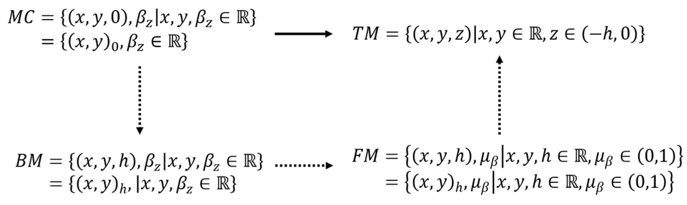
Fuzzy topographic topological mapping (FTTM) [1] was introduced to solve the neuro magnetic inverse problem, particularly with regards to the sources of electroencephalography (EEG) signals recorded from epileptic patients. Originally, the model was a 4-tuple of topological spaces and mappings. The topological spaces are the magnetic plane (MC), base magnetic plane (BM), fuzzy magnetic field (FM) and topographic magnetic field (TM). The third component of FTTM, FM, is a set of three tuples with the membership function of its potential reading obtained from a recorded EEG. FTTM is defined formally as follows (see Figure 1).

Figure 1. The FTTM.

Definition 1.

Ref. [1] Let$FTT{M}_i=\left(M{C}_i,B{M}_i,F{M}_i,T{M}_i\right)$such that$M{C}_i,B{M}_i,F{M}_i,T{M}_i$are topological spaces with$M{C}_i\cong B{M}_i\cong F{M}_i\cong T{M}_i$. Set of$FTT{M}_i$is denoted by$FTTM=\left\{FTT{M}_i:i=1,2,3,\dots ,n\right\}$. Sequence of$nFTT{M}_i$of FTTM is$FTT{M}_1,FTT{M}_2,FTT{M}_3,$$FTT{M}_4,\dots ,FTT{M}_n$such that$M{C}_i\cong M{C}_{i+1},B{M}_i\cong B{M}_{i+1},F{M}_i\cong F{M}_{i+1}$and$T{M}_i\cong T{M}_{i+1}$.

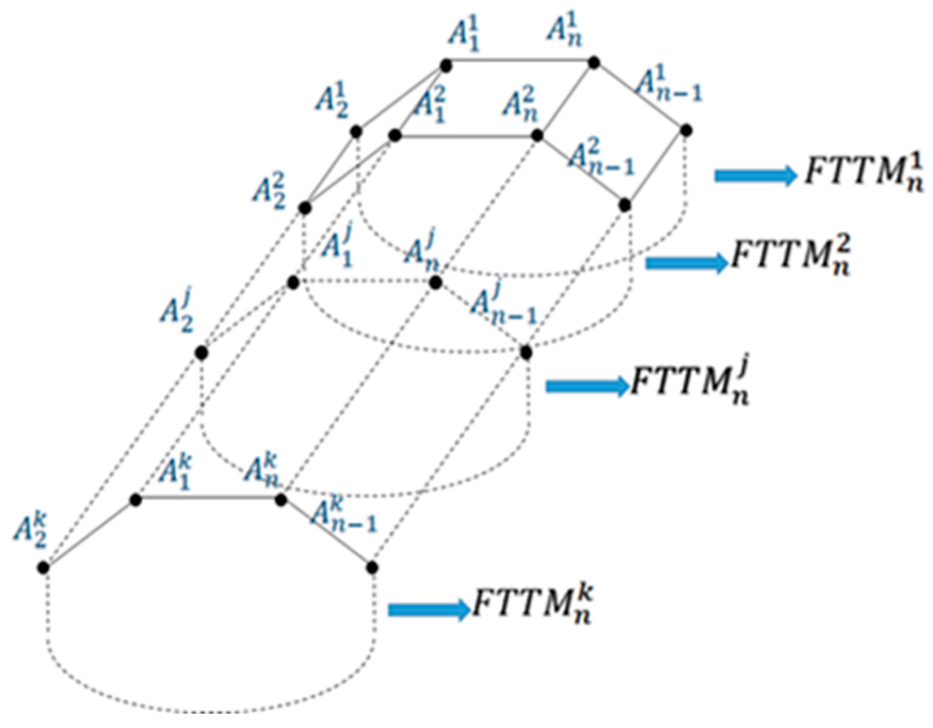
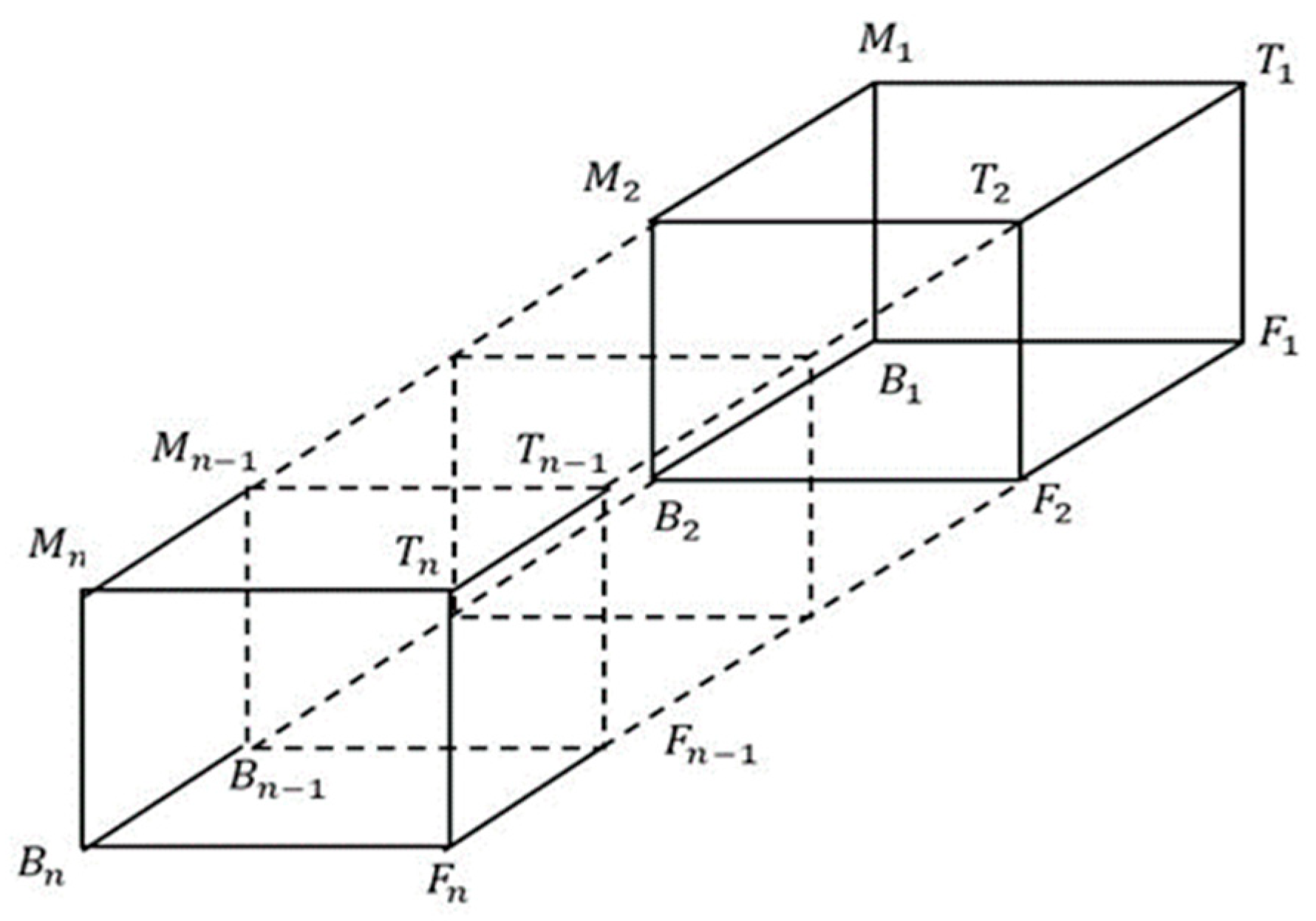
Furthermore, a sequence of FTTM, $FTT{M}_n$, is an extension of FTTM and illustrated in Figure 2. It is arranged in a symmetrical form, since the model can accommodate magnetoencephalography (MEG) signals as well as image data due to its homeomorphism.

Figure 2. The sequence of $FTT{M}_n$.

2. Generalized FTTM

Generally, the FTTM structure can also be expanded for any n number of components.

Definition 2.

Ref. [2] A$FTTM$is defined as

$$FTT{M}_n=\left\{\left\{A_1, A_2, \dots , A_n\right\} : A_1\cong A_2\cong \dots \cong A_n\right\}$$

(1)

such that$A_1, A_2, \dots , A_n$are the components of$FTT{M}_n$

The same generalization can be applied to any k number of $FTTM$ versions as well, denoted as $FTT{M}_n^k$. Without the loss of generality, the collection of the $k$ version of $FTTM, \mathrm{in} \mathrm{short} FTT{M}_n^k,$ is now simply called as a sequence of $FTTM$ unless otherwise stated.

Definition 3.

Ref. [2] A sequence of$k$versions of$FTT{M}_n$denoted by$\ast FTT{M}_n^k$such that

$$\ast FTT{M}_n^k=\left\{FTT{M}_n^1 ,FTT{M}_n^2, \dots , FTT{M}_n^k\right\}$$

(2)

where $FTT{M}_n^1$ is the first version of $FTT{M}_n$, the $FTT{M}_n^2$ is the second version of $FTT{M}_n$ and so forth.

Obviously, a new $FTTM$ can be generated from a combination of components from different versions of $FTTM$ due to their homeomorphisms.

Definition 4.

Ref. [2] A new$FTTM$generated from$\ast FTT{M}_n^k$is defined as

$$F=\left\{A_1^{m_1} ,A_2^{m_2} , . . . , A_n^{m_n}\right\}\in FTTM$$

(3)

where$0 \le m_1, m_2, . . . , m_n \le k$and$m_i\ne m_j$for at least one$i, j$.

A set of elements generated by $\ast FTT{M}_n^k$ is denoted by $G\left(\ast FTT{M}_n^k\right)$. Mukaram et al. [2] showed that the number of $FTTM$can be determined from $\ast FTT{M}_4^k$ using the geometrical features of its graph representation.

Theorem 1.

Ref. [2] The number of generated$FTTM$that can be created from$\ast FTT{M}_4^k$is

$$\left|G\left(\ast FTT{M}_4^k\right)\right|=k^4-k.$$

(4)

Theorem 1 is then extended to include $n$ number of $FTTM$components.

Theorem 2.

Ref. [2] The number of generated FTTM that can be created from$\ast FTT{M}_n^k$is

$$\left|G\left(\ast FTT{M}_n^k\right)\right|=k^n-k.$$

(5)

The following example is presented to illustrate Theorem 2.

Example 1.

Consider$\ast FTT{M}_3^2$, with$FTT{M}_3^1=\left\{A_1^1,A_2^1, A_3^1\right\}$and$FTT{M}_3^2=\left\{A_1^2,A_2^2, A_3^2\right\}$, then$G\left(\ast FTT{M}_3^2\right)=\left\{\left\{A_1^1,A_2^2, A_3^1\right\}, \left\{A_1^1, A_2^1,A_3^2\right\},\left\{A_1^2,A_2^1,A_3^1\right\},\left\{A_1^2,A_2^2,A_3^1\right\}, \left\{A_1^2,A_2^1,A_3^2\right\}, \left\{A_1^1,A_2^2,A_3^2\right\}\right\}$that is$\left|G\left(\ast FTT{M}_3^2\right)\right|=2^3–2=6$as given by Theorem 2.

3. Extended Generalization of FTTM

There are many studies on ordinary and fuzzy hypergraphs available in the literature such as [3,4]. However, $\ast FTT{M}_n^k$ is an extended generalization of FTTM that is represented by a graph of a sequence of $k$ number of polygons with $n$ sides or vertices. The polygon is arranged from back to front where the first polygon represents $FTT{M}_n^1$, the second polygon represents $FTT{M}_n^2$ and so forth. An edge is added to connect $FTT{M}_n^1$ to the $FTT{M}_n^2$ component wisely. A similar approach is taken for $FTT{M}_n^2$, $FTT{M}_n^3$ and the rest (Figure 3).

Figure 3. Graph of $\ast FTT{M}_n^k$.

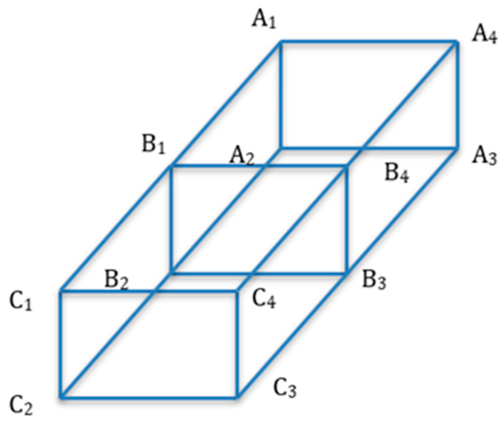
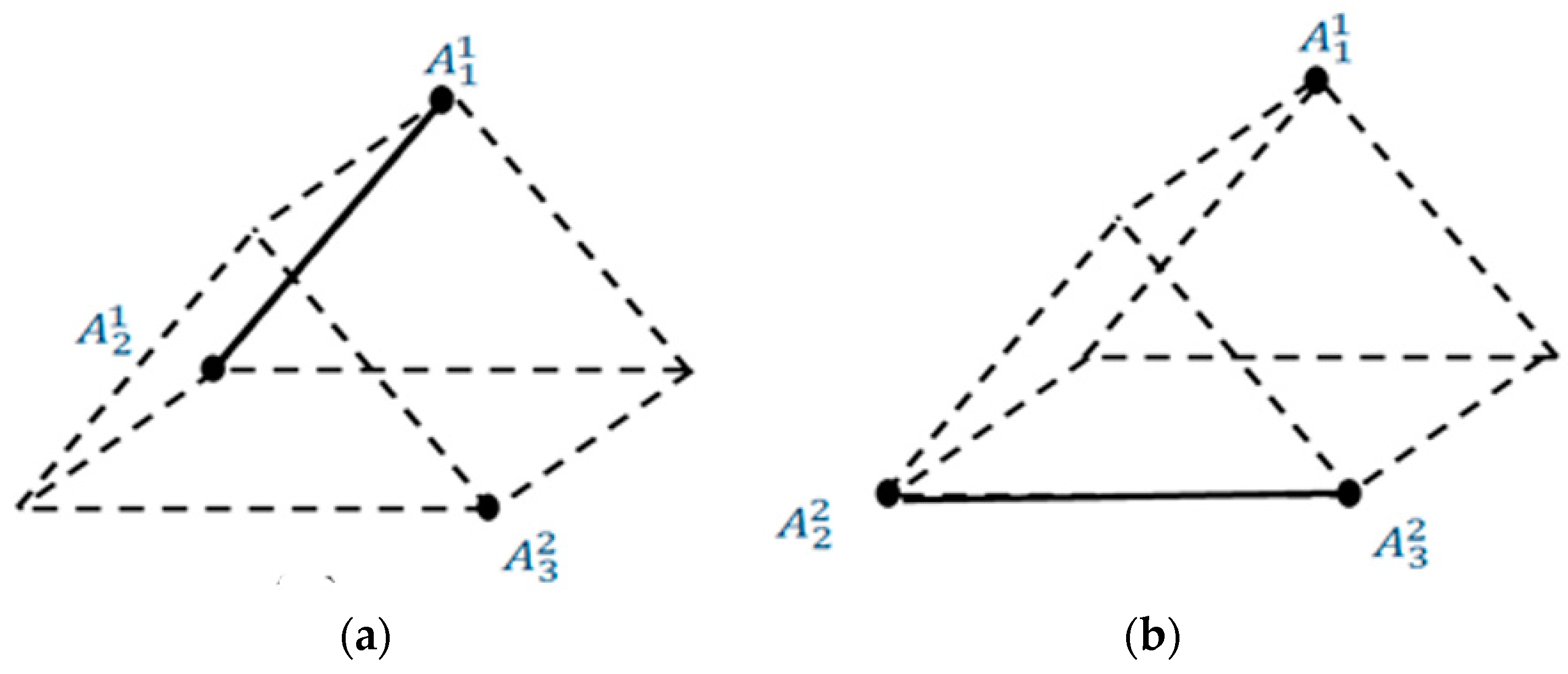
When a new $FTTM$ is obtained from $\ast FTT{M}_n^k$, it is then called a pseudo-graph of the generated $FTTM$ and plotted on the skeleton of $\ast FTT{M}_n^k$. A generated element of a pseudo-graph consists of vertices that signify the generated $FTTM$ and edges which connect the incidence components. Two samples of pseudo-graphs are illustrated in Figure 4.

Figure 4. Pseudo graph: (a) $\left\{A_1^1,A_2^1,A_3^2\right\}$; (b) $\left\{A_1^1,A_2^2,A_3^2\right\}$ of $\ast FTT{M}_3^2$.

Another concept related closely to the pseudo-graph is the pseudo degree. It is defined as the sum of the pseudo degree from each component of the $FTTM$. The pseudo degree of a component is the number of other components that are adjacent to that particular component.

Definition 5.

Ref. [2] The$de{g}_p :FTTM\to Z$defines the pseudo degree of the$FTTM$component. It maps a component of$F\in G\left(\ast FTT{M}_n^k\right)$to an integer

$${\mathit{deg}}_p\left(A_j^{m_j}\right)=\{\begin{array}{c}0; m_{j-1}\ne m_j\ne m_{j+1} \\ 1; m_{j-1}=m_j or m_j=m_{j+1}, \\ 2; m_{j-1}=m_j=m_{j+1}\end{array}$$

(6)

for$A_j^{m_j}\in FTTM$.

Definition 6.

Ref. [2] The$de{g}_{p}G :G\left(\ast FTT{M}_n^k\right)\to Z$defines the pseudo degree of the$FTTM$graph. Let$F \in FTTM$

$$de{g}_{p}G\left(F\right)={{\displaystyle \sum }}_{i=1}^n{\mathit{deg}}_p{A}_i^{m_i}$$

(7)

where$F=\left\{A_1^{m_1} ,A_2^{m_2} , . . . , A_n^{m_n}\right\}\in G\left(\ast FTT{M}_n^k\right)$.

Definition 7.

Ref. [2] The set of elements generated by$\ast FTT{M}_n^k$that have pseudo degree zero is

$$G_0\left(\ast FTT{M}_n^k \right)=\left\{F\in G\left(\ast FTT{M}_n^k\right)|de{g}_{p}G\left(F\right)=0 \right\}$$

(8)

From now on,

• $G_0\left(\ast FTT{M}_n^k \right)$ is simply denoted by $G_0\left(FTT{M}_n^k \right)$.
• $\#G_0\left(FTT{M}_n^k \right)$ denotes the cardinality of the set $G_0\left(FTT{M}_n^k \right)$.

Example 2.

(See Figure 5).

$$\begin{array}{ccc}\hfill FTT{M}_4^3& =& \left\{\left(A_1,A_2,A_3,A_4\right), \left(B_1,B_2,B_3,B_4\right), \left(C_1,C_2,C_3,C_4\right)\right\}\hfill \\ \hfill G_0\left(FTT{M}_4^3\right)& =& \{\left(A_1,B_2,A_3,C_4\right), \left(A_1,B_2,C_3,B_4\right), \left(A_1,C_2,A_3,B_4\right), \left(A_1,C_2,B_3,C_4\right), \hfill \\ & & \left(B_1,A_2,B_3,C_4\right),\left(B_1,A_2,C_3,A_4\right), \left(B_1,C_2,B_3,A_4\right), \left(B_1,C_2,A_3,C_4\right),\hfill \\ & & \left(C_1,B_2,C_3,A_4\right), \left(C_1,B_2,A_3,B_4\right), \left(C_1,A_2,C_3,B_4\right), \left(C_1,A_2,B_3,A_4\right)\}\hfill \\ \hfill G_0\left(FTT{M}_4^3\right)& =& 12.\hfill \end{array}$$

(9)

Figure 5. $FTT{M}_4^3$.

Previously, Elsafi proposed a conjecture in [5] related to the graph of pseudo degree.

Conjecture 1.

Ref. [5]

$$\left|G_0^3\left(FTT{M}_n^3\right)\right|=\{\begin{array}{l}4\left|G_0^3\left(FTT{M}_{n-2}^3\right)\right|+12 , when n is even \\ 4\left|G^3{ }_0\left(FTT{M}_{n-2}^3\right)\right|+6, when n is odd\end{array}$$

(10)

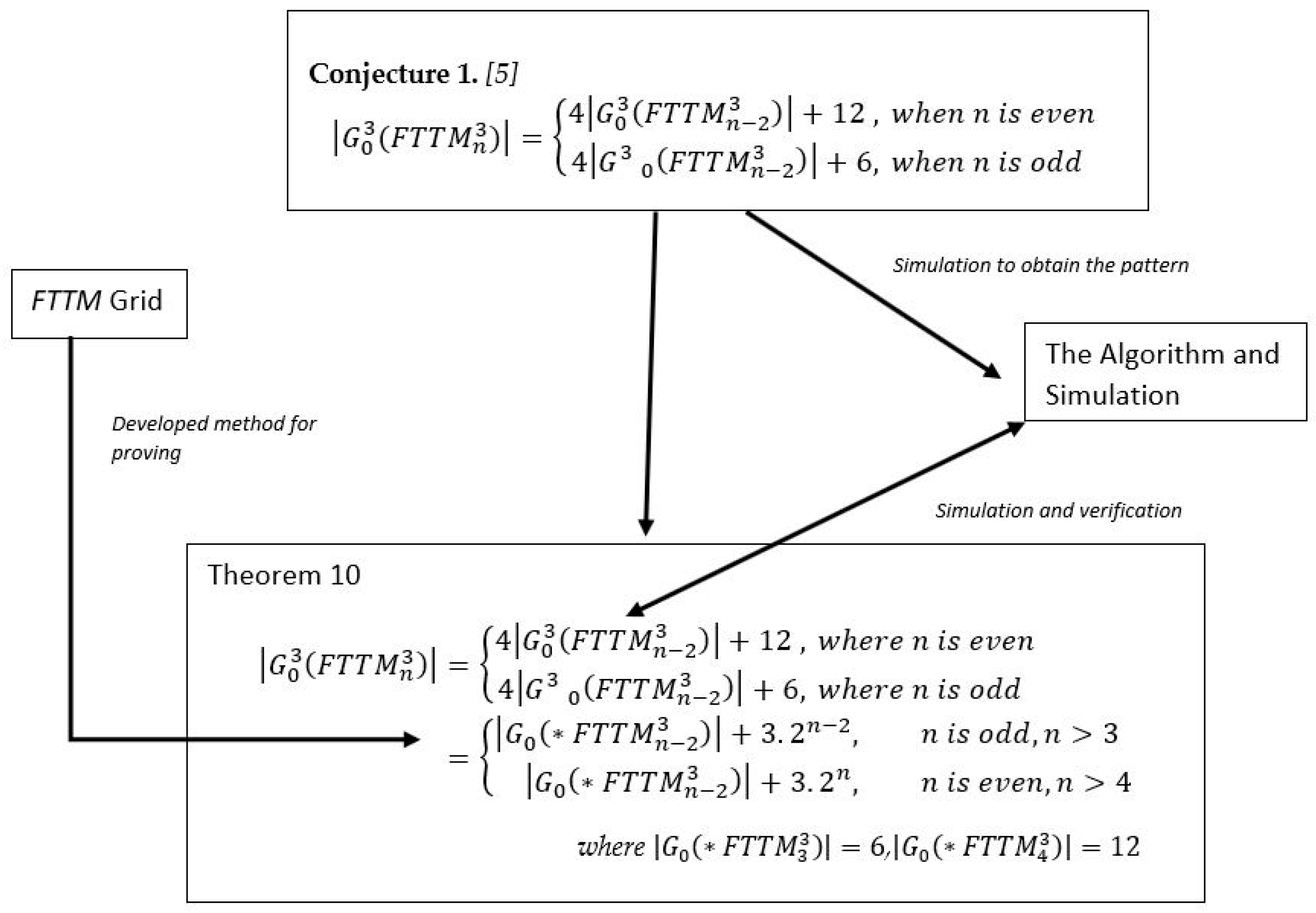
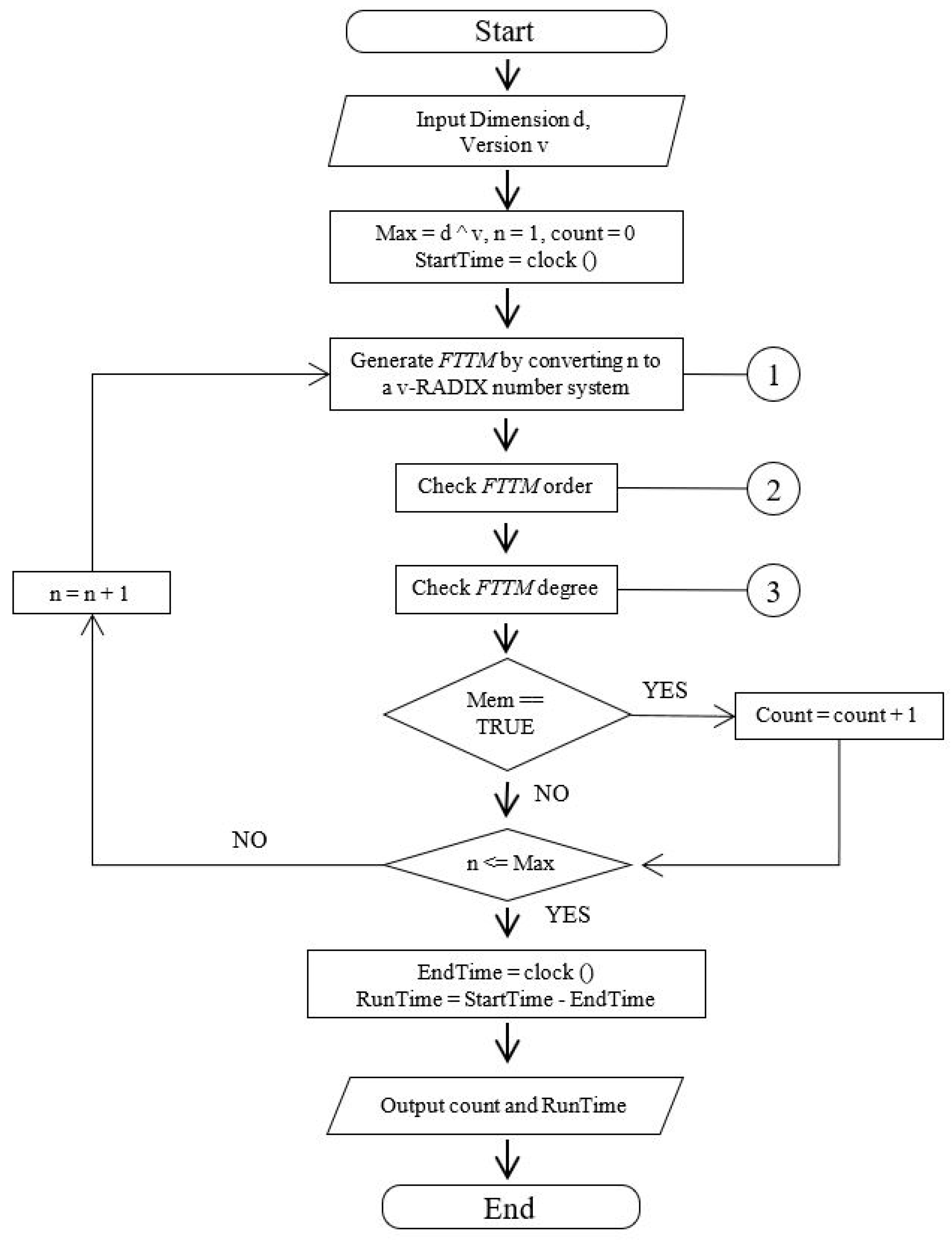
In order to observe some patterns that may appear from the proposed conjecture, Mukaram et al. [2] have developed an algorithm to compute $\left| G_0\left(FTT{M}_n^3 \right)\right|$ in order to prove the conjecture analytically. A flowchart on $\left|G_0\left(\ast FTT{M}_3^n\right)\right|$ is sampled in Figure 6.

Figure 6. Flowchart for determining $\left|G_0\left(\ast FTT{M}_3^n\right)\right|$.

The researchers generated all $FTTM$ combinations for $3\le k\le 4$, $4\le n \le 15$ and were able to isolate graphs with pseudo degree zero, which are listed below (Table 1).

Table 1. $\left| G_0\left(FTT{M}_n^k \right)\right|$ for $4\le n \le 15$ and $k=3,4$.

n	$\left| {\mathit{G}}_0\left(\mathit{F}\mathit{T}\mathit{T}{\mathit{M}}_{\mathit{n}}^3 \right)\right|$	$\left| {\mathit{G}}_0\left(\mathit{F}\mathit{T}\mathit{T}{\mathit{M}}_{\mathit{n}}^4 \right)\right|$
4	12	24
5	30	120
6	60	480
7	126	1680
8	252	5544
9	510	17,640
10	1020	54,960
11	2046	168,960
12	4092	515,064
13	8190	1,561,560
14	16,380	4,717,440
15	32,766	14,217,840

The researchers then simulated $\left| G_0\left(FTT{M}_n^k \right)\right|$ for some values of k as well [2]. The number of graphs of pseudo degree zero for $2\le k\le 8$and $2 \le n \le 10$ are listed in Table 2.

Table 2. $\left|{ G}_0\left(FTT{M}_n^k \right)\right|$ for $2\le k\le 8$and $2 \le n \le 10$.

k/n	2	3	4	5	6	7	8	9	10
2	2	0	2	0	2	0	2	0	2
3	0	6	12	30	60	126	252	510	1020
4	0	0	24	120	480	1680	5544	17,640	54,960
5	0	0	0	120	1080	6720	35,280	168,840	763,560
6	0	0	0	0	720	10,080	90,720	665,280	4,339,440
7	0	0	0	0	0	5040	100,800	1,239,840	12,096,000
8	0	0	0	0	0	0	40,320	1,088,640	17,539,200

4. Grid of FTTM

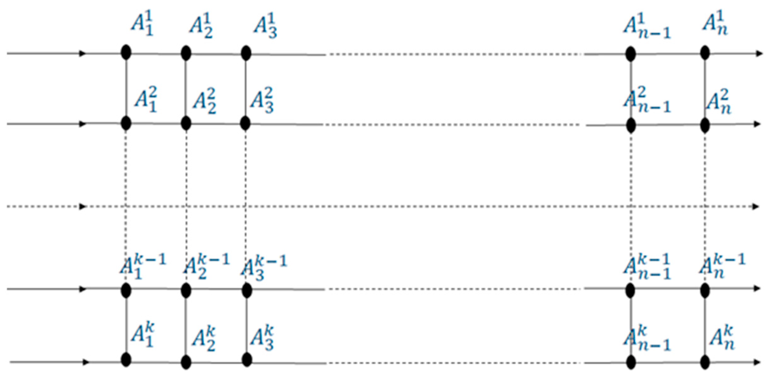
An alternative presentation of a sequence of $FTTM$, called an FTTM grid, is briefly overviewed. It provides a different perspective of the structure of $\mathit{FTTM}$. Instead of a polygon representation for each version of $FTTM$, a straight line is now used. The components of $FTT{M}_n$ are arranged on a horizontal line of vertices and the lines represent the homeomorphisms between the components of $FTT{M}_n$. The only exception is the homeomorphism between the first and last components of $FTT{M}_n, A_1$ and $A_n$, respectively. Two open segments on the left of $A_1$ and on the right of $A_n$ are used to represent the homeomorphism between them. A vertical line is added to represent a homeomorphism between two components of different versions; hence, a grid is created (see Figure 7).

Figure 7. A graph representation of $\ast FTT{M}_n^k$ as a grid.

There are four advantages when FTTM is represented as a grid instead of a sequence of polygon.

• It is represented in two dimensions; therefore, it reduces the complexity of the structure.
• The process of adding a new component is easier than in a sequence of polygon.
• It can take any number of components by adding the number of vertices at the end of the grid.
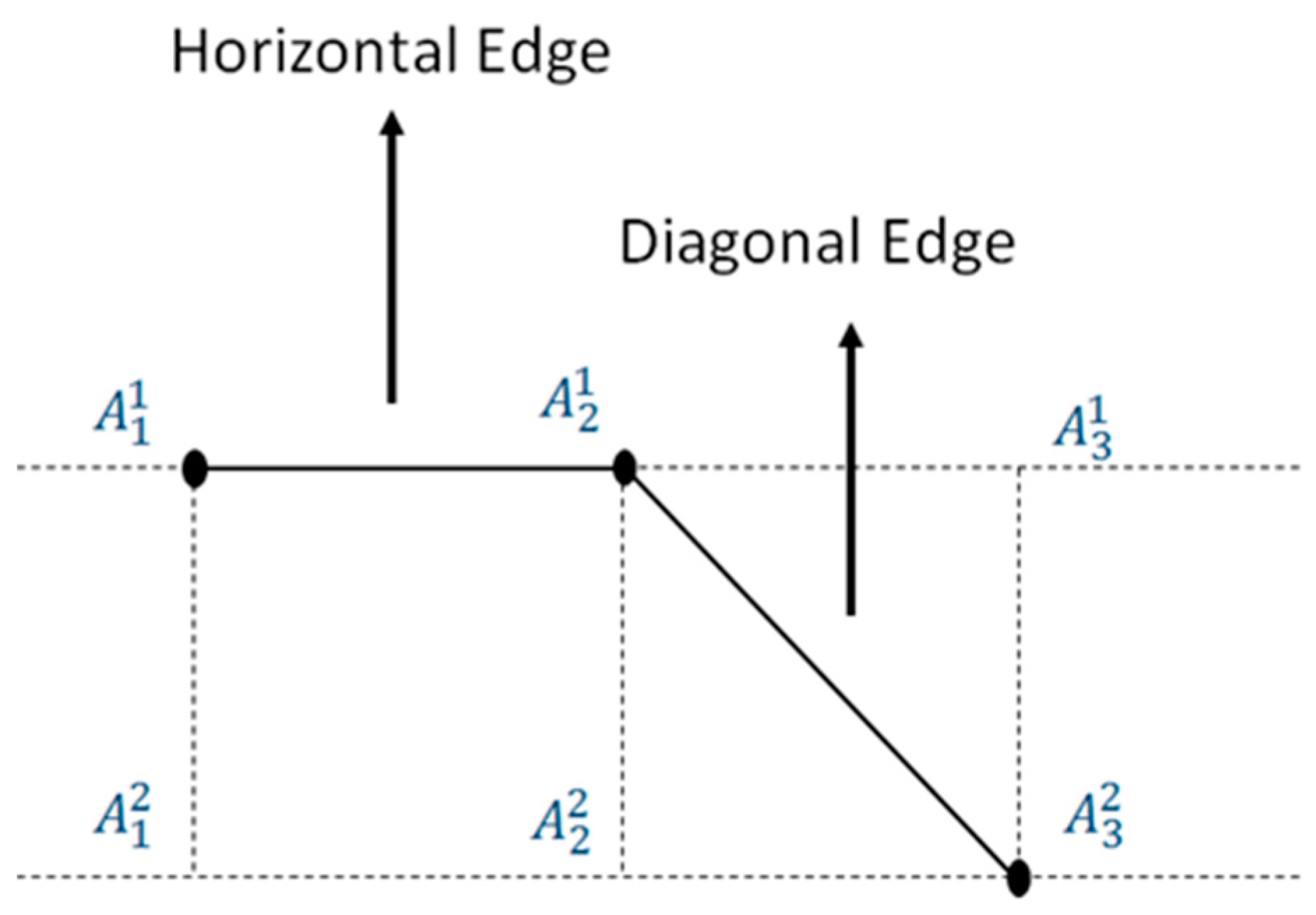
• The homeomorphism between two components of the same version is presented as a horizontal edge, whereas the homeomorphism between two components of two different versions is represented by a diagonal edge (see Figure 8). These arrangements are necessary to produce the graph of pseudo degree zero.
  

  Figure 8. Generated element $\left\{A_1^1, A_2^1, A_3^2\right\}$ on $\ast FTT{M}_3^2$grid.

Furthermore, Zilullah et al. [2] introduced some operations and properties with respect to the FTTM grid. They are recalled, summarized and listed below for convenience. Then, we will move on to the next main section of the paper wherein Conjecture 1 is finally proven as a theorem.

Definition 8.

Let$F\in G\left(\ast FTT{M}_n^k\right)$and$F=\left\{A_1^{m_1},A_2^{m_2}, \dots ,A_n^{m_n}\right\}$. A block$B$ , where $B\subseteq F$ is defined as

$$B=\left\{A_i^{m_i},A_{i+1}^{m_{i+1}},A_{i+2}^{m_{i+2}},\dots , A_{i+j}^{m_{i+j}}\right\}, 1\le i<n, 0<j\le n-1$$

(11)

$B\left(G\left(\ast FTT{M}_n^k\right)\right)$ is the set of FTTM blocks that can be generated from $G\left(\ast FTT{M}_n^k\right)$.

Definition 9.

The function$C_i^j$is defined as$C:G\left(\ast FTT{M}_n^k\right)\to B\left(G\left(\ast FTT{M}_n^k\right)\right)$for$F\in G\left(\ast FTT{M}_n^k\right)$,

$$B=\left\{A_i^{m_i},A_{i+1}^{m_{i+1}},A_{i+2}^{m_{i+2}},\dots , A_{i+j}^{m_{i+j}}\right\}, 1\le i<n, 0<j\le n-1$$

(12)

for$1<i<j<n$, where$F=\left\{A_1^{m_1},A_2^{m_2},A_3^{m_3},\dots , A_n^{m_n}\right\}$.

Definition 10.

The operation$\oplus$is a mapping$\oplus :B\left(G\left(\ast FTT{M}_n^k\right)\right)\times B\left(G\left(\ast FTT{M}_n^k\right)\right)\to B\left(G\left(\ast FTT{M}_n^k\right)\right)$such that

$$\left\{A_i^{m_i},A_{i+1}^{m_{i+1}}, \dots ,A_k^{m_k}\right\} \oplus \left\{A_p^{m_p},A_{p+1}^{m_{p+1}}, \dots ,A_j^{m_j}\right\}=\left\{A_i^{m_i},A_{i+1}^{m_{i+1}}, \dots ,A_j^{m_j}\right\}$$

(13)

when$k=p$and$m_k=m_p$, then$B_3=B_1\oplus B_2=\left\{A_i^{m_i},A_{i+1}^{m_{i+1}}, \dots ,A_j^{m_j}\right\}$.

Definition 11.

An indexed$FTTM$$\underset{j=i}{G}\left(\ast FTT{M}_n^k\right)$is defined as

$$\underset{m_j=i}{ G}\left(\ast FTT{M}_n^k\right)=\left\{F\in G\left(\ast FTT{M}_n^k\right)| A_j^{m_j}\in F,m_j=i \right\}$$

(14)

A generated $FTTM$ is then divided into blocks of three components. A set of blocks is defined as follows.

Definition 12.

A set of blocks$B_{ijk}$is defined as

$$B_{ijk}=\left\{B\in G\left(\ast FTT{M}_n^k\right)| B=\left\{A_p^{m_p},A_{p+1}^{m_{p+1}},A_{p+2}^{m_{p+2}}\right\},m_p=i,m_{p+1}=j,m_{p+2}=k\right\}$$

(15)

Since this study is concerned with graphs of pseudo degree zero, the sets that need to be taken into consideration are the ones with diagonal paths, namely, $B_{121},B_{121},B_{123},B_{131},B_{132},B_{212},B_{213},B_{232},B_{231},B_{321},B_{312},B_{323} \mathrm{and} B_{313}$.

Lemma 1.

Let$F\in \ast FTT{M}_n^k$and$F=\left\{A_1^{m_1},A_2^{m_2}, \dots ,A_n^{m_n}\right\}$. For any$A_j^{m_j}\in F$, $1<j<n$, then${\mathit{deg}}_p\left(A_j^{m_j}\right)=0$if$A_j^{m_j}$is connected to$A_{j-1}^{m_{j-1}}$and$A_{j+1}^{m_{j+1}}$by a diagonal path.

Theorem 3.

If$F\in G_d\left(\ast FTT{M}_n^3\right)$, where$G_d\left(\ast FTT{M}_n^3\right)$is the set of generated$FTTM$s with a diagonal path, then${\mathit{deg}}_{p}G\left(F\right)=2 or 0$.

Corollary 1.

The element of$G_0\left(FTT{M}_n^k\right)$has a$FTTM$path with the following properties:

• All the edges connecting the path are diagonal.
• The starting and the end points of the path belong to different versions of FTTM.

Theorem 4.

If$x\in B\left(G_0\left(\ast FTT{M}_n^k\right)\right)$, then all the paths for$x$are diagonals.

Proposition 1.

If$F \in G\left(\ast FTT{M}_n^k\right)$, then$C_1^{n-2}\left(F\right)\in G\left(\ast FTT{M}_{n-2}^k\right)$.

Lemma 2.

If$F\in G\left(\ast FTT{M}_n^k\right)$, then$\exists x,y$such that$x\in G\left(\ast FTT{M}_{n-2}^k\right), y\in C_{n-2}^n\left(G\left(\ast FTT{M}_n^k\right)\right)$and$F=x\oplus y$.

Lemma 3.

If$F \in G\left(\ast FTT{M}_n^k\right)$, then$\exists$unique tuple$\left(x,y\right)$such that$x\in G\left(\ast FTT{M}_{n-2}^k\right), y\in C_{n-2}^n\left(G\left(\ast FTT{M}_n^k\right)\right)$and$F=x\oplus y$.

Theorem 5.

If$H\subseteq G\left(\ast FTT{M}_n^k\right)$and$K=\left\{\left(x,y\right)|x\oplus y\in H, x\in G\left(\ast FTT{M}_{n-2}^3\right), y\in C_{n-2}^n\left(G\left(\ast FTT{M}_n^3\right)\right)\right\}$, then$\left|K\right|=\left|C\right|$.

Lemma 4.

$$\left({\ast \mathit{FTTM}}_n^3\right)=\underset{m_{n-2}=1}{G}\left({\ast \mathit{FTTM}}_n^3\right){{\displaystyle \cup }}^{ }\underset{m_{n-2}=2}{G}\left({\ast \mathit{FTTM}}_n^3\right){{\displaystyle \cup }}^{ }\underset{m_{n-2}=3}{G}\left({\ast \mathit{FTTM}}_n^3\right).$$

(16)

Lemma 5.

$$\underset{m_{n-2}=a}{G}\left(\ast FTT{M}_n^3\right){{\displaystyle \cap }}^{ }\underset{m_{n-2}=b}{G}\left(\ast FTT{M}_n^3\right)=\varnothing$$

(17)

for any$a,b\in \mathbb{Z}$and$a\ne b$.

Theorem 6.

$$\left|G\left(\ast FTT{M}_n^3\right)\right|=\left|\underset{m_{n-2}=1}{G}\left(\ast FTT{M}_n^3\right)\right|+\left|\underset{m_{n-2}=2}{G}\left(\ast FTT{M}_n^3\right)\right|+\left|\underset{m_{n-2}=3}{G}\left(\ast FTT{M}_n^3\right)\right|$$

(18)

5. The Theorem

All the materials laid down in previous sections are assembled to produce the analytical proof of Conjecture 1. The first step is to find $\left|G_d\left(\ast FTT{M}_n^3\right)\right|$since $G_0\left(\ast FTT{M}_n^3\right)$ is a subset of $G_d\left(\ast FTT{M}_n^3\right)$ by Theorem 2.

Theorem 7.

$$\left|G_d\left(\ast FTT{M}_n^3\right)\right|=\{\begin{array}{l}12 . 4^{\frac{n-3}{2}}, n is odd, n\ge 3\\ 6 . 4^{\frac{n-2}{2}}, n is even , n\ge 4.\end{array}$$

(19)

Proof of Theorem 7.

(By mathematical induction)

Let

$$P\left(m\right)=\left|G_d\left(\ast FTT{M}_n^3\right)\right|=\{\begin{array}{l}12 . 4^{\frac{n-3}{2}}, n is odd, n\ge 3\\ 6 . 4^{\frac{n-2}{2}}, n is even , n\ge 4\end{array}$$

(20)

For odd numbers, $P\left(3\right):n=3,$

$$P\left(3\right)=\left|G_d\left(\ast FTT{M}_3^3\right)\right|=12 . 4^{\frac{3-3}{2}}=12.$$

(21)

There are exactly 12 combinations, namely

$$\begin{gathered} \left\{A_1^1,A_2^2,A_3^3\right\},\left\{A_1^1,A_2^2,A_3^1\right\},\left\{A_1^1,A_2^3,A_3^2\right\},\left\{A_1^1,A_2^3,A_3^1\right\},\left\{A_1^2,A_2^1,A_3^3\right\},\left\{A_1^2,A_2^3,A_3^1\right\}, \\ \left\{A_1^2,A_2^1,A_3^2\right\},\left\{A_1^2,A_2^3,A_3^1\right\},\left\{A_1^3,A_2^2,A_3^3\right\},\left\{A_1^3,A_2^2,A_3^1\right\},\left\{A_1^3,A_2^1,A_3^3\right\},\left\{A_1^3,A_2^1,A_3^2\right\} \end{gathered}$$

Now assume $P\left(m=2k+1\right):n=2k+1$ is true with

$$P\left(m\right)=\left|G_d\left(\ast FTT{M}_{2k+1}^3\right)\right|=12 . 4^{\frac{2k+1-3}{2}}=12 . 4^{k-1}$$

(22)

for $P\left(\begin{array}{c}m+2=2k+1+2\\ 2k+3\end{array}\right)$.

By using Theorem 4, $P\left(m+1\right)=\left|G_0\left(\ast FTT{M}_{2k+3}^3\right)\right|=\left|K\right|$ such that

$$K=\left\{\left(x,y\right)|x\oplus y\in H, x\in G\left(\ast FTT{M}_{2k+1}^3\right), y\in C_{n-2}^n\left(G\left(\ast FTT{M}_{2k+3}^3\right)\right)\right\}.$$

(23)

By using Theorem 5,

$$\begin{array}{ll}\left|P\left(m+1\right)\right|& =\left|G_d\left(\ast FTT{M}_{2k+3}^3\right)\right|\\ & =\left|\underset{m_{n-2}=1}{G_d}\left(\ast FTT{M}_{2k+3}^3\right)\right|+\left|\underset{m_{n-2}=2}{G_d}\left(\ast FTT{M}_{2k+3}^3\right)\right|+\left|\underset{m_{n-2}=3}{G_d}\left(\ast FTT{M}_{2k+3}^3\right)\right| \end{array}$$

(24)

The set$\underset{m_{n-2}=1}{G_d}\left(\ast FTT{M}_{2k+3}^3\right)$ can be constructed from $\left(x,y\right)$ where $x\in \underset{m_{n-2}=1}{G_d}\left(\ast FTT{M}_{2k+1}^3\right)$ and $y\in C_{n-2}^n\left(G_d\left(\ast FTT{M}_{2k+3}^3\right)\right)$. There are four options for $y$, namely $B_{121},B_{123}, B_{131}, \mathrm{and} B_{132}$. Hence,

$$\left|\underset{m_{n-2}=1}{G_d}\left(\ast FTT{M}_{2k+3}^3\right)\right|=4\left|\underset{m_{n-2}=1}{G_d}\left(\ast FTT{M}_{2k+1}^3\right)\right|.$$

(25)

The same process can be applied to $\left|\underset{m_{n-2}=2}{G_d}\left(\ast FTT{M}_{2k+3}^3\right)\right|$ and $\left|\underset{m_{n-2}=3}{G_d}\left(\ast FTT{M}_{2k+3}^3\right)\right|$. Thus,

$$\begin{array}{c}\left|P\left(m+1\right)\right|\hfill \\ =\left|G_d\left(\ast FTT{M}_{2k+3}^3\right)\right|\hfill \\ =4\left|\underset{m_{n-2}=1}{G_d}\left(\ast FTT{M}_{2k+1}^3\right)\right|+4\left|\underset{m_{n-2}=2}{G_d}\left(\ast FTT{M}_{2k+1}^3\right)\right|+4\left|\underset{m_{n-2}=3}{G_d}\left(\ast FTT{M}_{2k+1}^3\right)\right|\hfill \\ =4\left(\left|\underset{m_{n-2}=1}{G_d}\left(\ast FTT{M}_{2k+1}^3\right)\right|+\left|\underset{m_{n-2}=2}{G_d}\left(\ast FTT{M}_{2k+1}^3\right)\right|+\left|\underset{m_{n-2}=3}{G_d}\left(\ast FTT{M}_{2k+1}^3\right)\right|\right)\hfill \\ =4\left|G_d\left(\ast FTT{M}_{2k+1}^3\right)\right|=4 . 12 . 4^{k-1}=12 . 4^k.\hfill \end{array}$$

(26)

Similarly, the same induction process can be used as proof for even parts. □

The set $G_d\left(\ast FTT{M}_n^3\right)$ has only two possible subsets, namely $G_0\left(\ast FTT{M}_n^3\right)$ and $H_n=\left\{x\in G_d\left(\ast FTT{M}_n^3\right)|{\mathit{deg}}_{p}x=2\right\}$. To find $G_0\left(\ast FTT{M}_n^3\right)$, the relation between $G_0\left(\ast FTT{M}_n^3\right)$, $G_d\left(\ast FTT{M}_n^3\right)$ and $H_n$ must be investigated.

Lemma 6.

If$H_n=\left\{x\in G_d\left(\ast FTT{M}_n^3\right)|{\mathit{deg}}_{p}x=2\right\}$, then$\left|H_n\right|=\left|G_d\left(\ast FTT{M}_n^3\right)\right|-\left|G_0\left(\ast FTT{M}_n^3\right)\right|.$

Proof of Lemma 6.

Let $x\in G_d\left(\ast FTT{M}_n^3\right)$, then ${\mathit{deg}}_p\left(x\right)=0$ or ${\mathit{deg}}_p\left(x\right)=2$ by Theorem 5. Thus, $x\in G_0\left(\ast FTT{M}_n^3\right)$ or $x\in H_n$, i.e., $\left|G_d\left(\ast FTT{M}_n^3\right)\right|=\left|G_0\left(\ast FTT{M}_n^3\right)\right|+\left|H_n\right|$ or $\left|H_n\right|=\left|G_d\left(\ast FTT{M}_n^3\right)\right|-\left|G_0\left(\ast FTT{M}_n^3\right)\right|$. □

Finally, $\left|\underset{m_{n-2}=i}{G_0}\left(\ast FTT{M}_n^3\right)\right|$ is determined using Lemma 6 and Theorem 5.

Theorem 8.

$$\left|\underset{m_{n-2}=i}{G_0}\left(\ast FTT{M}_n^3\right)\right|=3\left|\underset{m_{n-2}=i}{G_0}\left(\ast FTT{M}_{n-2}^3\right)\right|+2\left|H_{n-2}\right|, n>4$$

(27)

Proof of Theorem 8.

By Theorem 5, $\left|\underset{m_{n-2}=i}{G_0}\left(\ast FTT{M}_n^3\right)\right|$ can be determined by the combination of $\left(x,y\right)$ where $x\oplus y\in \underset{m_{n-2}=i}{G_0}\left(\ast FTT{M}_n^3\right),x\in \underset{m_{n-2}=i}{G}\left(\ast FTT{M}_{n-2}^3\right),y\in C_{n-2}^n\left(\underset{m_{n-2}=i}{G}\left(\ast FTT{M}_{n-2}^3\right)\right)$. By Theorem 4, all $x$ edges must be diagonal; hence, $x\in \underset{m_{n-2}=i}{G_d}\left(\ast FTT{M}_{n-2}^3\right)$. There are two possibilities for the value of $x$, namely $x\in \underset{m_{n-2}=i}{G_0}\left(\ast FTT{M}_{n-2}^3\right)$ or $x\in \left|H_{n-2}\right|$, where $H_{n-2}=\left\{x\in G_d\left(\ast FTT{M}_{n-2}^3\right)| {\mathit{deg}}_p x=2\right\}$ from Theorem 3. Case $i=1$: if $x\in \underset{m_{n-2}=1}{G_0}\left(\ast FTT{M}_{n-2}^3\right)$, then $A_1^{m_1}\in x , m_1\ne 1$ which implies $m_1=2$ or $m_1=3$ by Corollary 1.

Let $X_2=\left\{x\in \underset{m_{n-2}=1}{G_0}\left(\ast FTT{M}_{n-2}^3\right)|m_1=2 \right\}$, $X_3=\left\{x\in \underset{m_{n-2}=1}{G_0}\left(\ast FTT{M}_{n-2}^3\right)|m_1=3 \right\}$, then for any $x\in X_2$, then $y\in B_{121},B_{123},B_{131}$and also for any $x\in X_3$, then $y\in B_{121},B_{132},B_{131}$by Corollary 1. Thus, for $\in \underset{m_{n-2}=1}{G_0}\left(\ast FTT{M}_{n-2}^3\right)$, there are $3\left|\underset{m_{n-2}=1}{G_0}\left(\ast FTT{M}_{n-2}^3\right)\right|$ combinations of tuple $\left(x,y\right)$.

If $x\in H_{n-2}$, then $A_1^{m_1}\in x , m_1=1$ when $x\in H_{n-2}$ and $y\in B_{123},B_{132}$ by Corollary 1. Thus, there are $3\left|H_{n-2}\right|$ combinations of tuple $\left(x,y\right)$ Hence, $\left|\underset{m_{n-2}=1}{G_0}\left(\ast FTT{M}_n^3\right)\right|=3\left|\underset{m_{n-2}=1}{G_0}\left(\ast FTT{M}_{n-2}^3\right)\right|+2\left|H_{n-2}\right|, n>4$. Using the same procedure as for $i=1$, the same result can be obtained for $i=2,3$. □

Theorem 9.

$$\left|G_0\left(\ast FTT{M}_n^3\right)\right|=\{\begin{array}{l}\left|G_0\left(\ast FTT{M}_{n-2}^3\right)\right|+3. 2^{n-2}, n is odd, n>3\\ \left|G_0\left(\ast FTT{M}_{n-2}^3\right)\right|+3. 2^n, n is even, n>4\end{array}$$

(28)

where$\left|G_0\left(\ast FTT{M}_3^3\right)\right|=6$,$\left|G_0\left(\ast FTT{M}_4^3\right)\right|=12$.

Proof of Theorem 9.

Using Theorem 6, $\left|G_0\left(\ast FTT{M}_n^3\right)\right|=\left|\underset{m_{n-2}=1}{G_0}\left(\ast FTT{M}_n^3\right)\right|+\left|\underset{m_{n-2}=2}{G_0}\left(\ast FTT{M}_n^3\right)\right|+\left|\underset{m_{n-2}=3}{G_0}\left(\ast FTT{M}_n^3\right)\right|$. From Theorem 8 and Lemma 6,

$$\begin{array}{l}\left|G_0\left(\ast FTT{M}_n^3\right)\right| \\ =\left|\underset{m_{n-2}=1}{G_0}\left(\ast FTT{M}_{n-2}^3\right)\right|+2\left|\underset{m_{n-2}=1}{G_d}\left(\ast FTT{M}_{n-2}^3\right)\right|+\left|\underset{m_{n-2}=2}{G_0}\left(\ast FTT{M}_{n-2}^3\right)\right|+2\left|\underset{m_{n-2}=2}{G_d}\left(\ast FTT{M}_{n-2}^3\right)\right|+\left|\underset{m_{n-2}=3}{G_0}\left(\ast FTT{M}_{n-2}^3\right)\right|+2\left|\underset{m_{n-2}=3}{G_d}\left(\ast FTT{M}_{n-2}^3\right)\right|\end{array}$$

$$\begin{array}{l}=\left(\left|\underset{m_{n-2}=1}{G_0}\left(\ast FTT{M}_{n-2}^3\right)\right|+\left|\underset{m_{n-2}=2}{G_0}\left(\ast FTT{M}_{n-2}^3\right)\right|+\left|\underset{m_{n-2}=3}{G_0}\left(\ast FTT{M}_{n-2}^3\right)\right|\right)+2\left(\left|\underset{m_{n-2}=3}{G_d}\left(\ast FTT{M}_{n-2}^3\right)\right|+\left|\underset{m_{n-2}=1}{G_d}\left(\ast FTT{M}_{n-2}^3\right)\right|+\left|\underset{m_{n-2}=2}{G_d}\left(\ast FTT{M}_{n-2}^3\right)\right|\right)\\ =\left|G_0\left(\ast FTT{M}_{n-2}^3\right)\right|+2\ast \left|G_d\left(\ast FTT{M}_n^3\right)\right|.\end{array}$$

(29)

Hence by Theorem 7,

$$\left|G_0\left(\ast FTT{M}_n^3\right)\right|=\{\begin{array}{cc}\hfill \left|G_0\left(\ast FTT{M}_{n-2}^3\right)\right|+3 . 2^{n-2},\hfill & n is odd, n>3\hfill \\ \hfill \left|G_0\left(\ast FTT{M}_{n-2}^3\right)\right|+3 . 2^n,\hfill & n is even , n>4\hfill \end{array}$$

(30)

such that $\left|G_0\left(\ast FTT{M}_3^3\right)\right|=6, \left|G_0\left(\ast FTT{M}_4^3\right)\right|=12$. □

Theorem 9 is another version of the earlier conjecture. A simple algebraic manipulation is needed to show their equivalence. We formally state and prove this as the final theorem.

Theorem 10.

$$\begin{array}{cc}\hfill \left|G_0^3\left(FTT{M}_n^3\right)\right|& =\{\begin{array}{l}4\left|G_0^3\left(FTT{M}_{n-2}^3\right)\right|+12 , where n is even \\ 4\left|G^3{ }_0\left(FTT{M}_{n-2}^3\right)\right|+6, where n is odd\end{array}\hfill \\ & =\{\begin{array}{l}\left|G_0\left(\ast FTT{M}_{n-2}^3\right)\right|+3 . 2^{n-2}, n is odd, n>3\\ \left|G_0\left(\ast FTT{M}_{n-2}^3\right)\right|+3 . 2^n, n is even , n>4\end{array} \hfill \end{array}$$

(31)

where,$\left|G_0\left({\ast \mathit{FTTM}}_3^3\right)\right|=6,\left|G_0\left(\ast FTT{M}_4^3\right)\right|=12$.

Proof of Theorem 10.

By Theorem 9,

$$\left|G_0\left(FTT{M}_n^3\right)\right|=\{\begin{array}{c}4\left|G_0\left(FTT{M}_{n-2}^3\right)\right|+12 , where n is even \\ 4\left|G_0\left(FTT{M}_{n-2}^3\right)\right|+6, where n is odd\end{array}$$

(32)

and $\left|G_0\left({\mathit{FTTM}}_3^3\right)\right|=6$, $\left|G_0\left({\mathit{FTTM}}_4^3\right)\right|=12$.

However, when n is odd,

$$\begin{array}{cc}\hfill \left|G_0\left(FTT{M}_5^3\right)\right|& =4 . 6+6\hfill \\ & =4^1 . 6+4^0 . 6\hfill \\ \hfill \left|G_0\left(FTT{M}_7^3\right)\right|& =4\left(4 . 6+6\right)+6\hfill \\ & =4^2 . 6+4^1 . 6+4^0 . 6\hfill \\ \hfill \left|G_0\left(FTT{M}_9^3\right)\right|& =4\left(4\left(4 . 6+6\right)+6\right)+6\hfill \\ & =4^3 . 6+4^2 . 6+4^1 . 6+4^0 . 6\hfill \\ \hfill \left|G_0\left(FTT{M}_{11}^3\right)\right|& =4\left(4\left(4\left(4 . 6+6\right)+6\right)+6\right)+6\hfill \\ & =4^4 . 6+4^3 . 6+4^2 . 6+4^1 . 6+4^0 . 6 \hfill \end{array}$$

(33)

Thus, $\left|G_0\left(FTT{M}_n^3\right)\right|={{\displaystyle \sum }}_{k=0}^{\frac{n-3}{2}}{4}^k . 6$.

Notice that

$$\begin{array}{cc}\hfill \left|G_0\left(FTT{M}_n^3\right)\right|& ={\displaystyle {\displaystyle \sum }_{k=0}^{\frac{n-3}{2}}}{4}^k . 6\hfill \\ & =4^{\frac{n-3}{2}} . 6+{\displaystyle {\displaystyle \sum }_{k=0}^{\frac{n-5}{2}}}{4}^k . 6\hfill \\ & =2^{n-3} . 6+\left|G_0\left(FTT{M}_{n-2}^3\right)\right|\hfill \\ & =2^{n-2} . 3+\left|G_0\left(FTT{M}_{n-2}^3\right)\right| \hfill \end{array}$$

(34)

When n is even,

$$\begin{array}{cc}\hfill \left|G_0\left(FTT{M}_6^3\right)\right|& =4 . 12+12\hfill \\ & =4^1 . 12+4^0 . 12\hfill \\ \hfill \left|G_0\left(FTT{M}_8^3\right)\right|& =4\left(4 . 12+12\right)+12\hfill \\ & =4^2 . 12+4^1 . 12+4^0 . 12\hfill \\ \hfill \left|G_0\left(FTT{M}_{10}^3\right)\right|& =4\left(4\left(4 . 12+12\right)+12\right)+12\hfill \\ & =4^3 . 12+4^2 . 12+4^1 . 12+4^0 . 12\hfill \\ \hfill \left|G_0\left(FTT{M}_{12}^3\right)\right|& =4\left(4\left(4\left(4 . 12+12\right)+12\right)+12\right)+12\hfill \\ & =4^4 . 12+4^3 . 12+4^2 . 12+4^1 . 12+4^0 . 12 \hfill \end{array}$$

(35)

Thus, $\left|G_0\left(FTT{M}_n^3\right)\right|={\displaystyle \sum }_{k=0}^{\frac{n-4}{2}}{4}^k . 12$.

Notice that,

$$\begin{array}{ll}\left|G_0\left(FTT{M}_n^3\right)\right|& = {\displaystyle {\displaystyle \sum }_{k=0}^{\frac{n-4}{2}}}{4}^k . 12\hfill \\ & =4^{\frac{n-4}{2}} . 12+{\displaystyle {\displaystyle \sum }_{k=0}^{\frac{n-6}{2}}}{4}^k . 12\\ & =2^{n-2} . 3+{\displaystyle {\displaystyle \sum }_{k=0}^{\frac{n-6}{2}}}{4}^k . 12\\ & =2^{n-2} . 3+\left|G_0\left(FTT{M}_{n-2}^3\right)\right|\end{array}$$

(36)

It shows that the equation in Theorem 9 is exactly the statement of the conjecture. In other words, the conjecture is proven by construction. □

The whole process of proving Conjecture 1 is summarized below in Figure 9.

Figure 9. Outline of proving Conjecture 1 by construction.

6. Conclusions

The developed grid-based method of proof is new; some definitions and properties were introduced, whereas others were investigated along the way. The originality and advantages of this method can be summarized in the point forms below.

• It provides a different perspective to the structure of $\mathit{FTTM}$. Instead of a polygon representation for each version of $FTTM$, a straight line is now used. The components of $FTT{M}_n$ are arranged on a horizontal line of vertices and the lines represent the homeomorphisms between the components of $FTT{M}_n$.
• A vertical line is added to represent a homeomorphism between two components of different versions; hence, a grid is created.
• It is represented in two dimensions; therefore, it reduces the complexity of the structure.
• The process of adding a new component is easier than in a sequence of polygon.
• It can take any number of components by adding the number of vertices at the end of the grid.
• The homeomorphism between two components of the same version is presented as a horizontal edge, whereas the homeomorphism between two components of two different versions is represented by a diagonal edge (see Figure 8).
• This grid-based technique offers an edge in proving the conjecture; in particular, it enables one to visualize a given problem in a 2-dimensional space.
• Finally, the conjecture that spells the number of the generated FTTM graph of pseudo degree zero with respect to n number of components and k number of versions is proven analytically for the first time using this method.

However, the lengthy computing time for simulation needs to be resolved for larger k and n, accordingly. This may be overcome by employing parallel computing, and the grid-based technique can be very handy for such enumerative combinatorics problems in the near future.