Non-Separable Linear Canonical Wavelet Transform

Abstract

This study aims to achieve an efficient time-frequency representation of higher-dimensional signals by introducing the notion of a non-separable linear canonical wavelet transform in $L^2\left({\mathbb{R}}^n\right)$. The preliminary analysis encompasses the derivation of fundamental properties of the novel integral transform including the orthogonality relation, inversion formula, and the range theorem. To extend the scope of the study, we formulate several uncertainty inequalities, including the Heisenberg’s, logarithmic, and Nazorav’s inequalities for the proposed transform in the linear canonical domain. The obtained results are reinforced with illustrative examples.

1. Introduction

The origin of the multi-dimensional linear canonical transform (LCT) dates back to the early 1970s with the foundational work of Moshinsky and Quesne [1] in quantum mechanics to study the linear maps of phase space. Soon after its inception in quantum mechanics, the linear canonical transform has been exclusively studied both in theory and applications [2,3]. The theory of multi-dimensional non-separable LCT involving a general $2n\times 2n$ real, symplectic matrix $\mathbf{M}=(A,B:C,D)$ with $n(2n+1)$ independent parameters offers a canonical formalism for the representation of several physical systems in a lucid and insightful way. For any $f\in L^2\left({\mathbb{R}}^n\right)$, the non-separable LCT with respect to a real, symplectic matrix $\mathbf{M}$ is given by [4,5]

$$\begin{array}{c}\hfill {\mathcal{F}}^{\mathbf{M}}\left[f\right]\left(\mathbf{w}\right)={\displaystyle \frac{1}{{|detB|}^{1/2}}}{\int }_{{\mathbb{R}}^n}f\left(\mathbf{t}\right)e^{i\pi \left({\mathbf{w}}^{T}D{B}^{-1}\mathbf{w}-2{\mathbf{w}}^T{B}^{T^{-1}}\mathbf{t}+{\mathbf{t}}^T{B}^{-1}A\mathbf{t}\right)}d\mathbf{t},\left|detB\right|\ne 0.\end{array}$$

(1)

The importance of the arbitrary real symplectic matrices involved in Equation (1) lies in the fact that an appropriate choice of the matrix can be taken to inculcate a sense of rotation and shift into both the time and frequency axes, resulting in an efficient representation of the chirp-like signals, which are ubiquitous both in nature and man-made systems. Due to the extra degrees of freedom, the non-separable LCT has been successfully employed in diverse problems arising in various branches of science and engineering, such as harmonic analysis, reproducing kernel Hilbert spaces, optical systems, quantum mechanics, sampling, image processing, and so on [6,7].

Undoubtedly, wavelet transforms have fascinated the scientific, engineering, and research communities both with their versatile applicability and lucid mathematical framework [8,9]. In recent years, the classical wavelet transform has been extended and employed in different domains. The most prompt ones are the fractional wavelet transform [10], linear canonical wavelet transform [11,12], special affine wavelet transform [13,14], quaternion linear canonical wavelet transform [15], and quadratic-phase wavelet transform [16]. Unfortunately, all these transforms only perform well at representing point singularities and are incompetent at handling the distributed singularities, such as curves or edges in higher-dimensional signals [17,18,19,20]. The intuitive reason for this inadequacy is that wavelets are isotropic entities generated by isotropically dilating the mother wavelet, and as such, they ignore the geometric properties of the structures to be analyzed. Therefore, the conventional wavelet approach is inadequate while dealing with multi-dimensional signals, wherein the primary interest is to efficiently capture the geometric features, such as edges and corners, appearing due to the spatial occlusion between different objects. As such, the key problem in multi-dimensional signal analysis is to extract and characterize the relevant geometric information regarding the occurrence of curves and boundaries in signals. Subsequently, a higher-dimensional variant of the standard wavelet transform has been proposed, which serves as a potent tool for representing non-transient multi-dimensional signals in the time-frequency domain. Mathematically, the multi-dimensional wavelet transform of any $f\in L^2\left({\mathbb{R}}^n\right)$ is defined by [21]

$$\begin{array}{c}\hfill {\mathcal{W}}_{\psi }\left[f\right](a,\mathbf{b})={\displaystyle \frac{1}{\sqrt{a}}}{\int }_{{\mathbb{R}}^n}f\left(\mathbf{t}\right)\overline{\psi \left({\displaystyle \frac{\mathbf{t}-\mathbf{b}}{a}}\right)}{e}^{-i\mathbf{w}·\mathbf{t}}d\mathbf{t},a\in {\mathbb{R}}^{+},\mathbf{b}\in {\mathbb{R}}^n,\end{array}$$

(2)

where a is called the scaling parameter, which controls the degree of compression or scale, and $\mathbf{b}$ is the translation parameter that determines the time location of the wavelet. The multi-dimensional wavelet transform in Equation (2) has found numerous applications across diverse fields of science and engineering, particularly in video image processing, medical imaging, singular detection problems, fluid dynamics, shape recognition, and so on [21,22]. In the context of higher-dimensional wavelet theory, the symmetry property of wavelets is often desirable in practical applications, and as such, wavelets can reveal different patterns and singularities of highly nonstationary signals, such as Brownian motions, patterns on the water surfaces, fractal properties of the velocity field, computations of Renyi dimensions, Hurst and H¨older exponents. Some prominent examples of the symmetric wavelets include biorthogonal wavelets, quincunx wavelets, and carinal B-splines.

Keeping in view the profound characteristics of the multi-dimensional wavelet transform and more degrees of freedom of non-separable linear canonical transforms, we are deeply motivated to intertwine these integral transforms into a novel integral transform coined as a non-separable linear canonical wavelet transform. The novel integral transform can efficiently localize any non-transient signal in the time-frequency plane with more degrees of freedom. With major modifications to the existing multi-dimensional wavelet transform in Equation (2), we propose the non-separable linear canonical wavelet transform of any $f\in L^2\left({\mathbb{R}}^n\right)$ concerning the free symplectic matrix $\mathbf{M}=\left(A,B:C,D\right)$ as

$$\begin{array}{c}\hfill {\mathcal{W}}_{\psi }^{\mathbf{M}}\left[f\right](a,\mathbf{b})={\displaystyle \frac{1}{{|detB|}^{1/2}}}{\int }_{{\mathbb{R}}^n}f\left(\mathbf{t}\right)\overline{\psi \left({\displaystyle \frac{\mathbf{t}-\mathbf{b}}{a}}\right)}{e}^{-\pi i\left({\Lambda }_a^{T}D{B}^{-1}{\Lambda }_a-2{\Lambda }_a^T{B}^{T^{-1}}\mathbf{t}+{\mathbf{t}}^T{B}^{-1}A\mathbf{t}\right)}d\mathbf{t},\end{array}$$

(3)

where ${\Lambda }_a={(aa\dots a)}^T$. Besides studying all the fundamental properties of the novel wavelet transform, we derive some well-known theorems, including the Rayleigh’s theorem, inversion formula, and range theorem. In the sequel, we also formulate several uncertainty inequalities such as the Heisenberg’s, logarithmic, and Nazorav-type inequalities for the non-separable linear canonical wavelet transform in Equation (3).

The rest of the article is structured as follows: Section 2 is concerned with the preliminary aspects of the study and the formulation of the non-separable linear canonical wavelet transform. Section 3 is devoted to formulating several variants of the uncertainty principles, such as Heisenberg’s, logarithmic, and Nazorav-type inequalities, for the proposed transform. Finally, a conclusion is extracted in Section 4.

2. Non-Separable Linear Canonical Wavelet Transform in $L^2\left({\mathbb{R}}^n\right)$

In this section, we first provide a healthy overview of the non-separable linear canonical transform. Then, we introduce the notion of the non-separable linear canonical wavelet transform in $L^2\left({\mathbb{R}}^n\right)$, followed by some fundamental properties of the proposed transform, including the orthogonality relation, energy preserving relation, range theorem, and the inversion formula.

2.1. Non-Separable Linear Canonical Transform

For typographical convenience, we shall denote a real $2n\times 2n$ matrix

$$\begin{array}{c}\hfill \mathbf{M}=\left(\begin{array}{cc}A& B\\ C& D\end{array}\right)=\left(\begin{array}{cccccccc}{a}_{11}& a_{12}& \cdots & a_{1n}& b_{11}& b_{12}& \cdots & b_{1n}\\ a_{21}& a_{22}& \cdots & a_{2n}& b_{21}& b_{22}& \cdots & b_{2n}\\ ⋮& ⋮& \ddots & ⋮& ⋮& ⋮& \ddots & ⋮\\ a_{n1}& a_{n2}& \cdots & a_{nn}& b_{n1}& b_{n2}& \cdots & b_{nn}\\ c_{11}& c_{12}& \cdots & c_{1n}& d_{11}& d_{12}& \cdots & d_{1n}\\ c_{21}& c_{22}& \cdots & c_{2n}& d_{21}& d_{22}& \cdots & d_{2n}\\ ⋮& ⋮& \ddots & ⋮& ⋮& ⋮& \ddots & ⋮\\ c_{n1}& c_{n2}& \cdots & c_{nn}& d_{n1}& d_{n2}& \cdots & d_{nn}\end{array}\right)\end{array}$$

(4)

as $\mathbf{M}=\left(A,B:C,D\right)$, where $A,B,C$, and D are $n\times n$ sub-matrices with real entries. Moreover, the matrix $\mathbf{M}=\left(A,B:C,D\right)$ is said to be free symplectic if ${\mathbf{M}}^T\mathbf{J}\mathbf{M}=\mathbf{J}$ and $\left|detB\right|\ne 0$, where $\mathbf{J}=\left(\mathbf{0},I_n:-I_n,\mathbf{0}\right)$, and $I_n$ denotes the n-dimensional identity matrix. Furthermore, the sub-matrices corresponding to the free symplectic matrix $\mathbf{M}=(A,B:C,D)$ satisfy

$$\begin{array}{c}\hfill A{B}^T=B{A}^T,C{D}^T=D{C}^T,A{D}^T-B{C}^T=I_n,\end{array}$$

(5)

or equivalently

$$\begin{array}{c}\hfill A^{T}C=C^{T}A,B^{T}D=D^{T}B,A^{T}D-C^{T}B=I_n.\end{array}$$

(6)

The transpose and inverse corresponding to the free symplectic matrix $M=\left(A,B:C,D\right)$ are given by ${\mathbf{M}}^T=\left(A^T,C^T:B^T,D^T\right)$ and ${\mathbf{M}}^{-1}=\left(D^T,-B^T:-C^T,A^T\right)$, respectively. Moreover, we have

$$\begin{array}{cc}\hfill \mathbf{M}{\mathbf{M}}^{-1}& =\left(\begin{array}{cc}A& B\\ C& D\end{array}\right)\left(\begin{array}{cc}{D}^T& -B^T\\ -C^T& A^T\end{array}\right)\hfill \\ \hfill & =\left(\begin{array}{cc}A{D}^T-B{C}^T& -A{B}^T+B{A}^T\\ C{D}^T-D{C}^T& -C{B}^T+D{A}^T\end{array}\right)\hfill \\ \hfill & =\left(\begin{array}{cc}{I}_n& 0\\ 0& I_n\end{array}\right).\hfill \end{array}$$

A typical example of a $4\times 4$ free symplectic matrix is given below

$$\begin{array}{c}\hfill \mathbf{M}=\left(\begin{array}{cccc}1& 2& -1/2& -1/2\\ -2& 1& -1/2& 1/2\\ -1& -3& 1& 1\\ -1& 0& -1/2& 1/2\end{array}\right).\end{array}$$

Definition 1.

Given a free symplectic matrix $\mathbf{M}=\left(A,B:C,D\right)$, the non-separable linear canonical transform of any $f\in L^2\left({\mathbb{R}}^n\right)$ is denoted by ${\mathcal{F}}^{\mathbf{M}}\left[f\right]$ and is defined as

$$\begin{array}{c}\hfill {\mathcal{F}}^{\mathbf{M}}\left[f\right]\left(\mathbf{w}\right)={\int }_{{\mathbb{R}}^n}f\left(\mathbf{t}\right){\mathcal{K}}^{\mathbf{M}}(\mathbf{t},\mathbf{w})d\mathbf{t},\end{array}$$

(7)

where the kernel ${\mathcal{K}}^{\mathbf{M}}(\mathbf{t},\mathbf{w})$ is given by

$$\begin{array}{c}\hfill {\mathcal{K}}^{\mathbf{M}}\left(\mathbf{x},\mathbf{w}\right)={\displaystyle \frac{1}{{|detB|}^{1/2}}}exp\left\{\pi i\left({\mathbf{w}}^T{DB}^{-1}\mathbf{w}-2{\mathbf{w}}^T{B}^{T^{-1}}\mathbf{t}+{\mathbf{t}}^T{B}^{-1}A\mathbf{t}\right)\right\},\left|detB\right|\ne 0.\end{array}$$

(8)

The additive property of the non-separable LCT (Equation (7)) is very crucial for its understanding and application and is given by

$$\begin{array}{c}\hfill {\mathcal{F}}^{{\mathbf{M}}_1}\left[{\mathcal{F}}^{{\mathbf{M}}_2}\left[f\left(\mathbf{t}\right)\right]\right]\left(\mathbf{w}\right)={\mathcal{F}}^{{\mathbf{M}}_1{\mathbf{M}}_2}\left[f\left(\mathbf{t}\right)\right]\left(\mathbf{w}\right).\end{array}$$

The Plancheral and inversion formulae corresponding to Equation (7) are given by

$$\begin{array}{cc}\hfill & {⟨f,g⟩}_2={⟨{\mathcal{F}}^{\mathbf{M}}\left[f\right],{\mathcal{F}}^{\mathbf{M}}\left[g\right]⟩}_2,\forall f,g\in L^2\left({\mathbb{R}}^n\right)\mathrm{and}\hfill \end{array}$$

(9)

$$\begin{array}{cc}\hfill & f\left(\mathbf{t}\right)={\mathcal{F}}^{{\mathbf{M}}^{-1}}\left[{\mathcal{F}}^{\mathbf{M}}\left[f\right]\left(\mathbf{w}\right)\right]\left(\mathbf{x}\right)={\int }_{{\mathbb{R}}^n}{\mathcal{F}}^{\mathbf{M}}\left[f\right]\left(\mathbf{w}\right){\mathcal{K}}^{{\mathbf{M}}^{-1}}(\mathbf{w},\mathbf{t})d\mathbf{w},\hfill \end{array}$$

(10)

respectively, where ${\mathbf{M}}^{-1}=\left(D^T,-B^T:-C^T,A^T\right)$. Furthermore, the kernel in Equation (8) satisfies the following properties:

(i)

${\mathcal{K}}^{{\mathbf{M}}^{-1}}(\mathbf{w},\mathbf{t})=\overline{{\mathcal{K}}^{\mathbf{M}}(\mathbf{t},\mathbf{w})}$,

(ii)

${\displaystyle {\int }_{{\mathbb{R}}^n}{\mathcal{K}}^{\mathbf{M}}(\mathbf{t},\mathbf{w}){\mathcal{K}}^{{\mathbf{M}}^{-1}}(\mathbf{t},\mathbf{z})d\mathbf{t}=\delta (\mathbf{z}-\mathbf{w})}$,

(iii)

${\displaystyle {\int }_{{\mathbb{R}}^n}{\mathcal{K}}^{\mathbf{M}}(\mathbf{t},\mathbf{w}){\mathcal{K}}^{{\mathbf{M}}^{-1}}(\mathbf{z},\mathbf{w})d\mathbf{w}=\delta (\mathbf{z}-\mathbf{t})}$,

(iv)

${\displaystyle {\int }_{{\mathbb{R}}^n}{\mathcal{K}}^{\mathbf{M}}(\mathbf{t},\mathbf{w}){\mathcal{K}}^{\mathbf{N}}(\mathbf{t},\mathbf{z})d\mathbf{t}={\mathcal{K}}^{\mathbf{MN}}\left(\mathbf{w},\mathbf{z}\right)}$.

The non-separable linear canonical transform (Equation (7)) encompasses several well-known integral transforms, including the Fourier transform (FT), fractional Fourier transform (FrFT), linear canonical transform (LCT), and the Fresnel transforms (FrT) [4]. Table 1 shows some special cases of the non-separable linear canonical transform.

Table 1. Some special cases of the non-separable linear canonical transform.

Free Symplectic MATRIX $\mathit{M}=\left(\mathit{A},\mathit{B}:\mathit{C},\mathit{D}\right)$	Free Metaplectic Transformation
•  $A=D=\mathbf{0}$, $B=-C=I_n$	n-dimensional FT
•  $A=\mathrm{diag}(a_{11},\cdots ,a_{nn})$, $B=\mathrm{diag}(b_{11},\cdots ,b_{nn})$,
$C=\mathrm{diag}(c_{11},\cdots ,c_{nn})$, $D=\mathrm{diag}(d_{11},\cdots ,d_{nn})$	n-dimensional separable LCT
•  $A=D=\mathrm{diag}(cos{\theta }_1,\cdots ,cos{\theta }_n)$,
$B=-C=\mathrm{diag}(sin{\theta }_1,\cdots ,sin{\theta }_n)$	n-dimensional separable FrFT
•  $A=D=I_{n}cos\theta$, $B=-C=I_{n}sin\theta$	n-dimensional non-separable FrFT
•  $A=D=I_n$, $B=\mathrm{diag}(b_{11},\cdots ,b_{nn})$, $C=\mathbf{0}$	n-dimensional separable FrT
•  $A=D=I_n$, $C=\mathbf{0}$	n-dimensional non-separable FrT

2.2. Non-Separable Linear Canonical Wavelet Transform

Wavelets act as window functions whose radius increases in time (reduces in frequency) while resolving the low-frequency contents and decreases in time (increases in frequency) while resolving high-frequency contents of a non-transient signal. Mathematically, a doubly indexed family of wavelets ${\psi }_{a,\mathbf{b}}$ is generated by restricting the scaling parameter a belonging to ${\mathbb{R}}^{+}$ and the translation parameter $\mathbf{b}$ belonging to ${\mathbb{R}}^n$ as [8]:

$$\begin{array}{c}\hfill {\psi }_{a,\mathbf{b}}\left(\mathbf{t}\right)={\displaystyle \frac{1}{\sqrt{a}}}\psi \left({\displaystyle \frac{\mathbf{t}-\mathbf{b}}{a}}\right),a\in {\mathbb{R}}^{+},b\in {\mathbb{R}}^n.\end{array}$$

(11)

The scaling parameter a measures the degree of compression or scale, whereas the translation parameter $\mathbf{b}$ determines the location of the wavelet. With major modifications of the family (Equation (4)), we define a new family of functions ${\psi }_{a,\mathbf{b}}^{\mathbf{M}}\left(\mathbf{t}\right)$ with respect to a free symplectic matrix $\mathbf{M}=\left(A,B:C,D\right)$ as:

$$\begin{array}{c}\hfill {\psi }_{a,\mathbf{b}}^{\mathbf{M}}\left(\mathbf{t}\right)={\displaystyle \frac{1}{\sqrt{a}}}\psi \left({\displaystyle \frac{\mathbf{t}-\mathbf{b}}{a}}\right){\mathcal{K}}^{\mathbf{M}}(\mathbf{t},a),\end{array}$$

(12)

where

$$\begin{array}{c}\hfill {\mathcal{K}}^{\mathbf{M}}(\mathbf{t},a)={\displaystyle \frac{1}{{|detB|}^{1/2}}}exp\left\{\pi i\left({\Lambda }_a^{T}D{B}^{-1}{\Lambda }_a-2{\Lambda }_a^T{B}^{T^{-1}}\mathbf{t}+{\mathbf{t}}^T{B}^{-1}A\mathbf{t}\right)\right\},\end{array}$$

(13)

where ${\Lambda }_a={(aa\dots a)}^T$. Having formulated a family of analyzing functions, we are now ready to introduce the definition of the non-separable linear canonical wavelet transform in $L^2\left({\mathbb{R}}^n\right)$.

Definition 2.

For any $f\in L^2\left({\mathbb{R}}^n\right)$, the non-separable linear canonical wavelet transform of f with respect to an analyzing wavelet ψ and the free symplectic matrix $\mathbf{M}=\left(A,B:C,D\right)$ is defined by

$$\begin{array}{c}\hfill {\mathcal{W}}_{\psi }^{\mathbf{M}}\left[f\right](a,\mathbf{b})={\displaystyle \frac{1}{\sqrt{a|detB|}}}{\int }_{{\mathbb{R}}^n}f\left(\mathbf{t}\right)\overline{\psi \left({\displaystyle \frac{\mathbf{t}-\mathbf{b}}{a}}\right)}{e}^{-\pi i\left({\Lambda }_a^{T}D{B}^{-1}{\Lambda }_a-2{\Lambda }_a^T{B}^{T^{-1}}\mathbf{t}+{\mathbf{t}}^T{B}^{-1}A\mathbf{t}\right)}d\mathbf{t}.\end{array}$$

(14)

Definition 2 allows us to make the following comments:

(i) The non-separable linear canonical wavelet transform can be written in the inner-product form as

$$\begin{array}{c}\hfill {\mathcal{W}}_{\psi }^{\mathbf{M}}\left[f\right](a,\mathbf{b})=⟨f,{\psi }_{a,\mathbf{b}}^{\mathbf{M}}⟩,\end{array}$$

where ${\psi }_{a,\mathbf{b}}^{\mathbf{M}}\left(\mathbf{t}\right)$ is given by Equation (12).

(ii) It is worth noticing that the proposed transform in Equation (7) encompasses several existing integral transforms, such as the classical wavelet transform, fractional wavelet transform, linear canonical wavelet transform, and so on [8,9]. The corresponding wavelet transforms can be obtained by choosing an appropriate symplectic matrix $\mathbf{M}=(A,B:C,D)$.

We now present an example for the lucid illustration of the proposed non-separable linear canonical wavelet transform in Equation (14).

Example 1.  (a) Consider the function $f\left(\mathbf{t}\right)=e^{{\left(\frac{12}{11}{t}_1-\frac{30}{11}{t}_2\right)}^2}$ and the $2D$-Morlet function $\psi \left(\mathbf{t}\right)=e^{i\Lambda ·\mathbf{t}-{\left|\mathbf{t}\right|}^2/2},\Lambda =({\lambda }_1,{\lambda }_2)>0$. Then, the translated and scaled versions of $\psi \left(\mathbf{t}\right)$ are given by

$$\begin{array}{c}\hfill \psi \left({\displaystyle \frac{\mathbf{t}-\mathbf{b}}{a}}\right)=exp\left\{-{\displaystyle \frac{i\left({\lambda }_1{b}_1+{\lambda }_2{b}_2\right)}{a}}-{\displaystyle \frac{\left(b_1^2+b_2^2\right)}{2a^2}}\right\}exp\left\{-{\displaystyle \frac{t_1^2}{2a^2}}+\left({\displaystyle \frac{i{\lambda }_1}{a}}+{\displaystyle \frac{b_1}{a^2}}\right)t_1\right\}\\ \hfill \times exp\left\{-{\displaystyle \frac{t_2^2}{2a^2}}+\left({\displaystyle \frac{i{\lambda }_2}{a}}+{\displaystyle \frac{b_2}{a^2}}\right)t_2\right\}.\end{array}$$

(15)

Consequently, the family of non-separable linear canonical wavelets ${\psi }_{a,\mathbf{b}}^{\mathbf{M}}\left(\mathbf{t}\right)$ is obtained as:

$$\begin{array}{c}\hfill {\psi }_{a,\mathbf{b}}^{\mathbf{M}}\left(\mathbf{t}\right)={\displaystyle \frac{1}{\sqrt{a|detB|}}}\psi \left({\displaystyle \frac{\mathbf{t}-\mathbf{b}}{a}}\right)exp\left\{i\pi \left({\Lambda }_a^{T}D{B}^{-1}{\Lambda }_a-2{\Lambda }_a^T{B}^{T^{-1}}\mathbf{t}+{\mathbf{t}}^T{B}^{-1}A\mathbf{t}\right)\right\}.\end{array}$$

(16)

To compute the non-separable linear canonical wavelet transform of $f\left(\mathbf{t}\right)$ with respect to the window function $\psi \left(\mathbf{t}\right)$, $\Lambda =(1,1)$, and a real symplectic matrix

$$\begin{array}{c}\hfill \mathbf{M}=\left(\begin{array}{cc}A& B\\ C& D\end{array}\right)=\left(\begin{array}{cccc}1/6& 1& -2& 1/6\\ -5/6& -1/6& 1/6& 5/3\\ 1& 0& 12/29& -31/29\\ -6/29& -36/29& 36/29& 0\end{array}\right),\end{array}$$

we proceed as:

$$\begin{array}{cc}\hfill {\mathcal{W}}_{\psi }^{\mathbf{M}}\left[f\right](a,\mathbf{b})& ={\displaystyle \frac{1}{\sqrt{a|detB|}}}exp\left\{{\displaystyle \frac{i\left(b_1+b_2\right)}{a}}-{\displaystyle \frac{\left(b_1^2+b_2^2\right)}{2a^2}}\right\}\hfill \\ \hfill & \times {\int }_{{\mathbb{R}}^n}{e}^{{\left(\frac{12}{11}{t}_1-\frac{30}{11}{t}_2\right)}^2}exp\left\{-{\displaystyle \frac{t_1^2}{2a^2}}+\left({\displaystyle \frac{b_1}{a^2}}-{\displaystyle \frac{i}{a}}\right)t_1\right\}exp\left\{-{\displaystyle \frac{t_2^2}{2a^2}}+\left({\displaystyle \frac{b_2}{a^2}}-{\displaystyle \frac{i}{a}}\right)t_2\right\}\hfill \\ \hfill & \times exp\left\{-\pi i\left({\Lambda }_a^{T}D{B}^{-1}{\Lambda }_a-2{\Lambda }_a^T{B}^{T^{-1}}\mathbf{t}+{\mathbf{t}}^T{B}^{-1}A\mathbf{t}\right)\right\}d{t}_{1}d{t}_2.\hfill \end{array}$$

(17)

Moreover, we have

$$\begin{array}{cc}\hfill & {\Lambda }_a^{T}D{B}^{-1}{\Lambda }_a=-{\displaystyle \frac{36}{121}}\left(\begin{array}{cc}a& a\end{array}\right)\left(\begin{array}{cc}12/29& -31/29\\ 36/29& 0\end{array}\right)\left(\begin{array}{cc}5/3& -1/6\\ -1/6& -2\end{array}\right)\left(\begin{array}{c}a\\ a\end{array}\right)\hfill \\ \hfill & =-{\displaystyle \frac{36}{121}}\left(\begin{array}{cc}a& a\end{array}\right)\left(\begin{array}{cc}5579/6786& 1720/1131\\ 60/29& -6/29\end{array}\right)\left(\begin{array}{c}a\\ a\end{array}\right)\hfill \\ \hfill & =-{\displaystyle \frac{756a^2}{605}},\hfill \end{array}$$

(18)

$$\begin{array}{cc}\hfill & {\Lambda }_a^T{B}^{T^{-1}}\mathbf{t}=-{\displaystyle \frac{36}{121}}\left(\begin{array}{cc}a& a\end{array}\right)\left(\begin{array}{cc}5/3& -1/6\\ -1/6& -2\end{array}\right)\left(\begin{array}{c}{t}_1\\ t_2\end{array}\right)\hfill \\ \hfill & =-{\displaystyle \frac{6a}{121}}(9t_1-13t_2),\hfill \end{array}$$

(19)

$$\begin{array}{cc}\hfill & {\mathbf{t}}^T{B}^{-1}A\mathbf{t}=-{\displaystyle \frac{36}{121}}\left(\begin{array}{cc}{t}_1& t_2\end{array}\right)\left(\begin{array}{cc}5/3& -1/6\\ -1/6& -2\end{array}\right)\left(\begin{array}{cc}1/6& 1\\ -5/6& -1/6\end{array}\right)\left(\begin{array}{c}{t}_1\\ t_2\end{array}\right)\hfill \\ \hfill & =-{\displaystyle \frac{36}{121}}\left(\begin{array}{cc}{t}_1& t_2\end{array}\right)\left(\begin{array}{cc}5/2& 61/6\\ 59/6& 1\end{array}\right)\left(\begin{array}{c}{t}_1\\ t_2\end{array}\right)\hfill \\ \hfill & =-{\displaystyle \frac{36}{121}}\left({\displaystyle \frac{5t_1^2}{2}}+20t_1{t}_2+t_2^2\right).\hfill \end{array}$$

(20)

Implementing Equations (18)–(20) in Equation (17), we obtain

$$\begin{array}{cc}\hfill {\mathcal{W}}_{\psi }^{\mathbf{M}}\left[f\right](a,\mathbf{b})& ={\displaystyle \frac{11}{6\sqrt{a}}}exp\left\{{\displaystyle \frac{i\left(b_1+b_2\right)}{a}}-{\displaystyle \frac{\left(b_1^2+b_2^2\right)}{2a^2}}+{\displaystyle \frac{756\pi i{a}^2}{605}}\right\}\hfill \\ \hfill & \times {\int }_{\mathbb{R}}exp\left\{-\left({\displaystyle \frac{1}{2a^2}}-{\displaystyle \frac{90\pi i+144}{121}}\right)t_1^2+\left({\displaystyle \frac{b_1}{a^2}}-{\displaystyle \frac{i}{a}}-{\displaystyle \frac{12a\pi i}{121}}\right)t_1\right\}d{t}_1\hfill \\ \hfill & \times {\int }_{\mathbb{R}}exp\left\{-\left({\displaystyle \frac{1}{2a^2}}-{\displaystyle \frac{36\pi i+900}{121}}\right)t_2^2+\left({\displaystyle \frac{b_2}{a^2}}-{\displaystyle \frac{i}{a}}-{\displaystyle \frac{156a\pi i}{121}}\right)t_2\right\}d{t}_2\hfill \\ \hfill & ={\displaystyle \frac{11\pi }{6\sqrt{a\left({\displaystyle \frac{1}{2a^2}}-{\displaystyle \frac{90\pi i+144}{121}}\right)\left({\displaystyle \frac{1}{2a^2}}-{\displaystyle \frac{36\pi i+900}{121}}\right)}}}\hfill \\ \hfill & \times exp\left\{{\displaystyle \frac{i\left(b_1+b_2\right)}{a}}-{\displaystyle \frac{\left(b_1^2+b_2^2\right)}{2a^2}}+{\displaystyle \frac{756\pi i{a}^2}{605}}\right\}\hfill \\ \hfill & \times exp\left\{{\displaystyle \frac{{\left({\displaystyle \frac{b_1}{a^2}}-{\displaystyle \frac{i}{a}}-{\displaystyle \frac{12a\pi i}{121}}\right)}^2}{4\left({\displaystyle \frac{1}{2a^2}}-{\displaystyle \frac{90\pi i+144}{121}}\right)}}\right\}exp\left\{{\displaystyle \frac{{\left({\displaystyle \frac{b_2}{a^2}}-{\displaystyle \frac{i}{a}}-{\displaystyle \frac{156a\pi i}{121}}\right)}^2}{4\left({\displaystyle \frac{1}{2a^2}}-{\displaystyle \frac{36\pi i+900}{121}}\right)}}\right\}.\hfill \end{array}$$

(21)

For different values of a and $\mathbf{b}$, the corresponding non-separable linear canonical wavelet transforms are plotted in Figure 1, Figure 2 and Figure 3.

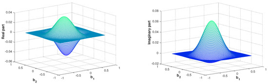
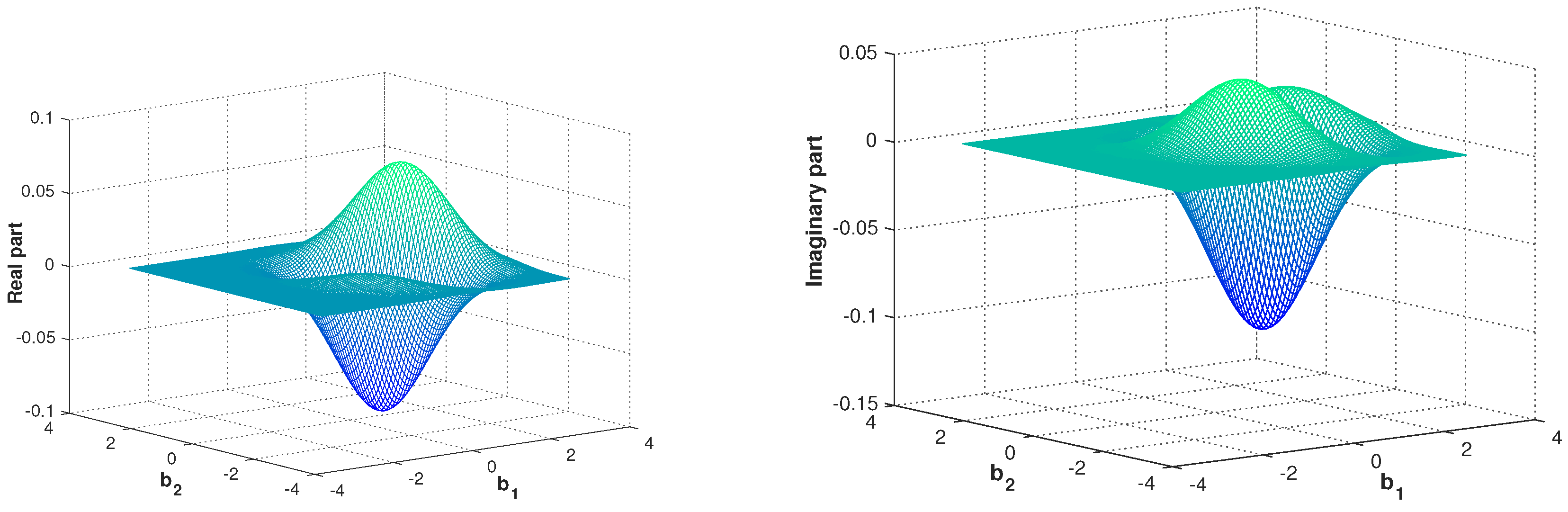
Figure 1. Real and imaginary parts of the non-separable linear canonical wavelet transform of f corresponding to a fixed scale $a=1/4$.

Figure 2. Real and imaginary parts of the non-separable linear canonical wavelet transform of f corresponding to a fixed scale $a=1$.

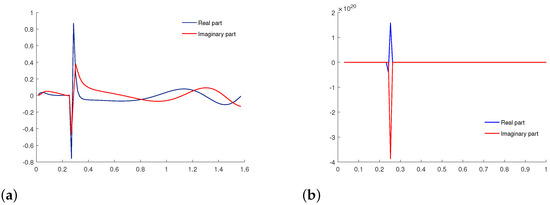
Figure 3. (a) Frequency representation of f corresponding to a position $\mathbf{b}=(0,0)$. (b) Frequency representation of f corresponding to a position $\mathbf{b}=(1,1)$.

(b) Consider the constant function $f\left(\mathbf{t}\right)=K$ and the two-dimensional Morlet wavelet $\psi \left(\mathbf{t}\right)=e^{i\Lambda ·\mathbf{t}-{\left|\mathbf{t}\right|}^2/2},\Lambda =({\lambda }_1,{\lambda }_2)>0$. Then, the non-separable linear canonical wavelet transform of $f\left(\mathbf{t}\right)$ with respect to the real symplectic matrix

$$\begin{array}{c}\hfill \mathbf{M}=\left(\begin{array}{cc}A& B\\ C& D\end{array}\right)=\left(\begin{array}{cccc}2& -1/8& 1/4& -1\\ 1/8& -2& 1& 1/4\\ -2/15& -31/30& 1& 0\\ 1& 2/3& -4/5& -14/15\end{array}\right)\end{array}$$

is given by

$$\begin{array}{cc}\hfill {\mathcal{W}}_{\psi }^{\mathbf{M}}\left[f\right](a,\mathbf{b})& ={\displaystyle \frac{1}{\sqrt{a|detB|}}}exp\left\{{\displaystyle \frac{i\left({\lambda }_1{b}_1+{\lambda }_2{b}_2\right)}{a}}-{\displaystyle \frac{\left(b_1^2+b_2^2\right)}{2a^2}}\right\}\hfill \\ \hfill & \times {\int }_{{\mathbb{R}}^n}Kexp\left\{-{\displaystyle \frac{t_1^2}{2a^2}}+\left({\displaystyle \frac{b_1}{a^2}}-{\displaystyle \frac{i{\lambda }_1}{a}}\right)t_1\right\}exp\left\{-{\displaystyle \frac{t_2^2}{2a^2}}+\left({\displaystyle \frac{b_2}{a^2}}-{\displaystyle \frac{i{\lambda }_2}{a}}\right)t_2\right\}\hfill \\ \hfill & \times exp\left\{-i\pi \left({\Lambda }_a^{T}D{B}^{-1}{\Lambda }_a-2{\Lambda }_a^T{B}^{T^{-1}}\mathbf{t}+{\mathbf{t}}^T{B}^{-1}A\mathbf{t}\right)\right\}d\mathbf{t}.\hfill \end{array}$$

(22)

Moreover, we have

$$\begin{array}{cc}\hfill & {\Lambda }_a^{T}D{B}^{-1}{\Lambda }_a={\displaystyle \frac{16}{15}}\left(\begin{array}{cc}a& a\end{array}\right)\left(\begin{array}{cc}1& 0\\ -4/15& -14/15\end{array}\right)\left(\begin{array}{cc}-1/4& 1\\ -1& 1/4\end{array}\right)\left(\begin{array}{c}a\\ a\end{array}\right)={\displaystyle \frac{12a^2}{25}},\hfill \end{array}$$

(23)

$$\begin{array}{cc}\hfill & {\Lambda }_a^T{B}^{T^{-1}}\mathbf{t}={\displaystyle \frac{16}{15}}\left(\begin{array}{cc}a& a\end{array}\right)\left(\begin{array}{cc}-1/4& 1\\ -1& 1/4\end{array}\right)\left(\begin{array}{c}{t}_1\\ t_2\end{array}\right)=-{\displaystyle \frac{4a}{3}}(t_1-t_2),\hfill \end{array}$$

(24)

$$\begin{array}{cc}\hfill & {\mathbf{t}}^T{B}^{-1}A\mathbf{t}={\displaystyle \frac{16}{15}}\left(\begin{array}{cc}{t}_1& t_2\end{array}\right)\left(\begin{array}{cc}-1/4& 1\\ -1& 1/4\end{array}\right)\left(\begin{array}{cc}2& -1/8\\ 1/8& -2\end{array}\right)\left(\begin{array}{c}{t}_1\\ t_2\end{array}\right)=-{\displaystyle \frac{2}{5}}\left(t_1^2+t_2^2\right).\hfill \end{array}$$

(25)

Implementing Equations (23)–(25) in Equation (22), we obtain

$$\begin{array}{cc}\hfill {\mathcal{W}}_{\psi }^{\mathbf{M}}\left[f\right](a,\mathbf{b})& =K\sqrt{{\displaystyle \frac{15}{16a}}}exp\left\{{\displaystyle \frac{i\left({\lambda }_1{b}_1+{\lambda }_2{b}_2\right)}{a}}-{\displaystyle \frac{\left(b_1^2+b_2^2\right)}{2a^2}}-{\displaystyle \frac{12\pi i{a}^2}{25}}\right\}\hfill \\ \hfill & \times {\int }_{\mathbb{R}}exp\left\{-\left({\displaystyle \frac{1}{2a^2}}-{\displaystyle \frac{2\pi i}{5}}\right)t_1^2+\left({\displaystyle \frac{b_1}{a^2}}-{\displaystyle \frac{i{\lambda }_1}{a}}+{\displaystyle \frac{8a\pi i}{3}}\right)t_1\right\}d{t}_1\hfill \\ \hfill & \times {\int }_{\mathbb{R}}exp\left\{-\left({\displaystyle \frac{1}{2a^2}}-{\displaystyle \frac{2\pi i}{5}}\right)t_2^2+\left({\displaystyle \frac{b_2}{a^2}}-{\displaystyle \frac{i{\lambda }_2}{a}}-{\displaystyle \frac{8a\pi i}{3}}\right)t_2\right\}d{t}_2\hfill \\ \hfill & ={\displaystyle \frac{K\pi }{\left({\displaystyle \frac{1}{2a^2}}-{\displaystyle \frac{2}{5}}\right)}}\sqrt{{\displaystyle \frac{15}{16a}}}exp\left\{{\displaystyle \frac{i\left({\lambda }_1{b}_1+{\lambda }_2{b}_2\right)}{a}}-{\displaystyle \frac{\left(b_1^2+b_2^2\right)}{2a^2}}-{\displaystyle \frac{12\pi i{a}^2}{25}}\right\}\hfill \\ \hfill & \times exp\left\{{\displaystyle \frac{{\left({\displaystyle \frac{b_1}{a^2}}-{\displaystyle \frac{i{\lambda }_1}{a}}+{\displaystyle \frac{8a\pi i}{3}}\right)}^2}{4\left({\displaystyle \frac{1}{2a^2}}-{\displaystyle \frac{2\pi i}{5}}\right)}}\right\}exp\left\{{\displaystyle \frac{{\left({\displaystyle \frac{b_2}{a^2}}-{\displaystyle \frac{i{\lambda }_2}{a}}-{\displaystyle \frac{8a\pi i}{3}}\right)}^2}{4\left({\displaystyle \frac{1}{2a^2}}-{\displaystyle \frac{2\pi i}{5}}\right)}}\right\}.\hfill \end{array}$$

(26)

The non-separable linear canonical wavelet transforms shown in Equation (26) of f corresponding to $\Lambda =(1,1)$ are plotted in Figure 4, Figure 5 and Figure 6.

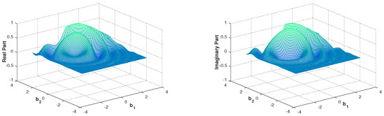
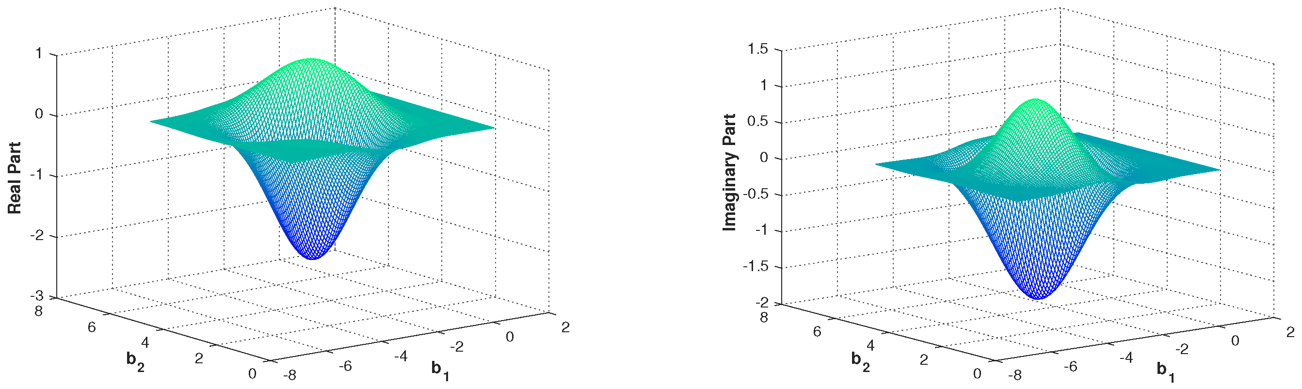
Figure 4. Real and imaginary parts of the non-separable linear canonical wavelet transform of f corresponding to a fixed scale $a=1/4$.

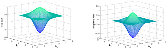
Figure 5. Real and imaginary parts of the non-separable linear canonical wavelet transform of f corresponding to a fixed scale $a=1$.

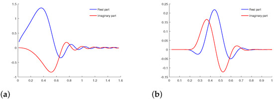
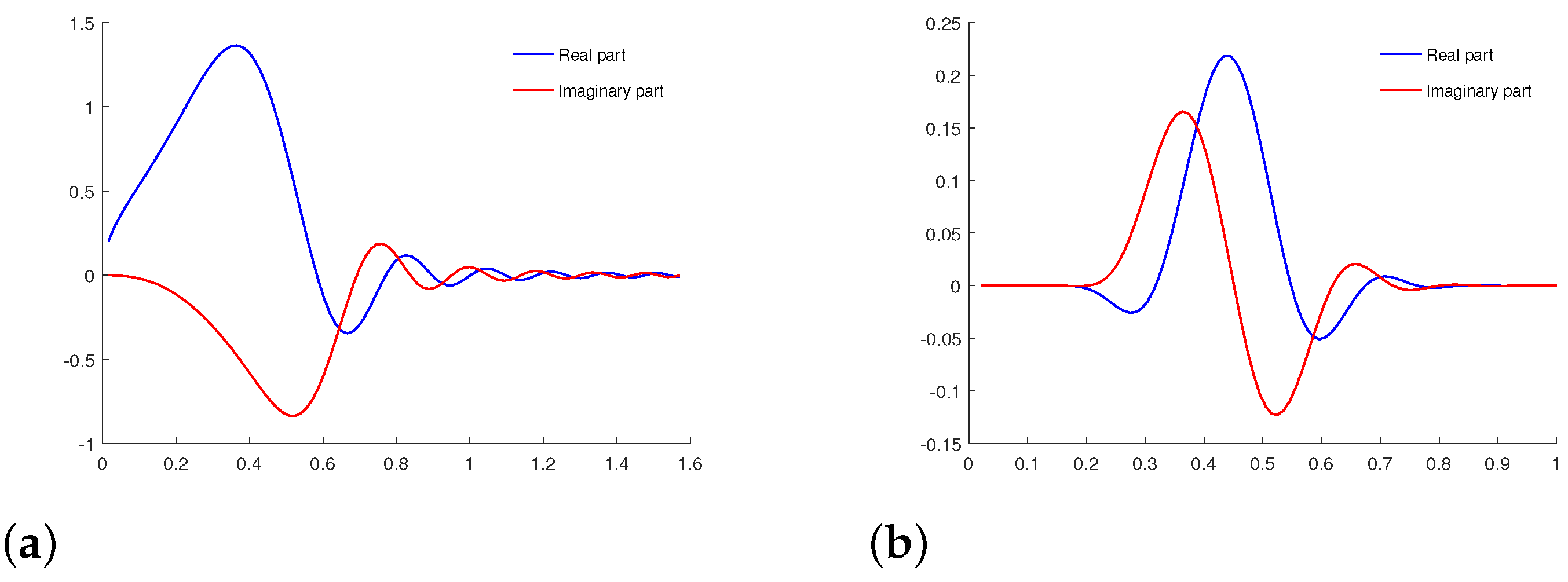
Figure 6. (a) Frequency representation of f corresponding to a position $\mathbf{b}=(0,0)$. (b) Frequency representation of f corresponding to a position $\mathbf{b}=(1,1)$.

Next, we shall derive a fundamental relationship between the non-separable linear canonical wavelet transform (Equation (7)) and the non-separable linear canonical transform (Equation (1)). With the aid of this formula, we shall study the fundamental properties of the proposed transform.

Proposition 1.

Let ${\mathcal{W}}_{\psi }^{\mathbf{M}}\left[f\right](a,\mathbf{b})$ and ${\mathcal{F}}^{\mathbf{M}}\left[f\right]\left(a\right)$ be the non-separable linear canonical wavelet transform and the non-separable linear canonical transform of any $f\in L^2\left({\mathbb{R}}^n\right)$, respectively. Then, we have

$$\begin{array}{c}\hfill {\mathcal{F}}^{\mathbf{M}}\left[{\mathcal{W}}_{\psi }^{\mathbf{M}}\left[f\right]\right]\left(\mathbf{w}\right)=\sqrt{a|detB|}{\mathcal{K}}^{\mathbf{M}}(\mathbf{b},{\Lambda }_a)e^{\pi i{a}^2{\mathbf{w}}^{T}D{B}^{-1}\mathbf{w}}{\mathcal{F}}^{\mathbf{M}}\left[f\right]\left(\mathbf{w}\right)\overline{{\mathcal{F}}^{\mathbf{M}}\left[\Psi \right]\left(a\mathbf{w}\right)},\end{array}$$

(27)

where

$$\begin{array}{c}\hfill \Psi (\mathbf{t},a)=e^{\pi i\left(2{\left(a{\Lambda }_a\right)}^T{B}^{T^{-1}}\mathbf{t}-{\mathbf{t}}^T{B}^{-1}A\mathbf{t}\right)}\psi \left(\mathbf{t}\right).\end{array}$$

(28)

Proof. 

Applying the definition of the non-separable linear canonical transform, we have

$$\begin{array}{cc}\hfill & {\mathcal{F}}^{\mathbf{M}}\left[{\psi }_{a,\mathbf{b}}^{\mathbf{M}}\left(\mathbf{t}\right)\right]\left(\mathbf{w}\right)\hfill \\ \hfill & ={\int }_{{\mathbb{R}}^n}{\displaystyle \frac{1}{\sqrt{a}}}\psi \left({\displaystyle \frac{\mathbf{t}-\mathbf{b}}{a}}\right){\displaystyle \frac{1}{\sqrt{|detB|}}}exp\left\{-\pi i\left({\Lambda }_a^{T}D{B}^{-1}{\Lambda }_a-2{\Lambda }_a^T{B}^{T^{-1}}\mathbf{t}+{\mathbf{t}}^T{B}^{-1}A\mathbf{t}\right)\right\}\hfill \\ \hfill & \times {\displaystyle \frac{1}{\sqrt{|detB|}}}exp\left\{\pi i\left({\mathbf{w}}^{T}D{B}^{-1}\mathbf{w}-2{\mathbf{w}}^T{B}^{T^{-1}}\mathbf{t}+{\mathbf{t}}^T{B}^{-1}A\mathbf{t}\right)\right\}d\mathbf{t}\hfill \\ \hfill & ={\displaystyle \frac{\sqrt{a}}{|detB|}}{\int }_{{\mathbb{R}}^n}\psi \left(\mathbf{z}\right)exp\left\{-\pi i\left({\Lambda }_a^{T}D{B}^{-1}{\Lambda }_a-2{\Lambda }_a^T{B}^{T^{-1}}(\mathbf{b}+a\mathbf{z})\right)\right\}\hfill \\ \hfill & \times exp\left\{\pi i\left({\mathbf{w}}^{T}D{B}^{-1}\mathbf{w}-2{\mathbf{w}}^T{B}^{T^{-1}}(\mathbf{b}+a\mathbf{z})\right)\right\}d\mathbf{z}\hfill \\ \hfill & ={\displaystyle \frac{\sqrt{a}}{|detB|}}{\int }_{{\mathbb{R}}^n}\psi \left(\mathbf{z}\right)exp\left\{\pi i\left({\mathbf{w}}^{T}D{B}^{-1}\mathbf{w}-2\left(a{\mathbf{w}}^T\right)B^{T^{-1}}\mathbf{z}+{\mathbf{z}}^T{B}^{-1}A\mathbf{z}\right)\right\}\hfill \\ \hfill & \times exp\left\{-\pi i\left({\Lambda }_a^{T}D{B}^{-1}{\Lambda }_a-2{\left(a{\Lambda }_a\right)}^T{B}^{T^{-1}}\mathbf{z}+{\mathbf{z}}^T{B}^{-1}A\mathbf{z}\right)\right\}\hfill \\ \hfill & \times exp\left\{\pi i\left(2{\Lambda }_a^T{B}^{T^{-1}}\mathbf{b}-2{\mathbf{w}}^{T}D{B}^{-1}\mathbf{w}\right)\right\}d\mathbf{z}\hfill \\ \hfill & ={\displaystyle \frac{\sqrt{a}}{|detB|}}{\int }_{{\mathbb{R}}^n}\psi \left(\mathbf{z}\right)exp\left\{\pi i\left({\left(a\mathbf{w}\right)}^{T}D{B}^{-1}\left(a\mathbf{w}\right)-2{\left(a\mathbf{w}\right)}^T{B}^{T^{-1}}\mathbf{z}+{\mathbf{z}}^T{B}^{-1}A\mathbf{z}\right)\right\}\hfill \\ \hfill & \times exp\left\{\pi i\left({\mathbf{w}}^{T}D{B}^{-1}\mathbf{w}-2{\mathbf{w}}^T{B}^{T^{-1}}\mathbf{b}+{\mathbf{b}}^T{B}^{-1}A\mathbf{b}\right)\right\}\hfill \\ \hfill & \times exp\left\{-\pi i\left({\Lambda }_a^{T}D{B}^{-1}{\Lambda }_a-2{\Lambda }_a^T{B}^{T^{-1}}\mathbf{b}+{\mathbf{b}}^T{B}^{-1}A\mathbf{b}\right)\right\}\hfill \\ \hfill & \times exp\left\{-\pi i\left({\left(a\mathbf{w}\right)}^{T}D{B}^{-1}\left(a\mathbf{w}\right)-2{\left(a{\Lambda }_a\right)}^T{B}^{T^{-1}}\mathbf{z}+{\mathbf{z}}^T{B}^{-1}A\mathbf{z}\right)\right\}d\mathbf{z}\hfill \\ \hfill & =\sqrt{a|detB|}{e}^{-\pi i{a}^2{\mathbf{w}}^{T}D{B}^{-1}\mathbf{w}}{\mathcal{K}}^{\mathbf{M}}\left(\mathbf{b},\mathbf{w}\right)\overline{{\mathcal{K}}^{\mathbf{M}}(\mathbf{b},{\Lambda }_a)}\hfill \\ \hfill & \times {\int }_{{\mathbb{R}}^n}{e}^{\pi i\left(2{\left(a{\Lambda }_a\right)}^T{B}^{T^{-1}}\mathbf{z}-{\mathbf{z}}^T{B}^{-1}A\mathbf{z}\right)}\psi \left(\mathbf{z}\right){\mathcal{K}}^{\mathbf{M}}(\mathbf{z},a\mathbf{w})d\mathbf{z}\hfill \\ \hfill & =\sqrt{a|detB|}{e}^{-\pi i{a}^2{\mathbf{w}}^{T}D{B}^{-1}\mathbf{w}}{\mathcal{K}}^{\mathbf{M}}\left(\mathbf{b},\mathbf{w}\right)\overline{{\mathcal{K}}^{\mathbf{M}}(\mathbf{b},{\Lambda }_a)}{\mathcal{F}}^{\mathbf{M}}\left[\Psi \right]\left(a\mathbf{w}\right),\hfill \end{array}$$

(29)

where $\Psi (\mathbf{t},a)=e^{\pi i\left(2{\left(a{\Lambda }_a\right)}^T{B}^{T^{-1}}\mathbf{t}-{\mathbf{z}}^T{B}^{-1}A\mathbf{t}\right)}\psi \left(\mathbf{t}\right)$.

Invoking the Plancheral theorem for the non-separable linear canonical transform and using Equation (29), we have

$$\begin{array}{cc}\hfill {\mathcal{W}}_{\psi }^{\mathbf{M}}\left[f\right](a,\mathbf{b})& =\sqrt{a|detB|}{\mathcal{K}}^{\mathbf{M}}(\mathbf{b},{\Lambda }_a){\int }_{{\mathbb{R}}^n}{e}^{\pi i{a}^2{\mathbf{w}}^{T}D{B}^{-1}\mathbf{w}}{\mathcal{F}}^{\mathbf{M}}\left[f\right]\left(\mathbf{w}\right)\overline{{\mathcal{F}}^{\mathbf{M}}\left[\Psi \right]\left(a\mathbf{w}\right)}\overline{{\mathcal{K}}^{\mathbf{M}}\left(\mathbf{b},\mathbf{w}\right)}d\mathbf{w}\hfill \\ \hfill & ={\mathcal{F}}^{{\mathbf{M}}^{-\mathbf{1}}}\left[\sqrt{a|detB|}{\mathcal{K}}^{\mathbf{M}}(\mathbf{b},{\Lambda }_a)e^{\pi i{a}^2{\mathbf{w}}^{T}D{B}^{-1}\mathbf{w}}{\mathcal{F}}^{\mathbf{M}}\left[f\right]\left(\mathbf{w}\right)\overline{{\mathcal{F}}^{\mathbf{M}}\left[\Psi \right]\left(a\mathbf{w}\right)}\right]\left(\mathbf{b}\right).\hfill \end{array}$$

Consequently,

$$\begin{array}{c}\hfill {\mathcal{F}}^{\mathbf{M}}\left[{\mathcal{W}}_{\psi }^{\mathbf{M}}\left[f\right](a,\mathbf{b})\right]\left(\mathbf{w}\right)=\sqrt{a|detB|}{\mathcal{K}}^{\mathbf{M}}(\mathbf{b},{\Lambda }_a)e^{\pi i{a}^2{\mathbf{w}}^{T}D{B}^{-1}\mathbf{w}}{\mathcal{F}}^{\mathbf{M}}\left[f\right]\left(\mathbf{w}\right)\overline{{\mathcal{F}}^{\mathbf{M}}\left[\Psi \right]\left(a\mathbf{w}\right)}.\end{array}$$

This completes the proof of Proposition 1. □

2.3. Basic Properties of the Non-Separable Linear Canonical Wavelet Transform

In this subsection, we shall study some mathematical properties of the proposed non-separable linear canonical wavelet transform (Equation (7)), including Rayleigh’s theorem, inversion formula, and the range theorem. In this direction, we have the following theorem, which assembles some of the basic properties of the proposed transform.

Theorem 1.

For any $f,g\in L^2\left({\mathbb{R}}^n\right)$ and $\alpha ,\beta \in \mathbb{R}$, $\mathbf{k}\in {\mathbb{R}}^n$, and $\mu \in {\mathbb{R}}^{+}$, the non-separable linear canonical wavelet transform as defined by Equation (7) satisfies the following properties:

(i) 

Linearity: ${\mathcal{W}}_{\psi }^{\mathbf{M}}\left[\alpha f+\beta g\right](a,\mathbf{b})=\alpha {\mathcal{W}}_{\psi }^{\mathbf{M}}\left[f\right](a,\mathbf{b})+\beta {\mathcal{W}}_{\psi }^{\mathbf{M}}\left[g\right](a,\mathbf{b})$

(ii) 

Anti-linearity: ${\mathcal{W}}_{\alpha \psi +\beta \varphi }^{\mathbf{M}}\left[,f\right](a,\mathbf{b})=\overline{\alpha }{\mathcal{W}}_{\psi }^{\mathbf{M}}\left[f\right](a,\mathbf{b})+\overline{\beta }{\mathcal{W}}_{\varphi }^{\mathbf{M}}\left[f\right](a,\mathbf{b})$

(iii) 

Translation:

$${\mathcal{W}}_{\psi }^{\mathbf{M}}\left[f(\mathbf{t}-\mathbf{k})\right](a,\mathbf{b})=e^{2\pi i{\Lambda }_a{B}^{T^{-1}}\mathbf{k}}{\mathcal{W}}_{\psi }^{\mathbf{M}}\left[f\left(\mathbf{t}\right)e^{\pi i\left({\mathbf{k}}^T{B}^{-1}A\mathbf{x}+{\mathbf{x}}^T{B}^{-1}A\mathbf{k}\right)}\right](a,\mathbf{b}-\mathbf{k})$$

(iv) 

Scaling: ${\mathcal{W}}_{\psi }^{\mathbf{M}}\left[f\left(\mu \mathbf{t}\right)\right](a,\mathbf{b})={\left|\mu \right|}^{1-\frac{n}{2}}{\mathcal{W}}_{\psi }^{{\mathbf{M}}^{\prime }}f\left(\mu a,\mu \mathbf{b}\right),{\mathbf{M}}^{\prime }=\left(A/\mu ,B/\mu :\mu C,\mu D\right)$

(v) 

Conjugation: ${\mathcal{W}}_{\overline{\psi }}^{\mathbf{M}}\left[\overline{f}\right](a,\mathbf{b})={\displaystyle \frac{1}{\sqrt{a}}}\overline{{\mathcal{W}}_{\psi }^{{\mathbf{M}}^{\prime }}\left[f\right](a,\mathbf{b})},{\mathbf{M}}^{\prime }=\left(A,-B:-C,D\right)$.

Proof. 

For the sake of brevity, we omit the proof of the theorem. □

Next, we shall define the admissibility condition for a function $\psi \in L^2\left({\mathbb{R}}^n\right)$.

Definition 3.

A function $\psi \in L^2\left({\mathbb{R}}^n\right)$ is said to be admissible with respect to a real free symplectic matrix $\mathbf{M}=(A,B:C,D)$ if

$$\begin{array}{c}\hfill C_{\psi }={\int }_{{\mathbb{R}}^{+}}{\displaystyle \frac{|{\mathcal{F}}^{\mathbf{M}}\left[\Psi \right]\left(a\mathbf{w}\right){|}^2}{a}}da<\infty ,a.e.\mathbf{w}\in {\mathbb{R}}^n,\end{array}$$

(30)

where $\Psi (\mathbf{t},a)$ is given by Equation (28).

We are now in a position to derive the orthogonality relation for the proposed transform defined in Equation (7). As a consequence of the orthogonality relation, we will demonstrate that the non-separable wavelet transform is an isometry from the space of square-integrable functions $L^2\left({\mathbb{R}}^n\right)$ to the space of transforms $L^2({\mathbb{R}}^n\times {\mathbb{R}}^{+})$.

Theorem 2.

Let ${\mathcal{W}}_{\psi }^{\mathbf{M}}\left[f\right](a,\mathbf{b})$ and ${\mathcal{W}}_{\psi }^{\mathbf{M}}\left[g\right](a,\mathbf{b})$ be the non-separable linear canonical wavelet transforms of f and g belonging to $L^2\left({\mathbb{R}}^n\right)$, respectively. Then, we have

$$\begin{array}{c}\hfill {\int }_{{\mathbb{R}}^n\times {\mathbb{R}}^{+}}{\mathcal{W}}_{\psi }^{\mathbf{M}}\left[f\right](a,\mathbf{b})\overline{{\mathcal{W}}_{\psi }^{\mathbf{M}}\left[g\right]}(a,\mathbf{b}){\displaystyle \frac{d\mathbf{b}da}{a^2}}=C_{\psi }⟨f,g⟩,\end{array}$$

(31)

where $C_{\psi }$ is given by Equation (30).

Proof. 

For any pair of square integrable functions f and g, Proposition 1 implies that

$$\begin{array}{cc}\hfill {\mathcal{W}}_{\psi }^{\mathbf{M}}\left[f\right](a,\mathbf{b})& =\sqrt{a|detB|}{\int }_{{\mathbb{R}}^n}{e}^{\pi i{a}^2{\mathbf{w}}^{T}D{B}^{-1}\mathbf{w}}{\mathcal{F}}^{\mathbf{M}}\left[f\right]\left(\mathbf{w}\right)\overline{{\mathcal{K}}^{\mathbf{M}}\left(\mathbf{b},\mathbf{w}\right)}{\mathcal{K}}^{\mathbf{M}}(\mathbf{b},{\Lambda }_a)\overline{{\mathcal{F}}^{\mathbf{M}}\left[\Psi \right]\left(a\mathbf{w}\right)}d\mathbf{w}\hfill \end{array}$$

and

$$\begin{array}{cc}\hfill {\mathcal{W}}_{\psi }^{\mathbf{M}}\left[g\right](a,\mathbf{b})& =\sqrt{a|detB|}{\int }_{{\mathbb{R}}^n}{e}^{\pi i{a}^2{\mathbf{x}}^{T}D{B}^{-1}\mathbf{x}}{\mathcal{F}}^{\mathbf{M}}\left[g\right]\left(\mathbf{x}\right)\overline{{\mathcal{K}}^{\mathbf{M}}\left(\mathbf{b},\mathbf{x}\right)}{\mathcal{K}}^{\mathbf{M}}(\mathbf{b},{\Lambda }_a)\overline{{\mathcal{F}}^{\mathbf{M}}\left[\Psi \right]\left(a\mathbf{x}\right)}d\mathbf{x},\hfill \end{array}$$

where $\Psi$ are given by Equation (28). Consequently, we have

$$\begin{array}{cc}\hfill & {\int }_{{\mathbb{R}}^n\times {\mathbb{R}}^{+}}{\mathcal{W}}_{\psi }^{\mathbf{M}}\left[f\right](a,\mathbf{b})\overline{{\mathcal{W}}_{\psi }^{\mathbf{M}}\left[g\right]}(a,\mathbf{b}){\displaystyle \frac{d\mathbf{b}da}{a^2}}\hfill \\ \hfill & =|detB|{\int }_{{\mathbb{R}}^n\times {\mathbb{R}}^n\times {\mathbb{R}}^n\times {\mathbb{R}}^{+}}{e}^{\pi i{a}^2\left({\mathbf{w}}^{T}D{B}^{-1}\mathbf{w}-{\mathbf{x}}^{T}D{B}^{-1}\mathbf{x}\right)}{\mathcal{F}}^{\mathbf{M}}\left[f\right]\left(\mathbf{w}\right)\overline{{\mathcal{F}}^{\mathbf{M}}\left[g\right]\left(\mathbf{x}\right)}\hfill \\ \hfill & \times {\mathcal{F}}^{\mathbf{M}}\left[\Psi \right]\left(a\mathbf{w}\right)\overline{{\mathcal{F}}^{\mathbf{M}}\left[\Psi \right]\left(a\mathbf{x}\right)}{\mathcal{K}}^{\mathbf{M}}(\mathbf{b},{\Lambda }_a)\overline{{\mathcal{K}}^{\mathbf{M}}(\mathbf{b},{\Lambda }_a)}{\mathcal{K}}_{\mathbf{M}}\left(\mathbf{b},\mathbf{x}\right)\overline{{\mathcal{K}}_{\mathbf{M}}\left(\mathbf{b},\mathbf{w}\right)}{\displaystyle \frac{d\mathbf{b}d\mathbf{w}d\mathbf{x}da}{a}}\hfill \\ \hfill & ={\int }_{{\mathbb{R}}^n\times {\mathbb{R}}^n\times {\mathbb{R}}^{+}}{e}^{\pi i{a}^2\left({\mathbf{w}}^{T}D{B}^{-1}\mathbf{w}-{\mathbf{x}}^{T}D{B}^{-1}\mathbf{x}\right)}{\mathcal{F}}^{\mathbf{M}}\left[f\right]\left(\mathbf{w}\right)\overline{{\mathcal{F}}^{\mathbf{M}}\left[g\right]\left(\mathbf{x}\right)}\hfill \\ \hfill & \times {\mathcal{F}}^{\mathbf{M}}\left[\Psi \right]\left(a\mathbf{w}\right)\overline{{\mathcal{F}}^{\mathbf{M}}\left[\Psi \right]\left(a\mathbf{x}\right)}\left\{{\int }_{{\mathbb{R}}^n}{\mathcal{K}}_{\mathbf{M}}\left(\mathbf{b},\mathbf{x}\right)\overline{{\mathcal{K}}_{\mathbf{M}}\left(\mathbf{b},\mathbf{w}\right)}d\mathbf{b}\right\}{\displaystyle \frac{d\mathbf{w}d\mathbf{x}da}{a}}\hfill \\ \hfill & ={\int }_{{\mathbb{R}}^n\times {\mathbb{R}}^n\times {\mathbb{R}}^{+}}{e}^{\pi i{a}^2\left({\mathbf{w}}^{T}D{B}^{-1}\mathbf{w}-{\mathbf{x}}^{T}D{B}^{-1}\mathbf{x}\right)}{\mathcal{F}}^{\mathbf{M}}\left[f\right]\left(\mathbf{w}\right)\overline{{\mathcal{F}}^{\mathbf{M}}\left[g\right]\left(\mathbf{v}\right)}\hfill \\ \hfill & \times {\mathcal{F}}^{\mathbf{M}}\left[\Psi \right]\left(a\mathbf{w}\right)\overline{{\mathcal{F}}^{\mathbf{M}}\left[\Psi \right]\left(a\mathbf{x}\right)}\delta \left(\mathbf{w}-\mathbf{x}\right){\displaystyle \frac{d\mathbf{w}d\mathbf{x}da}{a}}\hfill \\ \hfill & ={\int }_{{\mathbb{R}}^n\times {\mathbb{R}}^{+}}{\mathcal{F}}^{\mathbf{M}}\left[f\right]\left(\mathbf{w}\right)\overline{{\mathcal{F}}^{\mathbf{M}}\left[g\right]\left(\mathbf{w}\right)}{\left|{\mathcal{F}}^{\mathbf{M}}\left[\Psi \right]\left(a\mathbf{w}\right)\right|}^2{\displaystyle \frac{d\mathbf{w}da}{a}}\hfill \\ \hfill & ={\int }_{{\mathbb{R}}^n}{\mathcal{F}}^{\mathbf{M}}\left[f\right]\left(\mathbf{w}\right)\overline{{\mathcal{F}}^{\mathbf{M}}\left[g\right]\left(\mathbf{w}\right)}\left\{{\int }_{{\mathbb{R}}^{+}}{\displaystyle \frac{{\left|{\mathcal{F}}^{\mathbf{M}}\left[\Psi \right]\left(a\mathbf{w}\right)\right|}^2}{a}}da\right\}d\mathbf{w}\hfill \\ \hfill & =C_{\psi }{⟨{\mathcal{F}}^{\mathbf{M}}\left[f\right]\left(\mathbf{w}\right),{\mathcal{F}}^{\mathbf{M}}\left[g\right]\left(\mathbf{w}\right)⟩}_2\hfill \\ \hfill & =C_{\psi }{⟨f,g⟩}_2.\hfill \end{array}$$

This completes the proof of Theorem 2. □

Remark 1.  (i). For $f=g$, Theorem 2 yields the energy preserving relation associated with the non-separable linear canonical wavelet transform (Equation (10)):

$$\begin{array}{c}\hfill {\int }_{{\mathbb{R}}^n\times {\mathbb{R}}^{+}}{\left|{\mathcal{W}}_{\psi }^{\mathbf{M}}\left[f\right](a,\mathbf{b})\right|}^2{\displaystyle \frac{d\mathbf{b}da}{a^2}}=C_{\psi }\parallel f{\parallel }_2^2.\end{array}$$

(32)

(ii). The operator ${\mathcal{W}}_{\psi }^{\mathbf{M}}$ is a bounded-linear operator. Moreover, for $C_{\psi }=1$ and $|detB|=1$, the operator ${\mathcal{W}}_{\psi }^{\mathbf{M}}$ becomes an isometry from $L^2\left({\mathbb{R}}^n\right)$ to $L^2({\mathbb{R}}^n\times {\mathbb{R}}^{+})$.

In our next theorem, we demonstrate that the non-separable linear canonical wavelet transform ${\mathcal{W}}_{\psi }^{\mathbf{M}}\left[f\right](a,\mathbf{b})$ of any function $f\in L^2\left({\mathbb{R}}^n\right)$ is reversible in the sense that f can be easily recovered from the transformed domain $L^2({\mathbb{R}}^n\times {\mathbb{R}}^{+})$.

Theorem 3.

Let ${\mathcal{W}}_{\psi }^{\mathbf{M}}\left[f\right](a,\mathbf{b})$ be the non-separable linear canonical wavelet transform of an arbitrary function $f\in L^2\left({\mathbb{R}}^n\right)$. Then, f can be reconstructed via

$$\begin{array}{c}\hfill f\left(\mathbf{t}\right)={\displaystyle \frac{1}{C_{\psi }}}{\int }_{{\mathbb{R}}^n\times {\mathbb{R}}^{+}}{\mathcal{W}}_{\psi }^{\mathbf{M}}\left[f\right](a,\mathbf{b}){\psi }_{a,\mathbf{b}}^{\mathbf{M}}\left(\mathbf{t}\right){\displaystyle \frac{d\mathbf{b}da}{a^2}},a.e.\end{array}$$

(33)

Proof. 

According to Theorem 2, we can write

$$\begin{array}{cc}\hfill ⟨f,g⟩& ={\displaystyle \frac{1}{C_{\psi }}}{\int }_{{\mathbb{R}}^n\times {\mathbb{R}}^{+}}{\mathcal{W}}_{\psi }^{\mathbf{M}}\left[f\right](a,\mathbf{b})\overline{{\mathcal{W}}_{\psi }^{\mathbf{M}}\left[g\right]}(a,\mathbf{b}){\displaystyle \frac{d\mathbf{b}da}{a^2}}\hfill \\ \hfill & ={\displaystyle \frac{1}{C_{\psi }}}{\int }_{{\mathbb{R}}^n\times {\mathbb{R}}^{+}}{\mathcal{W}}_{\psi }^{\mathbf{M}}\left[f\right](a,\mathbf{b})\left\{{\int }_{{\mathbb{R}}^n}\overline{g\left(\mathbf{t}\right)}{\psi }_{a,\mathbf{b}}^{\mathbf{M}}\left(\mathbf{t}\right)d\mathbf{t}\right\}{\displaystyle \frac{d\mathbf{b}da}{a^2}}\hfill \\ \hfill & ={\displaystyle \frac{1}{C_{\psi }}}{\int }_{{\mathbb{R}}^n\times {\mathbb{R}}^n\times {\mathbb{R}}^{+}}{\mathcal{W}}_{\psi }^{\mathbf{M}}\left[f\right](a,\mathbf{b}){\psi }_{a,\mathbf{b}}^{\mathbf{M}}\left(\mathbf{t}\right)\overline{g\left(\mathbf{t}\right)}{\displaystyle \frac{d\mathbf{t}d\mathbf{b}da}{a^2}}\hfill \\ \hfill & ={\displaystyle \frac{1}{C_{\psi }}}⟨{\int }_{{\mathbb{R}}^n\times {\mathbb{R}}^{+}}{\mathcal{W}}_{\psi }^{\mathbf{M}}\left[f\right](a,\mathbf{b}){\psi }_{a,\mathbf{b}}^{\mathbf{M}}\left(\mathbf{t}\right){\displaystyle \frac{d\mathbf{b}da}{a^2}},g\left(\mathbf{t}\right)⟩.\hfill \end{array}$$

Since g is chosen arbitrarily from $L^2\left({\mathbb{R}}^n\right)$, using the elementary properties of inner products, one can obtain

$$\begin{array}{c}\hfill f\left(\mathbf{t}\right)={\displaystyle \frac{1}{C_{\psi }}}{\int }_{{\mathbb{R}}^n\times {\mathbb{R}}^{+}}{\mathcal{W}}_{\psi }^{\mathbf{M}}\left[f\right](a,\mathbf{b}){\psi }_{a,\mathbf{b}}^{\mathbf{M}}\left(\mathbf{t}\right){\displaystyle \frac{d\mathbf{b}da}{a^2}}a.e.\end{array}$$

This completes the proof of Theorem 3. □

Finally, we investigate the characterization of the range for the proposed transform (Equation (7)). As a consequence of the range theorem, we shall demonstrate that the range of the non-separable linear canonical wavelet transforms; that is, ${\mathcal{W}}_{\psi }^{\mathbf{M}}\left(L^2\left({\mathbb{R}}^n\right)\right)$ is a reproducing kernel Hilbert space.

Theorem 4.

If $f\in L^2({\mathbb{R}}^n\times {\mathbb{R}}^{+})$, then f belongs to the range ${\mathcal{W}}_{\psi }^{\mathbf{M}}\left(L^2\left({\mathbb{R}}^n\right)\right)$ if and only if

$$\begin{array}{c}\hfill f\left(a^{\prime },{\mathbf{b}}^{\prime }\right)={\displaystyle \frac{1}{C_{\psi }}}{\int }_{{\mathbb{R}}^n\times {\mathbb{R}}^{+}}f(a,\mathbf{b}){⟨{\psi }_{a,\mathbf{b}}^{\mathbf{M}},{\psi }_{a^{\prime },{\mathbf{b}}^{\prime }}^{\mathbf{M}}⟩}_2{\displaystyle \frac{d\mathbf{b}da}{a^2}},\end{array}$$

(34)

where $C_{\psi }$ satisfies Equation (27).

Proof. 

Assume that $f\in {\mathcal{W}}_{\psi }^{\mathbf{M}}\left(L^2\left({\mathbb{R}}^n\right)\right)$. Then, there exists a square integrable function g such that ${\mathcal{W}}_{\psi }^{\mathbf{M}}g=f$. In order to show that f satisfies Equation (34), we proceed as

$$\begin{array}{cc}\hfill f\left(a^{\prime },{\mathbf{b}}^{\prime }\right)& ={\mathcal{W}}_{\psi }^{\mathbf{M}}\left[g\right]\left(a^{\prime },{\mathbf{b}}^{\prime }\right)\hfill \\ \hfill & ={\int }_{{\mathbb{R}}^n}g\left(\mathbf{t}\right)\overline{{\psi }_{a^{\prime },{\mathbf{b}}^{\prime }}^{\mathbf{M}}}\left(\mathbf{t}\right)d\mathbf{t}\hfill \\ \hfill & ={\displaystyle \frac{1}{C_{\psi }}}{\int }_{{\mathbb{R}}^n}\left\{{\int }_{{\mathbb{R}}^n\times {\mathbb{R}}^{+}}{\mathcal{W}}_{\psi }^{\mathbf{M}}\left[g\right](a,\mathbf{b}){\psi }_{a,\mathbf{b}}^{\mathbf{M}}\left(\mathbf{t}\right){\displaystyle \frac{d\mathbf{b}da}{a^2}}\right\}\overline{{\psi }_{a^{\prime },{\mathbf{b}}^{\prime }}^{\mathbf{M}}}\left(\mathbf{t}\right)d\mathbf{t}\hfill \\ \hfill & ={\displaystyle \frac{1}{C_{\psi }}}{\int }_{{\mathbb{R}}^n\times {\mathbb{R}}^{+}}{\mathcal{W}}_{\psi }^{\mathbf{M}}\left[g\right](a,\mathbf{b})\left\{{\int }_{\mathbb{R}}{\psi }_{a,\mathbf{b}}^{\mathbf{M}}\left(\mathbf{t}\right)\overline{{\psi }_{a^{\prime },{\mathbf{b}}^{\prime }}^{\mathbf{M}}}\left(\mathbf{t}\right)d\mathbf{t}\right\}{\displaystyle \frac{d\mathbf{b}da}{a^2}}\hfill \\ \hfill & ={\displaystyle \frac{1}{C_{\psi }}}{\int }_{{\mathbb{R}}^n\times {\mathbb{R}}^{+}}f(a,\mathbf{b}){⟨{\psi }_{a,\mathbf{b}}^{\mathbf{M}},{\psi }_{a^{\prime },{\mathbf{b}}^{\prime }}^{\mathbf{M}}⟩}_2{\displaystyle \frac{d\mathbf{b}da}{a^2}},\hfill \end{array}$$

which evidently verifies our claim. Conversely, suppose that the function f satisfies Equation (34). To verify that $f\in {\mathcal{W}}_{\psi }^{\mathbf{M}}\left(L^2\left({\mathbb{R}}^n\right)\right)$, it is sufficient to find out a function $g\in L^2\left({\mathbb{R}}^n\right)$ such that ${\mathcal{W}}_{\psi }^{\mathbf{M}}g=f$. Therefore, the desired function g will be constructed as follows:

Let

$$\begin{array}{c}\hfill g\left(\mathbf{t}\right)={\displaystyle \frac{1}{C_{\psi }}}{\int }_{{\mathbb{R}}^n\times {\mathbb{R}}^{+}}f(a,\mathbf{b}){\psi }_{a,\mathbf{b}}^{\mathbf{M}}\left(\mathbf{t}\right){\displaystyle \frac{d\mathbf{b}da}{a^2}}.\end{array}$$

(35)

Then, it is straightforward to obtain $\parallel g{\parallel }_2\le \parallel f{\parallel }_2<\infty$; that is $g\in L^2\left({\mathbb{R}}^n\right)$. Furthermore, by virtue of the Fubini theorem, we have

$$\begin{array}{cc}\hfill {\mathcal{W}}_{\psi }^{\mathbf{M}}\left[g\right]\left(a^{\prime },{\mathbf{b}}^{\prime }\right)& ={\int }_{{\mathbb{R}}^n}g\left(\mathbf{x}\right)\overline{{\psi }_{a^{\prime },{\mathbf{b}}^{\prime }}^{\mathbf{M}}}\left(\mathbf{t}\right)d\mathbf{t}\hfill \\ \hfill & ={\displaystyle \frac{1}{C_{\psi }}}{\int }_{{\mathbb{R}}^n}\left\{{\int }_{{\mathbb{R}}^n\times {\mathbb{R}}^{+}}f(a,\mathbf{b}){\psi }_{a,\mathbf{b}}^{\mathbf{M}}\left(\mathbf{t}\right){\displaystyle \frac{d\mathbf{b}da}{a^2}}\right\}\overline{{\psi }_{a^{\prime },{\mathbf{b}}^{\prime }}^{\mathbf{M}}}\left(\mathbf{t}\right)d\mathbf{t}\hfill \\ \hfill & ={\displaystyle \frac{1}{C_{\psi }}}{\int }_{{\mathbb{R}}^n\times {\mathbb{R}}^{+}}f(a,\mathbf{b}){⟨{\psi }_{a,\mathbf{b}}^{\mathbf{M}},{\psi }_{a^{\prime },{\mathbf{b}}^{\prime }}^{\mathbf{M}}⟩}_2{\displaystyle \frac{d\mathbf{b}da}{a^2}}\hfill \\ \hfill & =f\left(a^{\prime },{\mathbf{b}}^{\prime }\right).\hfill \end{array}$$

This completes the proof of Theorem 4. □

Corollary 1.

For any admissible wavelet $\psi \in L^2\left({\mathbb{R}}^n\right)$, the range of the proposed non-separable linear canonical wavelet transform; that is, ${\mathcal{W}}_{\psi }^{\mathbf{M}}\left(L^2\left({\mathbb{R}}^n\right)\right)$ is a reproducing kernel Hilbert space embedded as a subspace in $L^2\left({\mathbb{R}}^n\times {\mathbb{R}}^{+}\right)$ with the kernel given by

$$\begin{array}{c}\hfill K_{\psi }^{\Lambda }\left(a,\mathbf{b};a^{\prime },{\mathbf{b}}^{\prime }\right)={⟨{\psi }_{a,\mathbf{b}}^{\mathbf{M}},{\psi }_{a^{\prime },{\mathbf{b}}^{\prime }}^{\mathbf{M}}⟩}_2.\end{array}$$

(36)

3. Uncertainty Principles for the Non-Separable Linear Canonical Wavelet Transform

The uncertainty principle lies at the heart of harmonic analysis, which asserts that “the position and the velocity of a particle cannot be both determined precisely at the same time” [23]. The harmonic analysis version of this principle states that “a non-trivial function cannot be properly localized in both the time and frequency domains at the same time” [24]. This standard inequality has been extensively studied in numerous domains and vistas [25,26,27]. Keeping in view the fact that the theory of uncertainty principles for the non-separable linear canonical wavelet transform is yet to be explored exclusively; therefore, it is both theoretically and practically fascinating to develop some new uncertainty principles, including the Heisenberg’s, logarithmic, and Nazaros uncertainty principles for the non-separable linear canonical wavelet transform 7.

Theorem 5.

Let ${\mathcal{W}}_{\psi }^{\mathbf{M}}\left[f\right](a,\mathbf{b})$ be the non-separable linear canonical wavelet transform of any non-trivial function $f\in L^2\left({\mathbb{R}}^n\right)$ with respect to a real free symplectic matrix $\mathbf{M}=(A,B:C,D)$, then the following uncertainty inequality holds:

$$\begin{array}{c}\hfill {\left\{{\int }_{{\mathbb{R}}^n\times {\mathbb{R}}^{+}}|\mathbf{b}{|}^2{\left|{\mathcal{W}}_{\psi }^{\mathbf{M}}\left[f\right](a,\mathbf{b})\right|}^2{\displaystyle \frac{dad\mathbf{b}}{a^2}}\right\}}^{1/2}{\left\{{\int }_{{\mathbb{R}}^n}|\mathbf{w}{|}^2\left|{\mathcal{F}}^{\mathbf{M}}\left[f\right]\left(\mathbf{w}\right)\right|d\mathbf{w}\right\}}^{1/2}\ge {\displaystyle \frac{n{\sigma }_{min}\left(B\right)\sqrt{C_{\psi }}}{4\pi }}\parallel f{\parallel }_2^2,\end{array}$$

(37)

where ${\sigma }_{min}\left(B\right)$ denotes the minimum singular value of matrix B.

Proof. 

The classical Heisenberg–Pauli–Weyl uncertainty inequality for any $f\in L^2\left({\mathbb{R}}^n\right)$ in the non-separable linear canonical domain is given by [7]:

$$\begin{array}{c}\hfill {\left\{{\int }_{{\mathbb{R}}^n}\left|\mathbf{b}{|}^2\right|f\left(\mathbf{b}\right){|}^{2}d\mathbf{b}\right\}}^{1/2}{\left\{{\int }_{{\mathbb{R}}^n}|\mathbf{w}{|}^2{\left|{\mathcal{F}}^{\mathbf{M}}\left[f\right]\left(\mathbf{w}\right)\right|}^{2}d\mathbf{w}\right\}}^{1/2}\ge {\displaystyle \frac{n{\sigma }_{min}\left(B\right)}{4\pi }}\left\{{\int }_{{\mathbb{R}}^n}|f\left(\mathbf{b}\right){|}^{2}d\mathbf{b}\right\}.\end{array}$$

(38)

We shall identify ${\mathcal{W}}_{\psi }^{\mathbf{M}}\left[f\right](a,\mathbf{b})$ as a function of the time variable $\mathbf{b}$ and then invoke Equation (38) so that

$$\begin{array}{c}\hfill {\left\{{\int }_{{\mathbb{R}}^n}\left|\mathbf{b}{|}^2\right|{\mathcal{W}}_{\psi }^{\mathbf{M}}\left[f\right](a,\mathbf{b}){|}^{2}d\mathbf{b}\right\}}^{1/2}{\left\{{\int }_{{\mathbb{R}}^n}|\mathbf{w}{|}^2{\left|{\mathcal{F}}^{\mathbf{M}}\left[{\mathcal{W}}_{\psi }^{\mathbf{M}}\left[f\right](a,\mathbf{b})\right]\left(\mathbf{w}\right)\right|}^{2}d\mathbf{w}\right\}}^{1/2}\\ \hfill \ge {\displaystyle \frac{n{\sigma }_{min}\left(B\right)}{4\pi }}\left\{{\int }_{{\mathbb{R}}^n}{\left|{\mathcal{W}}_{\psi }^{\mathbf{M}}\left[f\right](a,\mathbf{b})\right|}^{2}d\mathbf{b}\right\}.\end{array}$$

(39)

Integrating Equation (39) with respect to the $da/a^2$, we obtain

$$\begin{array}{c}\hfill {\int }_{{\mathbb{R}}^{+}}{\left\{{\int }_{{\mathbb{R}}^n}|\mathbf{b}{|}^2{\left|{\mathcal{W}}_{\psi }^{\mathbf{M}}\left[f\right](a,\mathbf{b})\right|}^{2}d\mathbf{b}\right\}}^{1/2}{\left\{{\int }_{{\mathbb{R}}^n}|\mathbf{w}{|}^2{\left|{\mathcal{F}}^{\mathbf{M}}\left[{\mathcal{W}}_{\psi }^{\mathbf{M}}\left[f\right](a,\mathbf{b})\right]\left(\mathbf{w}\right)\right|}^{2}d\mathbf{w}\right\}}^{1/2}{\displaystyle \frac{da}{a^2}}\\ \hfill \ge {\displaystyle \frac{n{\sigma }_{min}\left(B\right)}{4\pi }}\left\{{\int }_{{\mathbb{R}}^n\times {\mathbb{R}}^{+}}{\left|{\mathcal{W}}_{\psi }^{\mathbf{M}}\left[f\right](a,\mathbf{b})\right|}^2{\displaystyle \frac{d\mathbf{b}da}{a^2}}\right\}.\end{array}$$

(40)

As a consequence of the Cauchy–Schwartz’s inequality, Fubini theorem, and Equation (30), we can express Equation (40) as

$$\begin{array}{c}\hfill {\left\{{\int }_{{\mathbb{R}}^n\times {\mathbb{R}}^{+}}|\mathbf{b}{|}^2{\left|{\mathcal{W}}_{\psi }^{\mathbf{M}}\left[f\right](a,\mathbf{b})\right|}^2{\displaystyle \frac{dad\mathbf{b}}{a^2}}\right\}}^{1/2}{\left\{{\int }_{{\mathbb{R}}^n\times {\mathbb{R}}^{+}}|\mathbf{w}{|}^2{\left|{\mathcal{F}}^{\mathbf{M}}\left[{\mathcal{W}}_{\psi }^{\mathbf{M}}\left[f\right](a,\mathbf{b})\right]\left(\mathbf{w}\right)\right|}^2{\displaystyle \frac{d\mathbf{w}da}{a^2}}\right\}}^{1/2}\\ \hfill \ge {\displaystyle \frac{n{\sigma }_{min}\left(B\right)C_{\psi }}{4\pi }}\parallel f{\parallel }_2^2.\end{array}$$

Using Proposition 1, we can rewrite the above inequality as follows

$$\begin{array}{c}\hfill {\left\{{\int }_{{\mathbb{R}}^n\times {\mathbb{R}}^{+}}|\mathbf{b}{|}^2{\left|{\mathcal{W}}_{\psi }^{\mathbf{M}}\left[f\right](a,\mathbf{b})\right|}^2{\displaystyle \frac{dad\mathbf{b}}{a^2}}\right\}}^{1/2}{\left\{{\int }_{{\mathbb{R}}^n\times {\mathbb{R}}^{+}}\left|\mathbf{w}{|}^2\right|{\mathcal{F}}^{\mathbf{M}}\left[f\right]\left(\mathbf{w}\right){\mathcal{F}}^{\mathbf{M}}\left[\Psi \right]\left(a\mathbf{w}\right){|}^2{\displaystyle \frac{dad\mathbf{w}}{a}}\right\}}^{1/2}\\ \hfill \ge {\displaystyle \frac{n{\sigma }_{min}\left(B\right)C_{\psi }}{4\pi }}\parallel f{\parallel }_2^2,\end{array}$$

or equivalently,

$$\begin{array}{c}\hfill {\left\{{\int }_{{\mathbb{R}}^n\times {\mathbb{R}}^{+}}|\mathbf{b}{|}^2{\left|{\mathcal{W}}_{\psi }^{\mathbf{M}}\left[f\right](a,\mathbf{b})\right|}^2{\displaystyle \frac{dad\mathbf{b}}{a^2}}\right\}}^{1/2}{\left\{{\int }_{{\mathbb{R}}^n}|\mathbf{w}{|}^2{\left|{\mathcal{F}}^{\mathbf{M}}\left[f\right]\left(\mathbf{w}\right)\right|}^2\left({\int }_{{\mathbb{R}}^{+}}{\displaystyle \frac{{\left|{\mathcal{F}}^{\mathbf{M}}\left[\Psi \right]\left(\mathbf{a}\mathbf{w}\right)\right|}^2}{a}}da\right)d\mathbf{w}\right\}}^{1/2}\\ \hfill \ge {\displaystyle \frac{n{\sigma }_{min}\left(B\right)C_{\psi }}{4\pi }}\parallel f{\parallel }_2^2.\end{array}$$

Finally, using Equation (27), we obtain the desired result:

$$\begin{array}{c}\hfill {\left\{{\int }_{{\mathbb{R}}^n\times {\mathbb{R}}^{+}}|\mathbf{b}{|}^2{\left|{\mathcal{W}}_{\psi }^{\mathbf{M}}\left[f\right](a,\mathbf{b})\right|}^2{\displaystyle \frac{dad\mathbf{b}}{a^2}}\right\}}^{1/2}{\left\{{\int }_{{\mathbb{R}}^n}|\mathbf{w}{|}^2\left|{\mathcal{F}}^{\mathbf{M}}\left[f\right]\left(\mathbf{w}\right)\right|d\mathbf{w}\right\}}^{1/2}\ge {\displaystyle \frac{n{\sigma }_{min}\left(B\right)\sqrt{C_{\psi }}}{4\pi }}\parallel f{\parallel }_2^2.\end{array}$$

This completes the proof of Theorem 5. □

Remark 2.

The uncertainty inequality in Equation (37) embodies a wide class of uncertainty relations including the ones corresponding to the separable linear canonical wavelet transform, fractional wavelet transform, and classical wavelet transforms. The corresponding uncertainty principles can be obtained by choosing an appropriate matrix parameter $\mathbf{M}=(A,B:C,D)$.

Example 2.

For the sake of computational convenience, we restrict ourselves to the two-dimensional space. From the inequality in Equation (37), we observe that the lower bound can be adjusted suitably by choosing a real, free symplectic matrix $\mathbf{M}=(A,B:C,D)$ and the analyzing function ψ.

(i).Consider the real, free symplectic matrix

$$\begin{array}{c}\hfill {\mathbf{M}}_1=\left(\begin{array}{cc}{A}_1& B_1\\ C_1& D_1\end{array}\right)=\left(\begin{array}{cccc}1/2& -3/2& 1& -1\\ 3/2& 1/2& -1& -1\\ 0& -1& 1& -1\\ -1& 0& 1& 1\end{array}\right)\end{array}$$

and the two-dimensional Morlet wavelet ${\psi }_1\left(\mathbf{t}\right)$ given by

$${\psi }_1\left(\mathbf{t}\right)=e^{i\Lambda ·\mathbf{t}-{\left|\mathbf{t}\right|}^2/2},\Lambda =({\lambda }_1,{\lambda }_2)>0.$$

Then, by virtue of Equation (28), we obtain

$$\begin{array}{cc}\hfill \Psi (\mathbf{t},a)& =exp\left\{\pi i\left(2a{\Lambda }_a^T{B}^{T^{-1}}\mathbf{t}-{\mathbf{t}}^T{B}^{-1}A\mathbf{t}\right)\right\}\psi \left(\mathbf{t}\right)\hfill \\ \hfill & =exp\left\{\pi i\left(-2a^2{t}_2+{\displaystyle \frac{t_1^2+t_2^2}{2}}\right)\right\}exp\left\{i({\lambda }_1{t}_1+{\lambda }_2{t}_2)-{\displaystyle \frac{t_1^2+t_2^2}{2}}\right\}\hfill \\ \hfill & =exp\left\{-\left({\displaystyle \frac{1-\pi i}{2}}\right)t_1^2+{\lambda }_1{t}_1\right\}exp\left\{-\left({\displaystyle \frac{1-\pi i}{2}}\right)t_2^2+({\lambda }_2-2a^2)t_2\right\}.\hfill \end{array}$$

Subsequently, we have

$$\begin{array}{cc}\hfill & {\mathcal{F}}^{\mathbf{M}}\left[\Psi \right]\left(a\mathbf{w}\right)\hfill \\ \hfill & ={\displaystyle \frac{1}{{|detB|}^{1/2}}}{\int }_{{\mathbb{R}}^2}\Psi (\mathbf{t},a)exp\left\{\pi i\left({\left(a\mathbf{w}\right)}^{T}D{B}^{-1}\left(a\mathbf{w}\right)-2{\left(a\mathbf{w}\right)}^T{B}^{T^{-1}}\mathbf{t}+{\mathbf{t}}^T{B}^{-1}A\mathbf{t}\right)\right\}d\mathbf{t}\hfill \\ \hfill & ={\displaystyle \frac{1}{{|detB|}^{1/2}}}{\int }_{{\mathbb{R}}^2}exp\left\{-\left({\displaystyle \frac{1-\pi i}{2}}\right)t_1^2+{\lambda }_1{t}_1\right\}exp\left\{-\left({\displaystyle \frac{1-\pi i}{2}}\right)t_2^2+({\lambda }_2-2a^2)t_2\right\}\hfill \\ \hfill & \times exp\left\{\pi i\left(a^2\left({\omega }_1^2-{\omega }_2^2\right)+a{\omega }_1(t_2-t_1)+a{\omega }_2(t_1+t_2)-{\displaystyle \frac{t_1^2+t_2^2}{2}}\right)\right\}d{t}_{1}d{t}_2\hfill \\ \hfill & =\sqrt{2}{e}^{\pi i{a}^2\left({\omega }_1^2-{\omega }_2^2\right)}{\int }_{\mathbb{R}}exp\left\{-{\displaystyle \frac{t_1^2}{2}}+\left({\lambda }_1-a\pi i({\omega }_1-{\omega }_2)\right)t_1\right\}d{t}_1\hfill \\ \hfill & \times {\int }_{\mathbb{R}}exp\left\{-{\displaystyle \frac{t_2^2}{2}}+\left({\lambda }_2-2a^2+a\pi i({\omega }_1+{\omega }_2)\right)t_1\right\}d{t}_2\hfill \\ \hfill & =2\pi \sqrt{2a}{e}^{\pi i{a}^2\left({\omega }_1^2-{\omega }_2^2\right)}exp\left\{{\displaystyle \frac{{\left({\lambda }_1-a\pi i({\omega }_1-{\omega }_2)\right)}^2}{2}}\right\}exp\left\{{\displaystyle \frac{{\left({\lambda }_2-2a^2+a\pi i({\omega }_1+{\omega }_2)\right)}^2}{2}}\right\}.\hfill \end{array}$$

Taking ${\lambda }_1=a\pi i$ and ${\lambda }_2=2a^2$, we obtain

$$\begin{array}{c}\hfill {\left|{\mathcal{F}}^{\mathbf{M}}\left[\Psi \right]\left(a\mathbf{w}\right)\right|}^2=8{\pi }^{2}aexp\left\{-a^2{\pi }^2\left(1+2{\omega }_1^2+2{\omega }_2^2+{\omega }_2\right)\right\}.\end{array}$$

(41)

Implementing Equation (41) in Equation (30) yields

$$\begin{array}{cc}\hfill C_{\psi }& =8{\pi }^2{\int }_{{\mathbb{R}}^{+}}exp\left\{-{\pi }^2\left(1+2{\omega }_1^2+2{\omega }_2^2+{\omega }_2\right)a^2\right\}da={\displaystyle \frac{4{\pi }^{3/2}}{\sqrt{1+2{\omega }_1^2+2{\omega }_2^2+{\omega }_2}}}.\hfill \end{array}$$

In particular, for $({\omega }_1,{\omega }_2)=(1,1)$, we obtain

$$\begin{array}{c}\hfill C_{\psi }={\displaystyle \frac{4{\pi }^{3/2}}{\sqrt{6}}}.\end{array}$$

(42)

Therefore, for any normalized function $f\in L^2\left({\mathbb{R}}^2\right)$, an application of Equation (42) in Equation (37) yields the lower bound for the Heisenberg’s inequality in Equation (37) of the form

$$\begin{array}{c}\hfill {\left\{{\int }_{{\mathbb{R}}^n\times {\mathbb{R}}^{+}}|\mathbf{b}{|}^2{\left|{\mathcal{W}}_{\psi }^{\mathbf{M}}\left[f\right](a,\mathbf{b})\right|}^2{\displaystyle \frac{dad\mathbf{b}}{a^2}}\right\}}^{1/2}{\left\{{\int }_{{\mathbb{R}}^n}|\mathbf{w}{|}^2\left|{\mathcal{F}}^{\mathbf{M}}\left[f\right]\left(\mathbf{w}\right)\right|d\mathbf{w}\right\}}^{1/2}\ge {\left({\displaystyle \frac{2}{3\pi }}\right)}^{1/4}.\end{array}$$

(43)

(ii).Consider the real, free symplectic matrix

$$\begin{array}{c}\hfill {\mathbf{M}}_2=\left(\begin{array}{cc}{A}_2& B_2\\ C_2& D_2\end{array}\right)=\left(\begin{array}{cccc}1/6& 1& -2& 1/6\\ -5/6/2& -1/6& 1/6& 5/3\\ 1& 0& 12/29& -31/29\\ -6/29& -36/29& 36/29& 6\end{array}\right),\end{array}$$

and the two-dimensional DOG wavelet ${\psi }_2$ given by

$$\begin{array}{c}\hfill {\psi }_2\left(\mathbf{t}\right)=\frac{1}{2{\alpha }^2}{e}^{-{\left|\mathbf{t}\right|}^2/\left(2{\alpha }^2\right)}-e^{-{\left|\mathbf{t}\right|}^2/2},0<\alpha <1.\end{array}$$

Similar to computations carried out in (i), we can show that

$$\begin{array}{cc}\hfill & C_{{\psi }_2}=\frac{6\pi }{11}\sqrt{\frac{1+3{\alpha }^2}{1+{\alpha }^2}},\mathrm{and},\hfill \end{array}$$

(44)

$$\begin{array}{cc}\hfill & {\left\{{\int }_{{\mathbb{R}}^n\times {\mathbb{R}}^{+}}|\mathbf{b}{|}^2{\left|{\mathcal{W}}_{\psi }^{\mathbf{M}}\left[f\right](a,\mathbf{b})\right|}^2{\displaystyle \frac{dad\mathbf{b}}{a^2}}\right\}}^{1/2}{\left\{{\int }_{{\mathbb{R}}^n}|\mathbf{w}{|}^2\left|{\mathcal{F}}^{\mathbf{M}}\left[f\right]\left(\mathbf{w}\right)\right|d\mathbf{w}\right\}}^{1/2}\ge \sqrt{{\displaystyle \frac{101(1+3{\alpha }^2)}{66\pi (1+{\alpha }^2)}}}.\hfill \end{array}$$

(45)

(iii).Finally, for the real free symplectic matrix

$$\begin{array}{c}\hfill {\mathbf{M}}_3=\left(\begin{array}{cc}{A}_3& B_3\\ C_3& D_3\end{array}\right)=\left(\begin{array}{cccc}2& -1/8& 1/4& -1\\ 1/8& -2& 1& 1/4\\ -2/15& -31/30& 1& 0\\ 1& 2/3& -4/5& -14/15\end{array}\right)\end{array}$$

and the two-dimensional Maxican-hat wavelet ${\psi }_3$

$$\begin{array}{c}\hfill {\psi }_3\left(\mathbf{t}\right)=\left(2-{\left|\mathbf{t}\right|}^2\right)e^{-{\left|\mathbf{t}\right|}^2/2}.\end{array}$$

The admissibility constant $C_{{\psi }_3}$ and inequality in Equation (37) turn out to be

$$\begin{array}{cc}\hfill & C_{{\psi }_3}={\displaystyle \frac{{\pi }^{5/2}}{2}}\sqrt{{\displaystyle \frac{16}{17}}},\mathrm{and},\hfill \end{array}$$

(46)

$$\begin{array}{cc}\hfill & {\left\{{\int }_{{\mathbb{R}}^n\times {\mathbb{R}}^{+}}|\mathbf{b}{|}^2{\left|{\mathcal{W}}_{\psi }^{\mathbf{M}}\left[f\right](a,\mathbf{b})\right|}^2{\displaystyle \frac{dad\mathbf{b}}{a^2}}\right\}}^{1/2}{\left\{{\int }_{{\mathbb{R}}^n}|\mathbf{w}{|}^2\left|{\mathcal{F}}^{\mathbf{M}}\left[f\right]\left(\mathbf{w}\right)\right|d\mathbf{w}\right\}}^{1/2}\ge {\left({\displaystyle \frac{16\pi }{17}}\right)}^{1/4}\sqrt{{\displaystyle \frac{17}{32}}}.\hfill \end{array}$$

(47)

The lower bounds of the Heisenberg’s uncertainty inequality in Equation (37) corresponding to the aforementioned parametric symplectic matricies and analyzing functions are summarized in Table 2.

Table 2. Lower bounds associated with the Heisenberg’s inequality in Equation (37).

Symplectic Matrix	Admissibility Constant ${\mathit{C}}_{\mathit{\psi }}$	Lower Bound
	$C_{{\psi }_1}=4{\pi }^3\sqrt{{\displaystyle \frac{\pi }{6}}}$	${\left({\displaystyle \frac{2}{3\pi }}\right)}^{1/4}$
${\mathbf{M}}_1=\left(A_1,B_1:C_1,D_1\right)$	$C_{{\psi }_2}={\displaystyle \frac{6\pi }{11}}\sqrt{{\displaystyle \frac{1+3{\alpha }^2}{1+{\alpha }^2}}}$	${\displaystyle \frac{1}{2^{1/4}}}\sqrt{{\displaystyle \frac{1+3{\alpha }^2}{1+{\alpha }^2}}}$
	$C_{{\psi }_3}={\displaystyle \frac{{\pi }^{5/2}}{2}}\sqrt{{\displaystyle \frac{16}{17}}}$	${\left({\displaystyle \frac{\pi }{32}}\right)}^{1/4}$
	$C_{{\psi }_1}=4{\pi }^3\sqrt{{\displaystyle \frac{\pi }{6}}}$	${\left({\displaystyle \frac{11{\pi }^3}{3}}\right)}^{1/4}{\displaystyle \frac{\sqrt{101}}{\left(12\pi \right)}}$
${\mathbf{M}}_2=\left(A_2,B_2:C_2,D_2\right)$	$C_{{\psi }_2}={\displaystyle \frac{6\pi }{11}}\sqrt{{\displaystyle \frac{1+3{\alpha }^2}{1+{\alpha }^2}}}$	$\sqrt{{\displaystyle \frac{101(1+3{\alpha }^2)}{66\pi (1+{\alpha }^2)}}}$
	$C_{{\psi }_3}={\displaystyle \frac{{\pi }^{5/2}}{2}}\sqrt{{\displaystyle \frac{16}{17}}}$	${\pi }^{1/4}\sqrt{{\displaystyle \frac{101}{88}}}$
	$C_{{\psi }_1}=4{\pi }^3\sqrt{{\displaystyle \frac{\pi }{6}}}$	${\left({\displaystyle \frac{17{\pi }^3}{8}}\right)}^{1/4}{\displaystyle \frac{\sqrt{17}}{8\pi }}$
${\mathbf{M}}_3=\left(A_3,B_3:C_3,D_3\right)$	$C_{{\psi }_2}={\displaystyle \frac{6\pi }{11}}\sqrt{{\displaystyle \frac{1+3{\alpha }^2}{1+{\alpha }^2}}}$	${\displaystyle \frac{1}{8}}{\left({\displaystyle \frac{16}{17}}\right)}^{1/4}\sqrt{{\displaystyle \frac{17(1+3{\alpha }^2)}{\pi (1+{\alpha }^2)}}}$
	$C_{{\psi }_3}={\displaystyle \frac{{\pi }^{5/2}}{2}}\sqrt{{\displaystyle \frac{16}{17}}}$	${\left({\displaystyle \frac{16\pi }{17}}\right)}^{1/4}\sqrt{{\displaystyle \frac{17}{32}}}$

In our next theorem, we shall establish the logarithmic uncertainty principle for the non-separable linear canonical wavelet transform in Equation (14).

Theorem 6.

Let ψ be an admissible function and suppose that ${\mathcal{W}}_{\psi }^{\mathbf{M}}\left[f\right](·,\mathbf{b})\in \mathbb{S}\left({\mathbb{R}}^n\right)$, then the non-separable linear canonical wavelet transform (Equation (14)) of any $f\in \mathbb{S}\left({\mathbb{R}}^n\right)$ satisfies the following logarithmic estimate of the uncertainty inequality:

$$\begin{array}{c}\hfill {\int }_{{\mathbb{R}}^n\times {\mathbb{R}}^{+}}ln\left|\mathbf{b}\right||{\mathcal{W}}_{\psi }^{\mathbf{M}}\left[f\right](a,\mathbf{b}){|}^2{\displaystyle \frac{dad\mathbf{b}}{a^2}}+C_{\psi }{\int }_{{\mathbb{R}}^n}ln\left|\mathbf{w}{B}^{T^{-1}}\right||{\mathcal{F}}^{\mathbf{M}}\left[f\right]\left(\mathbf{w}\right){|}^{2}d\mathbf{w}\\ \hfill \ge \left[{\displaystyle \frac{{\Gamma }^{\prime }(n/2)}{\Gamma (n/2)}}-ln\pi \right]C_{\psi }\parallel f{\parallel }_2^2.\end{array}$$

(48)

whenever the L.H.S of Equation (48) is defined.

Proof. 

For any $f\in \mathbb{S}\left(\mathbb{R}\right)\subseteq L^2\left({\mathbb{R}}^n\right)$, the logarithmic uncertainty principle for the non-separable linear canonical transform (Equation (7)) is given by

$$\begin{array}{c}\hfill {\int }_{{\mathbb{R}}^n}ln\left|\mathbf{t}\right||f\left(\mathbf{t}\right){|}^{2}d\mathbf{t}+{\int }_{{\mathbb{R}}^n}ln\left|\mathbf{w}{B}^{T^{-1}}\right||{\mathcal{F}}^{\mathbf{M}}\left[f\right]\left(\mathbf{w}\right){|}^{2}d\mathbf{w}\ge \left({\displaystyle \frac{{\Gamma }^{\prime }(n/2)}{\Gamma (n/2)}}-ln\pi \right){\int }_{{\mathbb{R}}^n}|f\left(\mathbf{t}\right){|}^{2}d\mathbf{t}.\end{array}$$

(49)

Identifying ${\mathcal{W}}_{\psi }^{\mathbf{M}}\left[f\right](a,\mathbf{b})$ as a function of the translation parameter $\mathbf{b}$ and then replace $f\in \mathbb{S}\left({\mathbb{R}}^n\right)$ with ${\mathcal{W}}_{\psi }^{\mathbf{M}}\left[f\right](a,\mathbf{b})$, we have

$$\begin{array}{c}\hfill {\int }_{{\mathbb{R}}^n}ln\left|\mathbf{b}\right|{\left|{\mathcal{W}}_{\psi }^{\mathbf{M}}\left[f\right](a,\mathbf{b})\right|}^{2}d\mathbf{b}+{\int }_{{\mathbb{R}}^n}ln\left|\mathbf{w}{B}^{T^{-1}}\right||{\mathcal{F}}^{\mathbf{M}}\left[{\mathcal{W}}_{\psi }^{\mathbf{M}}\left[f\right](a,\mathbf{b})\right]\left(\mathbf{w}\right){|}^{2}d\mathbf{w}\\ \hfill \ge \left({\displaystyle \frac{{\Gamma }^{\prime }(n/2)}{\Gamma (n/2)}}-ln\pi \right){\int }_{{\mathbb{R}}^n}{\left|{\mathcal{W}}_{\psi }^{\mathbf{M}}\left[f\right](a,\mathbf{b})\right|}^{2}d\mathbf{b}.\end{array}$$

(50)

Integrating Equation (50) with respect to the measure $da/a^2$, we obtain

$$\begin{array}{cc}\hfill & {\int }_{{\mathbb{R}}^n\times {\mathbb{R}}^{+}}ln\left|\mathbf{b}\right|{\left|{\mathcal{W}}_{\psi }^{\mathbf{M}}\left[f\right](a,\mathbf{b})\right|}^2{\displaystyle \frac{dad\mathbf{b}}{a^2}}+{\int }_{{\mathbb{R}}^n\times {\mathbb{R}}^{+}}ln\left|\mathbf{w}{B}^{T^{-1}}\right||{\mathcal{F}}^{\mathbf{M}}\left[{\mathcal{W}}_{\psi }^{\mathbf{M}}\left[f\right](a,\mathbf{b})\right]\left(\mathbf{w}\right){|}^2{\displaystyle \frac{dad\mathbf{w}}{a^2}}\hfill \\ \hfill & \phantom{--------------}\ge \left({\displaystyle \frac{{\Gamma }^{\prime }(n/2)}{\Gamma (n/2)}}-ln\pi \right){\int }_{{\mathbb{R}}^n\times {\mathbb{R}}^{+}}{\left|{\mathcal{W}}_{\psi }^{\mathbf{M}}\left[f\right](a,\mathbf{b})\right|}^2{\displaystyle \frac{dad\mathbf{b}}{a^2}}.\hfill \end{array}$$

(51)

As a consequence of Proposition 1, we can simplify Equation (51) as:

$$\begin{array}{cc}\hfill & {\int }_{{\mathbb{R}}^n\times {\mathbb{R}}^{+}}ln\left|\mathbf{b}\right|{\left|{\mathcal{W}}_{\psi }^{\mathbf{M}}\left[f\right](a,\mathbf{b})\right|}^2{\displaystyle \frac{dad\mathbf{b}}{a^2}}+{\int }_{{\mathbb{R}}^n}ln\left|\mathbf{w}{B}^{T^{-1}}\right||{\mathcal{F}}^{\mathbf{M}}\left[f\right]\left(\mathbf{w}\right){|}^2\left\{{\int }_{{\mathbb{R}}^{+}}{\displaystyle \frac{|{\mathcal{F}}^{\mathbf{M}}[\Psi ]\left(a\mathbf{w}\right){|}^2}{a}}da\right\}d\mathbf{w}\hfill \\ \hfill & \phantom{----------------------}\ge \left({\displaystyle \frac{{\Gamma }^{\prime }(n/2)}{\Gamma (n/2)}}-ln\pi \right)C_{\psi }\parallel f{\parallel }_2^2.\hfill \end{array}$$

(52)

Equivalently,

$$\begin{array}{c}\hfill {\int }_{{\mathbb{R}}^n\times {\mathbb{R}}^{+}}ln\left|\mathbf{b}\right|{\left|{\mathcal{W}}_{\psi }^{\mathbf{M}}\left[f\right](a,\mathbf{b})\right|}^2{\displaystyle \frac{dad\mathbf{b}}{a^2}}+C_{\psi }{\int }_{{\mathbb{R}}^n}ln\left|\mathbf{w}{B}^{T^{-1}}\right||{\mathcal{F}}^{\mathbf{M}}\left[f\right]\left(\mathbf{w}\right){|}^{2}d\mathbf{w}\\ \hfill \ge \left({\displaystyle \frac{{\Gamma }^{\prime }(n/2)}{\Gamma (n/2)}}-ln\pi \right)C_{\psi }\parallel f{\parallel }_2^2.\end{array}$$

(53)

This completes the proof of Theorem 6. □

Nazarov’s uncertainty principle measures the localization of a non-trivial function f by taking into consideration the notion of support of the function instead of the dispersion as used in the Heisenberg–Pauli–Weyl inequality (38). In this direction, we have the following theorem.

Theorem 7.

Let ${\mathcal{W}}_{\psi }^{\mathbf{M}}\left[f\right](a,\mathbf{b})$ be the non-separable linear canonical wavelet transform of any function $f\in L^2\left({\mathbb{R}}^n\right)$. Then, the following inequality holds:

$$\begin{array}{c}\hfill C{e}^{C(T_1,T_2)}\left({\int }_{{\mathbb{R}}^n\setminus T_1\times {\mathbb{R}}^{+}}|{\mathcal{W}}_{\psi }^{\mathbf{M}}\left[f\right](a,\mathbf{b}){|}^2{\displaystyle \frac{dad\mathbf{b}}{a^2}}+C_{\psi }{\int }_{{\mathbb{R}}^n\setminus \left(T_2{B}^T\right)}|{\mathcal{F}}^M\left[f\right]\left(\mathbf{w}\right){|}^{2}d\mathbf{w}\right)\\ \hfill \ge C_{\psi }{\int }_{{\mathbb{R}}^n}|f\left(\mathbf{t}\right){|}^{2}d\mathbf{t},\end{array}$$

(54)

where $C(T_1,T_2)=Cmin\left(|T_1\left|\right|T_2|,|T_1{|}^{1/n}\mathfrak{W}\left(T_2\right),\mathfrak{W}\left(T_1\right)T_2^{1/n}\right)$, $\mathfrak{W}\left(T_1\right)$ is the mean width of $T_1$, and $|T_1|$ denotes the Lebesgue measure of $T_1$.

Proof. 

For an arbitrary function $f\in L^2\left({\mathbb{R}}^n\right)$ and a pair of finite measurable subsets $T_1$ and $T_2$ of ${\mathbb{R}}^n$, Nazarov’s uncertainty principle in the linear canonical domain reads [5]

$$\begin{array}{c}\hfill C{e}^{C(T_1,T_2)}\left({\int }_{{\mathbb{R}}^n\setminus T_1}|f\left(\mathbf{t}\right){|}^{2}d\mathbf{t}+{\int }_{{\mathbb{R}}^n\setminus \left(T_2{B}^T\right)}|{\mathcal{F}}^M\left[f\right]\left(\mathbf{w}\right){|}^{2}d\mathbf{w}\right)\ge {\int }_{{\mathbb{R}}^n}|f\left(\mathbf{t}\right){|}^{2}d\mathbf{t},\end{array}$$

(55)

where $C(T_1,T_2)=Cmin\left(|T_1\left|\right|T_2|,|T_1{|}^{1/n}\mathfrak{W}\left(T_2\right),\mathfrak{W}\left(T_1\right)T_2^{1/n}\right)$, $\mathfrak{W}(·)$ is the mean width of the measurable subset, and $|·|$ denotes the Lebesgue measure.

By identifying ${\mathcal{W}}_{\psi }^{\mathbf{M}}\left[f\right](a,\mathbf{b})$ as a function of $\mathbf{b}$ followed by invoking Equation (55), we obtain

$$\begin{array}{c}\hfill C{e}^{C(T_1,T_2)}\left({\int }_{{\mathbb{R}}^n\setminus T_1}|{\mathcal{W}}_{\psi }^{\mathbf{M}}\left[f\right](a,\mathbf{b}){|}^{2}d\mathbf{b}+{\int }_{{\mathbb{R}}^n\setminus \left(T_2{B}^T\right)}|{\mathcal{F}}^M\left[{\mathcal{W}}_{\psi }^{\mathbf{M}}\left[f\right](a,\mathbf{b})\right]\left(\mathbf{w}\right){|}^{2}d\mathbf{w}\right)\\ \hfill \ge {\int }_{{\mathbb{R}}^n}|{\mathcal{W}}_{\psi }^{\mathbf{M}}\left[f\right](a,\mathbf{b}){|}^{2}d\mathbf{b},\end{array}$$

(56)

Upon integrating Equation (56) with respect to the measure $da/a^2$, we have

$$\begin{array}{c}\hfill C{e}^{C(T_1,T_2)}\left({\int }_{{\mathbb{R}}^n\setminus T_1\times {\mathbb{R}}^{+}}|{\mathcal{W}}_{\psi }^{\mathbf{M}}\left[f\right](a,\mathbf{b}){|}^2{\displaystyle \frac{dad\mathbf{b}}{a^2}}+{\int }_{{\mathbb{R}}^n\setminus \left(T_2{B}^T\right)\times {\mathbb{R}}^{+}}|{\mathcal{F}}^M\left[{\mathcal{W}}_{\psi }^{\mathbf{M}}\left[f\right](a,\mathbf{b})\right]\left(\mathbf{w}\right){|}^2{\displaystyle \frac{dad\mathbf{w}}{a^2}}\right)\\ \hfill \ge {\int }_{{\mathbb{R}}^n\times {\mathbb{R}}^{+}}|{\mathcal{W}}_{\psi }^{\mathbf{M}}\left[f\right](a,\mathbf{b}){|}^2{\displaystyle \frac{dad\mathbf{b}}{a^2}}.\end{array}$$

Finally, as a consequence of orthogonality relation in Equation (31) and Proposition 1, we obtain the desired result

$$\begin{array}{c}\hfill C{e}^{C(T_1,T_2)}\left({\int }_{{\mathbb{R}}^n\setminus T_1\times {\mathbb{R}}^{+}}|{\mathcal{W}}_{\psi }^{\mathbf{M}}\left[f\right](a,\mathbf{b}){|}^2{\displaystyle \frac{dad\mathbf{b}}{a^2}}+C_{\psi }{\int }_{{\mathbb{R}}^n\setminus \left(T_2{B}^T\right)}|{\mathcal{F}}^M\left[f\right]\left(\mathbf{w}\right){|}^{2}d\mathbf{w}\right)\\ \hfill \ge C_{\psi }{\int }_{{\mathbb{R}}^n}|f\left(\mathbf{t}\right){|}^{2}d\mathbf{t}.\end{array}$$

This completes the proof of Theorem 7. □

4. Conclusions

In the present article, we introduced the notion of a kernel-based non-separable linear canonical wavelet transform in $L^2\left({\mathbb{R}}^n\right)$ for obtaining an efficient time-frequency representation of higher-dimensional non-transient signals that has more degrees of freedom. Besides studying all the fundamental properties, such as Rayleigh’s theorem, inversion formula, and range theorem, we have also formulated several uncertainty inequalities for the proposed transform containing Heisenberg’s, logarithmic, and Nazarov’s inequalities in the non-separable linear canonical domain.

References

- Moshinsky, M.; Quesne, C. Linear canonical transformations and their unitary representations. J. Math. Phys. 1971, 12, 1772–1780. [Google Scholar] [CrossRef]
- Xu, T.Z.; Li, B.Z. Linear Canonical Transform and Its Applications; Science Press: Beijing, China, 2013. [Google Scholar]
- Healy, J.J.; Kutay, M.A.; Ozaktas, H.M.; Sheridan, J.T. Linear Canonical Transforms: Theory and Applications; Springer: New York, NY, USA, 2016. [Google Scholar]
- Zhang, Z. Uncertainty principle of complex-valued functions in specic free metaplectic transformation domains. J. Fourier Anal. Appl. 2021, 27. [Google Scholar] [CrossRef]
- Zhang, Z. Uncertainty principle for real functions in free metaplectic transformation domains. J. Fourier Anal. Appl. 2019, 25, 2899–2922. [Google Scholar] [CrossRef]
- Gosson, M. Symplectic Geometry and Quantum Mechanics; Birkhäuser: Basel, Switzerland, 2006. [Google Scholar]
- Jing, R.; Liu, B.; Li, R.; Liu, R. The N-dimensional uncertainty principle for the free metaplectic transformation. Mathematics 2020, 8, 1685. [Google Scholar] [CrossRef]
- Debnath, L.; Shah, F.A. Lectuer Notes on Wavelet Transforms; Birkhäuser: Boston, MA, USA, 2017. [Google Scholar]
- Debnath, L.; Shah, F.A. Wavelet Transforms and Their Applications; Birkhäuser: New York, NY, USA, 2015. [Google Scholar]
- Dai, H.; Zheng, Z.; Wang, W. A new fractional wavelet transform. Commun. Nonlinear Sci. Numer. Simulat. 2017, 44, 19–36. [Google Scholar] [CrossRef]
- Wei, D.; Li, Y.M. Generalized wavelet transform based on the convolution operator in the linear canonical transform domain. Optik 2014, 125, 4491–4496. [Google Scholar] [CrossRef]
- Wang, J.; Wang, Y.; Wang, W.; Ren, S. Discrete linear canonical wavelet transform and its applications. EURASIP J. Adv. Sig. Process. 2018, 29, 1–18. [Google Scholar] [CrossRef] [Green Version]
- Shah, F.A.; Teali, A.A.; Tantary, A.Y. Special affine wavelet transform and the corresponding Poisson summation formula. Int. J. Wavelets Multiresolut. Inf. Process. 2021, 19. [Google Scholar] [CrossRef]
- Shah, F.A.; Tantary, A.Y.; Zayed, A.I. A convolution-based special affine wavelet transforms. Integ. Trans. Special Funct. 2020, 1–21. [Google Scholar] [CrossRef]
- Shah, F.A.; Teali, A.A.; Tantary, A.Y. Linear canonical wavelet transforms in quaternion domains. Adv. Appl. Clifford Algebr. 2021, 31, 42. [Google Scholar] [CrossRef]
- Shah, F.A.; Lone, W.Z. Quadratic-phase wavelet transform with applications to generalized differential equations. Math. Methods Appl. Sci. 2021. accepted. [Google Scholar] [CrossRef]
- Antoine, J.P.; Murenzi, R.; Vandergheynst, P.; Ali, S.T. Two-Dimensional Wavelets and Their Relatives; Cambridge University Press: Cambridge, UK, 2004. [Google Scholar]
- Pandey, J.N.; Pandey, J.S.; Upadhyay, S.K.; Srivastava, H.M. Continuous wavelet transform of Schwartz tempered distributions in S′(Rn). Symmetry 2019, 11, 235. [Google Scholar] [CrossRef] [Green Version]
- Srivastava, H.M.; Shah, F.A.; Tantary, A.Y. A family of convolution-based generalized Stockwell transforms. J. Pseudo-Differ. Oper. Appl. 2020, 11, 1505–1536. [Google Scholar] [CrossRef]
- Srivastava, H.M.; Singh, A.; Rawat, A.; Singh, S. A family of Mexican hat wavelet transforms associated with an isometry in the heat equation. Math. Methods Appl. Sci. 2021, 44, 11340–11349. [Google Scholar] [CrossRef]
- Ali, S.T.; Antoine, J.P.; Gazeau, J.P. Coherent States, Wavelets, and Their Generalizations; Springer: New York, NY, USA, 2014. [Google Scholar]
- Pandey, J.N.; Jha, N.K.; Singh, O.P. The continuous wavelet transform in n-dimensions. Int. J. Wavelets Multiresolut. Inf. Process. 2016, 14, 1650037. [Google Scholar] [CrossRef]
- Folland, G.B.; Sitaram, A. The uncertainty principle: A mathematical survey. J. Fourier Anal. Appl. 1997, 3, 207–238. [Google Scholar] [CrossRef]
- Cowling, M.G.; Price, J.F. Bandwidth verses time concentration: The Heisenberg-Pauli-Weyl inequality. SIAM J. Math. Anal. 1994, 15, 151–165. [Google Scholar] [CrossRef]
- Beckner, W. Pitt’s inequality and the uncertainty principle. Proc. Am. Math. Soc. 1995, 123, 1897–1905. [Google Scholar]
- Wilczok, E. New uncertainty principles for the continuous Gabor transform and the continuous wavelet transform. Doc. Math. 2000, 5, 201–226. [Google Scholar]
- Shah, F.A.; Nisar, K.S.; Lone, W.Z.; Tantary, A.Y. Uncertainty principles for the quadratic-phase Fourier transforms. Math. Methods Appl. Sci. 2021, 44, 10416–10431. [Google Scholar] [CrossRef]
Publisher’s Note: MDPI stays neutral with regard to jurisdictional claims in published maps and institutional affiliations. |
© 2021 by the authors. Licensee MDPI, Basel, Switzerland. This article is an open access article distributed under the terms and conditions of the Creative Commons Attribution (CC BY) license (https://creativecommons.org/licenses/by/4.0/).