Neutrino Oscillations in the Model of Interaction of Spinor Fields with Zero-Range Potential Concentrated on a Plane

Abstract

Symanzik’s approach to the description of quantum field systems in an inhomogeneous space-time is used to construct a model for the interaction of neutrino fields with matter. In this way, the problem of the influence of strong inhomogeneities of the medium on the processes of oscillations is considered. As a simple example, a model of neutrino scattering on a material plane is investigated. Within this model, in the collisions of particles with planes, a special filtration mechanism can be formed. It has a significant impact on the dynamics of subsequent neutrino oscillations which are analogous to the Mikheev-Smirnov-Wolfenstein effect at propagation of these particles in an adiabatic medium. Taking into account the possibility of the filtration process in a highly inhomogeneous environment can be useful in planning and carrying out experimental studies of neutrino physics. It can also be considered by investigations of the role of neutrino in astrophysical processes by means of numerical simulations methods.

1. Introduction

Recently, much attention has been paid to research in the field of neutrino physics. Here, the effects of neutrino oscillations predicted theoretically more than 60 years ago [1,2,3,4,5] are finding new applications [6,7,8,9], and after the experimental confirmation of their existence, new interest has arisen to such processes [10,11,12,13]. It should be noted that the current stage of theoretical studies of neutrino oscillations is characterized by the desire to develop for them a quantum-field formalism that is more adequate for their physical essence instead of the phenomenological approach that has been used so far, based on the general principles of quantum mechanics [11,14,15].

The features of the interaction of neutrinos with the material environment are also being intensively investigated [16,17,18,19,20,21]. In order to describe such phenomena, we propose in this paper to apply the Symanzik approach for modeling interactions of quantized fields with space-time inhomogeneities [22]. It was applied to study the effects of interactions of quantum electrodynamics (QED) fields with two-dimensional materials [23,24]. Employing basic physical requirements of locality, renormalizability, and gauge invariance, which are assumed in this approach, we impose significant restrictions on the possible form of the model [25,26,27,28,29,30,31,32,33,34,35,36,37,38,39,40,41,42,43].

The interaction of photon fields with a two-dimensional (2D) object is carried out by the Chern-Simons potential, including only one dimensionless parameter and concentrated on a 2D-subspace of full Minkowski space-time [23,24,27,28,29,30,31,32]. To describe the interaction of homogeneous and isotropic material plane with spinor field, one needs, in the most general case, no more than eight dimensionless constants [33,34,35,36,37,38,39]. Within the framework of models constructed in this way, a number of unusual effects have been found. In particular, it is shown that the Casimir force between thin plates of an uncharged capacitor can not only be attractive, but also repulsive [23,24]. Using the Symanzik approach, we constructed models of interaction of Dirac particles with 2D materials, studied their bound states, scattering on a material plane [33,34,35,36,37,38,39,40,41], and calculated the Casimir force generated by vacuum fluctuations of quantum massless Dirac fields between two parallel thin plates [42].

Taking into account this experience, we apply the Symanzik approach for modeling the interaction of neutrino fields with strongly inhomogeneous material. As an example of this situation, we consider the interaction of neutrinos with a material plane and analyse the influence of collisions with it on the oscillation processes.

2. Neutrino Dynamics in the Free Field Approximation

Over the past 20 years, we have seen an intensive development in the physics of materials. One of the theoretical problems in this area is the construction of models of the interaction between 2D objects and fields of QED. In order to find possible methods for its solution, it was suggested to employ the Symansik approach [22] for construction of the QED models with space-time inhomogeneities interpreted as a description of material environments [23,24]. On this basis, modifications of QED were developed for modeling the interaction between QED fields and 2D materials. Some effects of this interaction were investigated and are presented in [23,24,25,26,27,28,29,30,31,32,33,34,35,36,37,38,39,40,41,42,43].

To describe the processes called neutrino oscillations, one uses a model of a system with three pairs of four-component spinor fields ${\overline{\psi }}_{\lambda j}\left(x\right),{\psi }_{\lambda j}\left(x\right)$, $\lambda =1,2,3$, $j=1,2,3,4$ which a free-action functional reads as [6,11,14,15]

$$\begin{array}{c}\hfill S_0(\overline{\Psi },\Psi ,M)=\int \overline{\Psi }\left(x\right)(i\widehat{\partial }+M)\Psi \left(x\right)dx=\sum _{\lambda ,{\lambda }^{\prime }=1}^3\sum _{j,j^{\prime }=1}^4\int {\overline{\psi }}_{\lambda j}\left(x\right)(i{\widehat{\partial }}_{j{j}^{\prime }}{\delta }_{\lambda {\lambda }^{\prime }}+M_{\lambda {\lambda }^{\prime }}{\delta }_{j{j}^{\prime }}){\psi }_{{\lambda }^{\prime }{j}^{\prime }}\left(x\right)dx\end{array}$$

(1)

where ${\delta }_{\lambda {\lambda }^{\prime }},{\delta }_{j{j}^{\prime }}$ are the Kronecker delta-symbols, M is a Hermitean $(3\times 3)$- matrix with three eigenvalues $m_{\mu }$ and corresponding normalized three-component eigenvectors $e_{\mu }$:

$$\begin{array}{c}\hfill {\delta }_{\lambda {\lambda }^{\prime }}=0,by\lambda \ne {\lambda }^{\prime },{\delta }_{\lambda \lambda }=1,\sum _{{\lambda }^{\prime }=1}^3{M}_{\lambda {\lambda }^{\prime }}{e}_{\mu {\lambda }^{\prime }}=m_{\mu }{e}_{\mu \lambda },\left(e_{{\mu }^{\prime }}^{*}{e}_{\mu }\right)=\sum _{\lambda =1}^3{e}_{{\mu }^{\prime }\lambda }^{*}{e}_{\mu \lambda }={\delta }_{\mu {\mu }^{\prime }},\\ \hfill \left(e_{\lambda }^{*}{e}_{{\lambda }^{\prime }}\right)=\sum _{\mu =1}^3{e}_{\mu \lambda }^{*}{e}_{\mu {\lambda }^{\prime }}={\delta }_{\lambda {\lambda }^{\prime }},M_{\lambda {\lambda }^{\prime }}=\sum _{\mu =1}^3{m}_{\mu }{e}_{\mu \lambda }{e}_{\mu {\lambda }^{\prime }}^{*},\lambda ,{\lambda }^{\prime };\mu ,{\mu }^{\prime }=1,2,3.\end{array}$$

We assume that $0\le m_1\le m_2\le m_3$. In (1), we used the notation $\Psi \left(x\right)=\{{\psi }_1\left(x\right),{\psi }_2\left(x\right),$${\psi }_3\left(x\right)\}$, $\overline{\Psi }\left(x\right)=\{{\overline{\psi }}_1\left(x\right),{\overline{\psi }}_2\left(x\right),{\overline{\psi }}_3\left(x\right)\}$, and $\widehat{\partial }$ is a Lorentz invariant scalar product of four-differential vector with a four-Dirac matrix vector

$$\begin{array}{c}\hfill \widehat{\partial }=\sum _{\nu =0}^3{\gamma }^{\nu }{\partial }_{\nu },{\partial }_{\nu }=\frac{\partial }{\partial x^{\nu }},{\gamma }^0=\left(\begin{array}{cc}{\tau }_0& 0\\ 0& -{\tau }_0\end{array}\right),\\ \hfill {\gamma }^1=\left(\begin{array}{cc}0& {\tau }_1\\ -{\tau }_1& 0\end{array}\right),{\gamma }^2=\left(\begin{array}{cc}0& {\tau }_2\\ -{\tau }_2& 0\end{array}\right),{\gamma }^3=\left(\begin{array}{cc}0& {\tau }_3\\ -{\tau }_3& 0\end{array}\right),\end{array}$$

where ${\tau }_0$ is the unique $(2\times 2)$ matrix, and ${\tau }_1,{\tau }_2,{\tau }_3$ are the Pauli matrices

$$\begin{array}{c}\hfill {\tau }_0=\left(\begin{array}{cc}1& 0\\ 0& 1\end{array}\right),{\tau }_1=\left(\begin{array}{cc}0& 1\\ 1& 0\end{array}\right),{\tau }_2=\left(\begin{array}{cc}0& -i\\ i& 0\end{array}\right),{\tau }_3=\left(\begin{array}{cc}1& 0\\ 0& -1\end{array}\right).\end{array}$$

It is supposed that the spinor fields ${\overline{\psi }}_{\lambda }\left(x\right),{\psi }_{\lambda }\left(x\right)$ and the matrix $M_{\lambda {\lambda }^{\prime }}$ are convenient for direct description of neutrino physics and its experimentally observed features.

Using notations

$$\begin{array}{c}\hfill {\varphi }_{\mu }\left(x\right)=\sum _{\lambda =0}^3{e}_{\mu \lambda }^{*}{\psi }_{\lambda }\left(x\right),{\overline{\varphi }}_{\mu }\left(x\right)=\sum _{\lambda =0}^3{e}_{\mu \lambda }{\overline{\psi }}_{\lambda }\left(x\right),{\mathbf{M}}_{\mu {\mu }^{\prime }}=\sum _{\lambda ,{\lambda }^{\prime }=1}^3{e}_{\mu \lambda }^{*}{M}_{\lambda {\lambda }^{\prime }}{e}_{{\mu }^{\prime }{\lambda }^{\prime }}=m_{\mu }{\delta }_{\mu {\mu }^{\prime }},\end{array}$$

we can write the free action (1) of the model in terms of the fields $\overline{\Phi }\left(x\right)=\{{\overline{\varphi }}_1\left(x\right),{\overline{\varphi }}_2\left(x\right),{\overline{\varphi }}_3\left(x\right)\}$, $\Phi \left(x\right)=\{{\varphi }_1\left(x\right),{\varphi }_2\left(x\right),{\varphi }_3\left(x\right)\}$ as

$$\begin{array}{c}\hfill S_0(\overline{\Psi },\Psi ,M)=S_0(\overline{\Phi },\Phi ,\mathbf{M})=\overline{\Phi }(i\widehat{\partial }-\mathbf{M})\Phi =\sum _{\mu =1}^3\sum _{j{j}^{\prime }=1}^4\int {\overline{\varphi }}_{\mu j}\left(x\right)(i{\widehat{\partial }}_{j{j}^{\prime }}-m_{\mu }{\delta }_{j{j}^{\prime }}){\varphi }_{\mu j^{\prime }}\left(x\right).\end{array}$$

One says that the system is considered in a lepton (also-called flavor) representation, if fields $\overline{\Psi }\left(x\right),\Psi \left(x\right)$ and the non-diagonal mass matrix M are used for its description. In the so-called mass representation, the system states are characterized by the fields $\overline{\Phi }\left(x\right),\Phi \left(x\right)$ and diagonal mass matrix $\mathbf{M}$ (i.e., by the masses $m_{\mu },\mu =1,2,3$). For writing indices, we will use the letter $\lambda$ in the lepton representation and the letter $\mu$ in the mass one.

The considered system of spinor fields can be characterised by the local, independent from representation, bilinear function $G_{\Gamma }^{\left(\mu \right)}\left(x\right)=G_{\Gamma }^{\left(\lambda \right)}\left(x\right)$ defined by a $(4\times 4)$—matrix $\Gamma$ as follows

$$\begin{array}{c}\hfill G_{\Gamma }^{\left(\mu \right)}\left(x\right)=\overline{\Phi }\left(x\right)\Gamma \Phi \left(x\right)=\sum _{\mu =1}^3\sum _{j,j^{\prime }=1}^4{\overline{\varphi }}_{\mu j}\left(x\right){\Gamma }_{j{j}^{\prime }}{\varphi }_{\mu j^{\prime }}\left(x\right)=\sum _{\lambda ,{\lambda }^{\prime },\mu =1}^3{e}_{\mu {\lambda }^{\prime }}^{*}{e}_{\mu \lambda }({\overline{\psi }}_{\lambda }\left(x\right)\Gamma {\psi }_{{\lambda }^{\prime }}\left(x\right))\\ \hfill =\sum _{\lambda ,{\lambda }^{\prime }=1}^3{\delta }_{\lambda {\lambda }^{\prime }}({\overline{\psi }}_{\lambda }\left(x\right)\Gamma {\psi }_{{\lambda }^{\prime }}\left(x\right))=\sum _{\lambda }^3{\overline{\psi }}_{\lambda }\left(x\right)\Gamma {\psi }_{\lambda }\left(x\right)=\overline{\Psi }\left(x\right)\Gamma \Psi \left(x\right)=G_{\Gamma }^{\left(\lambda \right)}\left(x\right).\end{array}$$

However, properties of the components ${\overline{\varphi }}_{\mu }\left(x\right)\Gamma {\varphi }_{\mu }\left(x\right),{\overline{\psi }}_{\lambda }\left(x\right)\Gamma {\psi }_{\lambda }\left(x\right)$ of $G_{\Gamma }^{\left(\mu \right)}\left(x\right)$ and $G_{\Gamma }^{\left(\lambda \right)}\left(x\right)$ appear to be essentially different.

In the stationarity point of $S_0(\overline{\Phi },\Phi ,\mathbf{M})$ the fields ${\overline{\varphi }}_{\mu }\left(x\right),{\varphi }_{\mu }\left(x\right)$ satisfy the Dirac equations

$$\begin{array}{c}\hfill (i\widehat{\partial }-m_{\mu }){\varphi }_{\mu }\left(x\right)=0,i{\partial }_{\nu }{\overline{\varphi }}_{\mu }\left(x\right){\gamma }^{\nu }+m_{\mu }{\overline{\varphi }}_{\mu }\left(x\right)=0,\mu =1,2,3.\end{array}$$

If one chooses ${\overline{\varphi }}_{\mu }\left(x\right),{\varphi }_{\mu }\left(x\right)$ as their plane wave solutions

$$\begin{array}{c}\hfill {\varphi }_{\mu }\left(x\right)=e^{-i{p}_{\mu }x}{\chi }_{\mu }\left(p_{\mu }\right),{\overline{\varphi }}_{\mu }\left(x\right)=e^{i{p}_{\mu }x}{\overline{\chi }}_{\mu }\left(p_{\mu }\right),\\ \hfill ({\widehat{p}}_{\mu }-m_{\mu }){\chi }_{\mu }\left(p_{\mu }\right)=0,{\overline{\chi }}_{\mu }\left(p_{\mu }\right)({\widehat{p}}_{\mu }-m_{\mu })=0,p_{\mu }=\{p_{\mu }^0,p_{\mu }^1,p_{\mu }^2,p_{\mu }^3\},\\ \hfill p_{\mu }^2=p_{\mu }^{02}-p_{\mu }^{12}-p_{\mu }^{22}-p_{\mu }^{32}=m_{\mu }^2,\end{array}$$

then ${\overline{\varphi }}_{\mu }\left(x\right)\Gamma {\varphi }_{\mu }\left(x\right)={\overline{\chi }}_{\mu }\left(p_{\mu }\right)\Gamma {\chi }_{\mu }\left(p_{\mu }\right)$ does not depend on the spase-time point x. For a similar quantity of flavor representation, one obtains

$$\begin{array}{c}\hfill {\overline{\psi }}_{\lambda }\left(x\right)\Gamma {\psi }_{\lambda }\left(x\right)=\sum _{\mu ,{\mu }^{\prime }}^3{e}_{{\mu }^{\prime }\lambda }^{*}{e}_{\mu \lambda }{\overline{\varphi }}_{\mu }\left(x\right)\Gamma {\varphi }_{{\mu }^{\prime }}\left(x\right)\\ \hfill =\sum _{\mu =1}^3{e}_{\mu \lambda }^{*}{e}_{\mu \lambda }{\overline{\chi }}_{\mu }\left(p_{\mu }\right)\Gamma {\chi }_{\mu }\left(p_{\mu }\right)+\sum _{\mu \ne {\mu }^{\prime }=1}^3{e}_{{\mu }^{\prime }\lambda }^{*}{e}_{\mu \lambda }{e}^{i(p_{\mu }-p_{{\mu }^{\prime }})x}{\overline{\chi }}_{\mu }\left(p_{\mu }\right)\Gamma {\chi }_{{\mu }^{\prime }}\left(p_{{\mu }^{\prime }}\right).\end{array}$$

(2)

The dependence on the point x of this expression is determined by the factors $e^{i(p_{\mu }-p_{{\mu }^{\prime }})x}$. If space parts ${\overrightarrow{p}}_{\mu }=\{p_{\mu }^1,p_{\mu }^2,p_{\mu }^3\}$ of the four moments $p_{\mu }=\{p_{\mu }^0,p_{\mu }^1,p_{\mu }^2,p_{\mu }^3\}$ coincide by $\mu =1,2,3$: ${\overrightarrow{p}}_1={\overrightarrow{p}}_2={\overrightarrow{p}}_3=\{p^1,p^2,p^3\}=\overrightarrow{p}$, then $exp\left\{i(p_{\mu }-p_{{\mu }^{\prime }})x\right\}=exp\left\{i(p_{\mu }^0-p_{{\mu }^{\prime }}^0)x^0\right\}$ and ${\overline{\psi }}_{\lambda }\left(x\right)\Gamma {\psi }_{\lambda }\left(x\right)$ do not depend on the space coordinates of $x=\{x^0,\overrightarrow{x}\}=\{x^0,x^1,x^2,x^3\}$. For given $\overrightarrow{p},m_{\mu }$, the moment component $p_{\mu }^0$ is defined as $p_{\mu }^0=\sqrt{m_{\mu }^2+{\overrightarrow{p}}^2}$, and $exp\left\{i(p_{\mu }-p_{{\mu }^{\prime }})x\right\}$ is a periodic function of the time coordinate $x^0$ with period $T_{\mu {\mu }^{\prime }}=2\pi /|\sqrt{m_{\mu }^2+{\overrightarrow{p}}^2}-\sqrt{m_{{\mu }^{\prime }}^2+{\overrightarrow{p}}^2}|$. Thus, the function ${\overline{\psi }}_{\lambda }\left(x\right)\Gamma {\psi }_{\lambda }\left(x\right)$ describes an evolution of the system which is characterized by three periods, $T_{12},T_{13},T_{23}$. It is an example of a typical process called neutrino oscillations within the flavor description of the system.

If $m_1\le m_2\le m_3$, and $m_{{\mu }^{\prime }}\le m_{\mu }$, then

$$\begin{array}{c}\hfill p_{\mu }^0-p_{{\mu }^{\prime }}^0=\sqrt{m_{\mu }^2+{\overrightarrow{p}}^2}-\sqrt{m_{{\mu }^{\prime }}^2+{\overrightarrow{p}}^2}=(m_{\mu }-m_{{\mu }^{\prime }})\left(1-\frac{|\overrightarrow{p}{|}^2}{2m_{\mu }{m}_{{\mu }^{\prime }}}\right)+\mathcal{O}\left(\frac{|\overrightarrow{p}{|}^4}{m_{\mu }^2{m}_{{\mu }^{\prime }}^2}\right),\end{array}$$

for small $|\overrightarrow{p}{|}^2/\left(m_{\mu }{m}_{{\mu }^{\prime }}\right)$ and

$$\begin{array}{c}\hfill p_{\mu }^0-p_{{\mu }^{\prime }}^0=\frac{m_{\mu }^2-m_{{\mu }^{\prime }}^2}{2|\overrightarrow{p}|}\left(1-\frac{m_{\mu }^2+m_{{\mu }^{\prime }}^2}{4|\overrightarrow{p}{|}^2}\right)+\mathcal{O}\left(\frac{m_{\mu }^2{m}_{{\mu }^{\prime }}^2}{|\overrightarrow{p}{|}^4}\right)\end{array}$$

for small $\left(m_{\mu }{m}_{{\mu }^{\prime }}\right)/{\left|\overrightarrow{p}\right|}^2$. The free field approximation of the action functional enables to describe the propagation of neutrino in vacuum.

For processes in which the influence of the material environment is significant, it was proposed to represent this in the model by an additional potential in the Hamiltonian. In this way, models with constant and adiabatically varying density of the matter were constructed and studied by Mikheev, Smirnov, and Wolfenstein [44,45,46,47,48,49,50,51]. It was shown that the effective masses of neutrino are changed by their interaction with material media. This can cause resonance effects in the processes of neutrino oscillations (MSW resonance), which significantly change their characteristics.

The problem of modeling the interaction of neutrinos with external media attracts the attention of many researchers. It remains actual at the present time. In developing the methods used in [44,45,46,47,48,49,50], many models describing the interactions of neutrino and matter with constant and adiabatically distributed density have been constructed [14,16,17,18,19,20,21].

However, little attention has been paid to the study of boundary effects and phenomena generated by the strong inhomogeneous medium, for modeling of which it is necessary to take into account the interaction of neutrinos with singular density distribution concentrated in a $d^{\prime }<4$-dimensional subspace of the Minkowski space-time. In this paper, we will demonstrate the possibility of applying the methods of quantum field theory to such problems.

3. Interaction of Neutrinos with Matter

The main idea of Symanzik’s approach in constructing renormalizable models of quantum field theory in a non-uniform space-time is to use the possibility of modifying the action functional of a usual renormalizable quantum field model which is invariant in respect to the space-time translations and Lorentz transformations by appending an additional so-called defect action functional (DAF) obeying some general requirements [22].

The most important of these is that the modified model must remain renormalizable. It is a formal mathematical requirement that imposes strong restrictions on the possible form of the DAF. It should naturally also be assumed that the basic physical principles of interaction laws in the original model also remain non-broken in the modified one. In the gauge theory models, these could be the basic postulate about locality and local gauge invariance. In addition to that, some common physical requirements can be taken into account. For example, the DAF does not break the unitarity of the scattering matrix.

In the framework of Symansik’s approach, one constructed the model describing the interaction of the QED fields with two-dimensional material, which form is defined by the solution of equation $f\left(x\right)=0$. The full action functional of that reads as

$$\begin{array}{c}\hfill S(\overline{\psi },\psi ,A,f)=S(\overline{\psi },\psi ,A)+S_{def}(\overline{\psi },\psi ,A,f)\end{array}$$

(3)

where $S(\overline{\psi },\psi ,A)$ is the usual action functional of QED

$$\begin{array}{c}\hfill S(\overline{\psi },\psi ,A)=-\frac{1}{4}{F}_{\mu \nu }{F}^{\mu \nu }+\overline{\psi }(i\widehat{\partial }+ie\widehat{A}-m)\psi ,F_{\mu \nu }={\partial }_{\mu }{A}_{\nu }-{\partial }_{\nu }{A}_{\mu },\end{array}$$

with an electromagnetic field A and spinor fields $\overline{\psi },\psi$, electron charge e, and mass m. The DAF is the sum of two terms: $S_{def}(\overline{\psi },\psi ,A,f)=S_f(A,a)+S_f(\overline{\psi },\psi ,Q)$ written as

$$\begin{array}{c}\hfill S_f(A,a)=\frac{a}{2}\int {\epsilon }^{\alpha \beta \mu \nu }{\partial }_{\alpha }{A}_{\beta }{\partial }_{\mu }f\left(x\right)A_{\nu }\delta \left(f\left(x\right)\right)dx,S_f(\overline{\psi },\psi ,Q)=\int \overline{\psi }\left(x\right)Q\psi \left(x\right)\delta \left(f\left(x\right)\right)dx.\end{array}$$

We used here the notation ${\epsilon }^{\alpha \beta \mu \nu }$ for the totally antisymmetric Levi-Civita tensor (${\epsilon }^{0123}=1$), a and the elements of the matrix Q are dimensionless parameters. The matrix Q satisfies the condition ${\gamma }^{0}Q{\gamma }^0=Q^{†}$. The parameter a is a real number. The delta-function $\delta \left(f\right(x\left)\right)$ describes a subspace $f\left(x\right)=0$ of $(3+1)$-space-time filled with 2D material [23,24,33,34]. Any $(4\times 4)$ matrix can be represented as a linear combination of 16 linearly independent matrices with complex coefficients. As such basic elements, we will use the matrices ${\Gamma }_k,1\le k\le 16$ of the following form

$$\begin{array}{c}\hfill I,{\gamma }^j,{\gamma }^5=i{\gamma }^0{\gamma }^1{\gamma }^2{\gamma }^3,{\gamma }^j{\gamma }^5,{\sigma }^{jk}=i{\gamma }^j{\gamma }^k=\frac{i}{2}[{\gamma }^j,{\gamma }^k],j<k,j,k=0,1,2,3\end{array}$$

(4)

where I is the $(4\times 4)$ identity matrix. These ${\Gamma }_i$ can be considered as matrices that form a basis for a linear (reducible) representation of the Lorentz group. The Dirac matrices ${\gamma }^0,{\gamma }^1,{\gamma }^2,{\gamma }^3$ are transformed as components of a Lorentz contravariant vector, I is the scalar, and ${\gamma }_5$ is the pseudoscalar. The matrices ${\gamma }^{\nu }{\gamma }^5,{\sigma }^{\alpha \beta }$ are represented as contravariant components of the pseudovector and antisymmetric tensor of the second rank, respectively.

Thus, the differential matrix operator $\widehat{\partial }={\gamma }^{\nu }{\partial }_{\nu }$ and the QED action functional $S(\overline{\psi },\psi ,A)$ are invariant in respect to Lorentz transformations, and the $S_{def}(\overline{\psi },\psi ,A,f)$ describing the interaction of the QED fields with the extended object is breaking this symmetry. The remaining symmetry properties of the system are defined by the form of the surface $f\left(x\right)=0$ and the choice of parameters $r^k$ of the matrix $Q={\sum }_{k=1}^{16}{r}^k{\Gamma }_k$.

The action functional (3) was proposed in [23,24,25,26,27,28,29,30,31,32,33,34,35,36,37,38,39,40,41,42,43] as a realization of the opportunity to construct a model of the interaction of QED fields with two-dimensional materials within the framework of the Symanzik approach, unless the electron mass, $S(\overline{\psi },\psi ,A,f)$ does not contain other dimensional parameters. This model is local, gauge-invariant, and renormalizable. For a material with a given shape (function $f\left(x\right)$) and with given material properties (parameters $r^k$ of matrix Q and a), it is possible to investigate theoretically within the framework of the model a large class of various problems. For example, it can be used for calculating the characteristics of scattering processes and bound states of particles. In this case, using conventional methods of QED and corresponding to their specific problem modifications, one can obtain quantitative results with a high degree of accuracy that are suitable for experimental verification and various predictions.

In our work, we propose to generalize this approach to the case of interaction of neutrino fields with matter whose distribution of density would be a local function concentrated in a subspace with dimension $d^{\prime }<4$ of the four-dimensional Minkowski space-time.

Since, by definition, the action functionals are dimensionless and the dimension of the product of two spinor fields is equal to three, for the DAF, it is necessary by $d^{\prime }<3$ to have parameters with negative dimensions. Adding such a DAF to the basic action of the model will violate the renormalizability of that. Therefore, the only valid value for $d^{\prime }<4$ is $d^{\prime }=3$. Therefore, a possible generalization of the QED functional $S_{def}(\overline{\psi },\psi ,A,f)$ for a description of interaction of neutrino fields with a singularly distributed medium could be proposed for mass representation, as

$$\begin{array}{c}\hfill S_{def}(\overline{\Phi },\Phi ,\mathbf{L},Q,f)=\int \overline{\Phi }\left(x\right)\mathbf{L}Q\Phi \left(x\right)\delta \left(f\left(x\right)\right)dx=\sum _{\mu ,{\mu }^{\prime }=1}^3\int {\mathbf{L}}_{\mu {\mu }^{\prime }}{\overline{\varphi }}_{\mu }\left(x\right)Q{\varphi }_{{\mu }^{\prime }}\left(x\right)\delta \left(f\left(x\right)\right)dx\end{array}$$

(5)

Here, the elements of a hermitian $(3\times 3$) matrix $\mathbf{L}$ and $(4\times 4)$ matrix Q are constant dimensionless parameters. The matrix Q is supposed to be presented as $Q={\sum }_{j=1}^{16}{r}^j{\Gamma }_j$ with 16 complex numbers $r^j$ and linear independent matrices ${\Gamma }_j$ of the form (4). The solution of equation $f\left(x\right)=0$ describes a region of Minkowski space filled with the matter that interact with neutrinos. Its properties are presented by the parameters $r^k$. In this paper, we consider as the extended material object the plane $x^3=0$. It corresponds to choosing $f\left(x\right)=x^3$.

We put on the matrix Q the restriction ${\gamma }^{0}Q{\gamma }^0=Q^{†}$, which is necessary for the scattering matrix unitarity. It follows from ${\gamma }^0{\gamma }^0=I$, ${\gamma }^0{\gamma }^i{\gamma }^0=-{\gamma }^i={\gamma }^{i†}$ by $i=1,2,3$ that ${\gamma }^0{\gamma }^5{\gamma }^0=-{\gamma }^5=-{\gamma }^{5†}$, ${\gamma }^0{\sigma }^{jk}{\gamma }^0={\sigma }^{jk†}$, ${\gamma }^0{\gamma }^5{\gamma }^j{\gamma }^0={\left({\gamma }^5{\gamma }^j\right)}^{†}$. Therefore, the coefficient $r^i$ by the matrix ${\Gamma }_i={\gamma }^5$ in the representation $Q={\sum }_{j=1}^{16}{r}^j{\Gamma }_j$ is imaginary, and all other coefficients $r^j,j\ne i$ are real.

The matrix Q is simplified if there is a symmetry in the interaction of plane $x^3=0$ and spinor fields. If it is assumed that the material plane is isotropic and homogeneous, that is, the DAF (5) is invariant with respect to rotation about the $x^3$—axis and to translations along $x^1,x^2$—directions, then Q has the form [34]

$$\begin{array}{c}\hfill Q=r^{1}I+i{r}^2{\gamma }^5+r^3{\gamma }^3+r^4{\gamma }^5{\gamma }^3+r^5{\gamma }^0+r^6{\gamma }^5{\gamma }^0+r^7{\sigma }^{03}+r^8{\sigma }^{12}\end{array}$$

(6)

where $r^k,k=1,...,8$, are real numbers.

The free action functional (1) has the form

$$\begin{array}{c}\hfill S_0(\overline{\Phi },\Phi ,\mathbf{M})=\sum _{k=1}^n\sum _{j,j^{\prime }=1}^4\sum _{\mu ,{\mu }^{\prime }=1}^3\int {\overline{\varphi }}_{\mu j}\left(x\right){\mathbf{L}}_{\mu {\mu }^{\prime }}^k{Q}_{j{j}^{\prime }}^k{\varphi }_{{\mu }^{\prime }{j}^{\prime }}\left(x\right)dx,n=2.\end{array}$$

Here, $L_{\mu {\mu }^{\prime }}^k$ is the Hermitian $(3\times 3)$ matrix and $Q_{j{j}^{\prime }}^k$ is the Dirac $(4\times 4)$ operator matrix. The proposed contribution in DAF of spinor fields $\overline{\Phi },\Phi$ (5) is the quadratic form of the same structure with $n=1$. From this point of view, (5) can be considered as a minimal model of interaction of neutrinos with material planes. We will use it in this paper.

This model contains 17 real parameters: 9 of them define the matrix $\mathbf{L}$, and there are 8 in Q. The unitary flavor transformation of fields $\overline{\Phi },\Phi$ enables one to diagonalize the matrix $\mathbf{L}$ in (5). In this presentation, the eigenvalues of $\mathbf{L}$ appear to be the coupling constants of three neutrino mixes with the plane $x^3=0$.

In order to obtain an analogue of the Chern-Simons potential describing the coupling of electromagnetic fields with 2D material for the theory of weak interactions, it is sufficient to use the fact that the strength tensor of the non-abelian Yang-Mills field ${\widehat{A}}_{\mu }$ has the form ${\widehat{F}}_{\mu \nu }={\partial }_{\mu }{\widehat{A}}_{\nu }-{\partial }_{\nu }{\widehat{A}}_{\mu }-ig[{\widehat{A}}_{\mu },{\widehat{A}}_{\nu }]$, and changes as ${\widehat{F}}_{\mu \nu }\left(x\right)\to \Theta \left(x\right){\widehat{F}}_{\mu \nu }\left(x\right)\Theta {\left(x\right)}^{-1}$ under the local gauge transformation with the matrix $\Theta \left(x\right)$. It means that

$$\begin{array}{c}\hfill S_{def}(\widehat{A},f,\lambda ,g)=-\frac{\lambda }{4}{\epsilon }^{\mu \nu \rho \sigma }\int \mathrm{T}\mathrm{r}\left({\widehat{F}}_{\mu \nu }\left(x\right){\widehat{F}}_{\rho \sigma }\left(x\right)\right)\theta \left(f\left(x\right)\right)dx=\\ \hfill -\lambda {\epsilon }^{\mu \nu \rho \sigma }\int \theta \left(f\left(x\right)\right){\partial }_{\mu }\mathrm{T}\mathrm{r}\left({\widehat{A}}_{\nu }\left(x\right){\partial }_{\rho }{\widehat{A}}_{\sigma }\left(x\right)-\frac{2ig}{3}{\widehat{A}}_{\nu }\left(x\right){\widehat{A}}_{\rho }\left(x\right){\widehat{A}}_{\sigma }\left(x\right)\right)dx,\end{array}$$

where $\theta \left(f\right(x\left)\right)$ is the Heaviside step function of $f\left(x\right)$ and $\lambda ,g$ are constant parameters, is a gauge invariant functional.

If the field ${\widehat{A}}_{\mu }\left(x\right)$ disappears at large x, then $S_{def}(\widehat{A},f,\lambda ,g)=S_{def}^{\prime }(\widehat{A},f,\lambda ,g)$, where

$$\begin{array}{c}\hfill S_{def}^{\prime }(\widehat{A},f,\lambda ,g)=\lambda {\epsilon }^{\mu \nu \rho \sigma }\int \mathrm{T}\mathrm{r}\left({\widehat{A}}_{\nu }\left(x\right){\partial }_{\rho }{\widehat{A}}_{\sigma }\left(x\right)-\frac{2ig}{3}{\widehat{A}}_{\nu }\left(x\right){\widehat{A}}_{\rho }\left(x\right){\widehat{A}}_{\sigma }\left(x\right)\right){\partial }_{\mu }f\left(x\right)\delta \left(f\left(x\right)\right)dx.\end{array}$$

In the framework of the perturbation theory the functional $S_{def}(\widehat{A},f,\lambda ,g)$ is also equivalent to $S_{def}^{\prime }(\widehat{A},f,\lambda ,g)$, and the last one can be used as DAF in modeling the interaction of the Yang-Mills field ${\widehat{A}}_{\mu }\left(x\right)$ with 2D material concentrated on the surface $f\left(x\right)=0$. It can be considered as a possible generalization of the abelian Chern-Simons action functional for the non-abelian gauge vector field. If it disagrees with non-perturbative results obtained by using $S_{def}(\widehat{A},f,\lambda ,g)$ as an alternative versions of DAFs, this situation will impose a special investigation.

It is important to note that in the theory of gauge interactions of bosonic vector and fermionic spinor fields, their interaction with 2D materials is described within the framework of the proposed approach by the sum of functionals, each of which contains only bosonic or fermionic fields. Therefore, the influence of fields of one type on the effects of interaction of fields of another type with extended 2D objects is, in the main approximation, insignificant.

We assume that this is also true for the processes of interaction of neutrinos with a strongly inhomogeneous medium, and to study their features, we will use a model with DAF (5) which contains only neutrino fields.

The invariant in respect to all not affecting the axis $x^3$ transformations of the Lorentz group interaction of plane $x^3=0$ with a Dirac field was considered in [33]. For symmetry of such a kind, one needs to put $r^5=r^6=r^7=r^8=0$ in (6) and the matrix Q obtain the form

$$\begin{array}{c}\hfill Q=r^{1}I+i{r}^2{\gamma }^5+r^3{\gamma }^3+r^4{\gamma }^5{\gamma }^3.\end{array}$$

(7)

If one takes into account only the properties of the plane material which are invariant in respect to all rotations and busts, then one can put $r^3=r^4=0$ and obtain

$$\begin{array}{c}\hfill Q=r^{1}I+i{r}^2{\gamma }^5.\end{array}$$

(8)

This matrix depends on two real parameters $r^1,r^2$. If the parity symmetry is supposed to not be broken by the DAF, then $r^2=0$ and

$$\begin{array}{c}\hfill Q=r^{1}I.\end{array}$$

(9)

Thus, the full action functional describing the interaction of the material plane $x^3=0$ with the system of Dirac fields $\overline{\Phi },\Phi$ in the mass representation reads as

$$\begin{array}{c}\hfill S(\overline{\Phi },\Phi ,\mathbf{M},\mathbf{L},Q)=S_0(\overline{\Phi },\Phi ,\mathbf{M})+S_{def}(\overline{\Phi },\Phi ,\mathbf{L},Q)=\int \overline{\Phi }\left(x\right)(i\widehat{\partial }+\mathbf{M}+\mathbf{L}Q\delta \left(x^3\right))\Phi \left(x\right)dx.\end{array}$$

(10)

Here, the fields $\overline{\Phi }\left(x\right),\Phi \left(x\right)$ have three mass components ${\overline{\varphi }}_{\mu }\left(x\right),{\varphi }_{\mu }\left(x\right)$, and $\mu =1,2,3$, and each of them has four spinor components. For notations of spinor and flavor indices, we will use the Latin and Greek letters, respectively. The matrices $\mathbf{M},\mathbf{L}$, and Q do not depend on x coordinates. The $\mathbf{M}$ one is diagonal on the spinor and mass indices: ${\mathbf{M}}_{k\mu k^{\prime }{\mu }^{\prime }}=m_{\mu }{\delta }_{k{k}^{\prime }}{\delta }_{\mu {\mu }^{\prime }}$, but for Q it is so only in the special case (9). The matrix $\mathbf{L}$ is supposed to be Hermitian of general form.

The action functional (10) describes three free Dirac particles with masses $0\le m_1\le m_2\le m_3$ interacting on the plane $x^3=0$. The matrix Q represents the properties that are material of this plane which are essential for its interaction with spinor fields. The diagonal part of the matrix $\mathbf{L}$ defines, for each particle, its interaction constant with the plane. The non-diagonal elements of $\mathbf{L}$ can be considered as induced by the plane coupling constants between different $\mu$-components of the fields $\overline{\Phi },\Phi$.

In the flavor representation, the action functional (10) is written as

$$\begin{array}{c}\hfill S(\overline{\Psi },\Psi ,M,L,Q)=\int \overline{\Psi }\left(x\right)(i\widehat{\partial }+M+LQ\delta \left(x^3\right))\Psi \left(x\right)dx.\end{array}$$

For $Q=0$, it is presented in (1) and

$$\begin{array}{c}\hfill S_{def}(\overline{\Psi },\Psi ,M,L,Q)=\int \overline{\Psi }\left(x\right)LQ\delta \left(x^3\right)\Psi \left(x\right)dx=\sum _{\lambda {\lambda }^{\prime }=1}^3{L}_{\lambda {\lambda }^{\prime }}\int {\overline{\psi }}_{\lambda }\left(x\right)Q{\psi }_{{\lambda }^{\prime }}\left(x\right)\delta \left(x^3\right)dx.\end{array}$$

The matrix elements of M, L and $\mathbf{M}$, $\mathbf{L}$ are connected by relations

$$\begin{array}{c}\hfill M_{\lambda {\lambda }^{\prime }}=\sum _{\mu ,{\mu }^{\prime }=1}^3{e}_{\mu \lambda }{\mathbf{M}}_{\mu {\mu }^{\prime }}{e}_{{\mu }^{\prime }{\lambda }^{\prime }}^{*}=\sum _{\mu =1}^3{e}_{\mu \lambda }{m}_{\mu }{e}_{\mu {\lambda }^{\prime }}^{*},L_{\lambda {\lambda }^{\prime }}=\sum _{\mu ,{\mu }^{\prime }=1}^3{e}_{\mu \lambda }{\mathbf{L}}_{\mu {\mu }^{\prime }}{e}_{{\mu }^{\prime }{\lambda }^{\prime }}^{*}.\end{array}$$

Thus, we constructed the model of interaction of neutrino fields with strong inhomogeneous matter based on the Symanzik approach in quantum field theory. The DAF (5) is supposed to be used as the addition term to the action functional of renormalized models describing neutrino physics. The constructed model is an analog of the model of interaction of the QED fields with 2D matter, of which the investigation in the Gaussian approximation enabled one to obtain non-trivial theoretical results about Casimir and Casimir-Polder effects [23,24,27,31,42], scattering processes [32,40,41], and the bound state of photons and Dirac particles [37,39,43]. Within the Gaussian approximation of the proposed model, we consider the scattering of neutrinos on the material plane and analyze the influence of collisions with it on their oscillations.

4. Statement of the Problem

Although the action functional (10) is Gaussian, the processes, which it describes, are nontrivial. We will study the scattering on the plane $x^3=0$ of particles, which are presented by the fields $\overline{\Phi },\Phi$, by using the modified Dirac equations

$$\begin{array}{c}\hfill \frac{\delta }{\delta \overline{\Phi }}S(\overline{\Phi },\Phi ,\mathbf{M},\mathbf{L},Q)=(i\widehat{\partial }-\mathbf{M}+\mathbf{L}Q\delta \left(x^3\right))\Phi \left(x\right)=0,\end{array}$$

(11)

$$\begin{array}{c}\hfill \frac{\delta }{\delta \Phi }S(\overline{\Phi },\Phi ,\mathbf{M},\mathbf{L},Q)=i{\partial }_{\mu }\overline{\Phi }\left(x\right){\gamma }^{\mu }+\overline{\Phi }(\mathbf{M}+\mathbf{L}Q\delta \left(x^3\right))=0,\end{array}$$

(12)

characterizing the point of stationarity of the functional $S(\overline{\Phi },\Phi ,\mathbf{M},\mathbf{L},Q)$. The ordinary way to do it is to find the solution of (11) and (12) and applying that to construct the currents of incident, reflected, and transmitted particles. It enables one to calculate the characteristics of the scattering process. Such a problem was solved for the interaction of one Dirac field with the plane $x^3=0$ defined by the DAF with matrices Q of the form (6), (7). Our task is to obtain such results for the model with an action functional (10).

If ${\overline{\Phi }}_{+}\left(x\right),{\Phi }_{+}\left(x\right)$, and ${\overline{\Phi }}_{-}\left(x\right),{\Phi }_{-}\left(x\right)$ denote solutions of (11) and (12) by $x^3>0$ and $x_3<0$, respectively; then they must satisfy the free Dirac equations

$$\begin{array}{c}\hfill (i\widehat{\partial }-\mathbf{M}){\Phi }_{\pm }\left(x\right)=0,i{\partial }_{\nu }{\overline{\Phi }}_{\pm }\left(x\right){\gamma }^{\nu }+\mathbf{M}{\overline{\Phi }}_{\pm }\left(x\right)=0,\end{array}$$

(13)

and conditions on the plane $x^3=0$:

$$\begin{array}{c}\hfill \underset{x^3\to +0}{lim}{\Phi }_{+}\left(x\right)=\Lambda S\underset{x^3\to -0}{lim}{\Phi }_{-}\left(x\right),\end{array}$$

(14)

with matrix S corresponding to the symmetry of considered interaction defined by the matrix Q, and a $(3\times 3)$ flavor matrix $\Lambda$.

We suppose that in the scattering process, the incident and reflected particles are in the subspace $x^3<0$, and the transmitted ones are in the region $x^3>0$. The incident and transmitted particles move in the positive direction of the $x^3$ axes, and we denote by ${\Phi }_{-\uparrow }\left(x\right)$ and ${\Phi }_{+\uparrow }\left(x\right)$ the describing them spinors. Reflected particles moving in the opposite direction will be represented by the spinor ${\Phi }_{-\downarrow }\left(x\right)$. Thus, the fields ${\Phi }_{\pm }\left(x\right)$ in (14) have the form: ${\Phi }_{-}\left(x\right)={\Phi }_{-\uparrow }\left(x\right)+{\Phi }_{-\downarrow }\left(x\right)$, ${\Phi }_{+}\left(x\right)={\Phi }_{+\uparrow }\left(x\right)$.

If the reflection of particles exists, then ${\Phi }_{-\downarrow }\left(x\right)\ne 0$, the functions ${\Phi }_{\pm }\left(x\right)$ are not continuous by $x_3=0$, and $\Lambda S\ne 1$ in (14). It seems to be in contradiction with (11), since (11) is correctly defined if $\Phi \left(x\right)$ is a continuous by $x^3=0$ function.

This problem is solved by an auxiliary regularization of the $\delta$-function in the interaction action [33,39]. It enables one to construct a regularized version of the conditions (14), and it is possible after removing regularization in this expression, to obtain a finite limit for S in terms of the coupling constants of the plane with a Dirac field. For the matrix Q defining this interaction in the model with one spinor field, one received $S=exp\{-i{\gamma }^{3}Q\}=S_1$ [39]. However, in the framework of other regularization schemes, it appears to be $S=(I+i{\gamma }^{3}Q/2){(I-i{\gamma }^{3}Q/2)}^{-1}=S_2$ [33].

Thus, the matrix S which must be expressed in terms of Q and used in such an approach depends on choosing the regularization, but it is essential that both $S=S_1$ and $S=S_2$ obey the requirement

$$\begin{array}{c}\hfill S^{†}{\gamma }^0{\gamma }^{3}S={\gamma }^0{\gamma }^3.\end{array}$$

(15)

If (14) is fulfilled, and ${\Lambda }^{†}\Lambda =1$, then the equality (15) ensures that

$$\underset{x^3\to +0}{lim}{\overline{\Phi }}_{+}\left(x\right){\gamma }^3{\Phi }_{+}\left(x\right)=\underset{x^3\to -0}{lim}{\overline{\Phi }}_{-}\left(x\right){\gamma }^3{\Phi }_{-}\left(x\right),$$

that is, no additional current is created on the plane $x^3=0$ along the $x^3$ axis.

In constructing a solution to the problem proposed by us, we assume that its determining parameters are the elements of the matrices S and $\Lambda$. In this case, it is supposed that there is a regularization procedure for the delta function in the action of the model, which makes it possible to establish a one-to-one relationship between elements of matrices $S,\Lambda$ and $Q,\mathbf{L}$. In this respect, S and $\Lambda$ can be considered to be directly related to the observables and independent from the choice of the regularization procedure. Calculations based on the use of boundary condition (14) do not require any additional regularization scheme. Therefore, values of elements S and $\Lambda$ can be expressed in terms of experimental data. Values of the elements of the matrices $Q,\mathbf{L}$ may depend on the choice of regularization. It can be compared with renormalization in models of quantum field theory, where the observable values are expressed in terms or renormalized parameters which are considered as independent from bare parameters of Lagrangian and used regularization.

We suppose to calculate the characteristic of the scattering process by using the boundary condition (14) and to obtain results in terms of matrices $S,\Lambda$. The problem here is that for our model, we are given matrix Q, but we do not know the matrix S independent of the choice of regularization. In this situation, it is natural to try to construct this matrix by analyzing the properties of the matrices $S_1$ and $S_2$.

To reveal their structural features, which may also be the same for S, we introduce convenient notation that was used in [37,39]. If M is a $(2\times 2)$ matrix with elements $M_{ij}$, $i,j=1,2$, then $M^{(\pm )}$ are the $(4\times 4)$ matrices

$$M^{(+)}=\left(\begin{array}{cccc}{M}_{11}& 0& M_{12}& 0\\ 0& 0& 0& 0\\ M_{21}& 0& M_{22}& 0\\ 0& 0& 0& 0\end{array}\right),M^{(-)}=\left(\begin{array}{cccc}0& 0& 0& 0\\ 0& M_{11}& 0& M_{12}\\ 0& 0& 0& 0\\ 0& M_{21}& 0& M_{22}\end{array}\right).$$

We will use the notations ${\tau }_{\nu }^{(+)},{\tau }_{\nu }^{(-)}$, $\nu =0,1,2,3$ for the $(4\times 4)$ matrices corresponding to the unit $(2\times 2)$ matrix ${\tau }_0$ and Pauli matrices ${\tau }_j$, $j=1,2,3$. The matrix Q (6) can be written as

$$\begin{array}{c}\hfill Q=Q_{+}^{(+)}+Q_{-}^{(-)},Q_{\pm }=\sum _{j=0}^3{q}_{\pm }^j{\tau }_j,Q_{\pm }^{(\pm )}=\sum _{j=0}^3{q}_{\pm }^j{\tau }^{(\pm )}\end{array}$$

where $q_{\pm }^0=r_{\pm }^{18},q_{\pm }^1=i{r}_{\pm }^{27},q_{\pm }^2=\pm i{r}_{\mp }^{36},q_{\pm }^3=\mp r_{\mp }^{45}$, and $r_{\pm }^{ij}=r^i\pm r^j$.

In virtue of ${\gamma }^3=i{\tau }_2^{(+)}-i{\tau }_2^{(-)}$, we receive

$$\begin{array}{c}\hfill Q{}^{\prime }=-i{\gamma }^{3}Q={\tau }_2^{(+)}{Q}_{+}^{(+)}-{\tau }_2^{(-)}{Q}_{-}^{(-)}=Q_{+}^{{}^{\prime }(+)}+Q_{-}^{{}^{\prime }(-)},Q_{\pm }^{\prime (\pm )}=\sum _{j=0}^3{q}_{\pm }^{\prime j}{\tau }_j^{(\pm )},\\ \hfill Q{}_{\pm }^{\prime }=\pm \sum _{j=0}^3{q}_{\pm }^j{\tau }_2{\tau }_j=\sum _{j=0}^3{q}_{\pm }^{\prime j}{\tau }_j,q_{\pm }^{\prime 0}=\pm q_{\pm }^2,q_{\pm }^{\prime 1}=\mp i{q}_{\pm }^3,q_{\pm }^{\prime 2}=\pm q_{\pm }^0,q_{\pm }^{\prime 3}=\pm i{q}_{\pm }^1.\end{array}$$

(16)

As ${\gamma }^0={\tau }_3^{(+)}+{\tau }_3^{(-)}$, the condition ${\gamma }^{0}Q{\gamma }^0=Q^{†}$ is written for the $(2\times 2)$-matrices $Q_{\pm }$ as ${\tau }_3{Q}_{\pm }{\tau }_3=Q_{\pm }^{†}$. This means that $q_{\pm }^1,q_{\pm }^2$ are imaginary and $q_{\pm }^0,q_{\pm }^3$ are real numbers, since ${\tau }_j^{†}={\tau }_j$, and ${\tau }_j{\tau }_k+{\tau }_k{\tau }_j=2{\delta }_{jk}{\tau }_0$ with $j,k=1,2,3$. It is fulfilled for real parameters $r^k$, $k=1,...,8$ in (6). It follows from (16) that the parameters $q_{\pm }^{\prime 0},q_{\pm }^{\prime 1}$ are imaginary and $q_{\pm }^{\prime 2},q_{\pm }^{\prime 3}$ are real.

If M and N are $(2\times 2)$-matrices, and $f\left(x\right)$ is an analytical function at $x=0$, then the following relations are fulfilled for the matrices $M^{(\pm )},N^{(\pm )}$

$$\begin{array}{c}\hfill M^{(\pm )}{N}^{(\mp )}=0,M^{(\pm )}{N}^{(\pm )}={\left(MN\right)}^{(\pm )},f(M^{(+)}+N^{(-)})=f{\left(M\right)}^{(+)}+f{\left(N\right)}^{(-)}.\end{array}$$

The matrix S from the boundary condition (14) can be obtained in the regularised model. It appears to be dependent on the regularisation scheme function of the matrix $Q^{\prime }$. Examples of such could be $S_1=exp\left\{Q^{\prime }\right\}$ and $S_2=(I+Q^{\prime }/2){(I-Q^{\prime }/2)}^{-1}$.

For the description of neutrino scattering on the plane $x^3=0$, we will use the matrix S of the form

$$\begin{array}{c}\hfill S=S_{+}^{(+)}+S_{-}^{(-)},\end{array}$$

(17)

$$\begin{array}{c}\hfill S_{\pm }^{(\pm )}=e^{i{\eta }_{\pm }}\left({\varsigma }_{0\pm }{\tau }_0^{(\pm )}+i{\varsigma }_{1\pm }{\tau }_1^{(\pm )}+{\varsigma }_{2\pm }{\tau }_2^{(\pm )}+{\varsigma }_{3\pm }{\tau }_3^{(\pm )}\right),{\varsigma }_{0\pm }^2+{\varsigma }_{1\pm }^2-{\varsigma }_{2\pm }^2-{\varsigma }_{3\pm }^2=1,\end{array}$$

(18)

where $0\le {\eta }_{\pm }\le \pi$ and ${\varsigma }_{k\pm }$, $k=0,1,2,3$ are real numbers. Employing this parameterization does not generate difficulties for constructing a complete solution to the problem posed by us. On the other hand, there is no reason to expect that the appearance of results obtained in this way cannot be received within the framework of the approach using regularization (see the Appendix A). To present formulas in compact form, it is convenient to also use the following notations

$$\begin{array}{c}\hfill u_{1+}={\varsigma }_{0+}+{\varsigma }_{3+},u_{2+}={\varsigma }_{0+}-{\varsigma }_{3+},u_{1-}={\varsigma }_{0-}+{\varsigma }_{3-},u_{2-}={\varsigma }_{0-}-{\varsigma }_{3-},\end{array}$$

(19)

$$\begin{array}{c}\hfill v_{1+}={\varsigma }_{1+}+{\varsigma }_{2+},v_{2+}={\varsigma }_{1+}-{\varsigma }_{2+},v_{1-}={\varsigma }_{1-}+{\varsigma }_{2-},v_{2-}={\varsigma }_{1-}-{\varsigma }_{2-}.\end{array}$$

(20)

The condition ${\varsigma }_{0\pm }^2+{\varsigma }_{1\pm }^2-{\varsigma }_{2\pm }^2-{\varsigma }_{3\pm }^2=1$ is written for these parameters as $u_{1\pm }{u}_{2\pm }+v_{1\pm }{v}_{2\pm }=1$.

It can also be useful to present ${\varsigma }_{j\pm }$, $j=0,1,2,3$ as

$$\begin{array}{c}\hfill {\varsigma }_{0\pm }=cosh\left(r_{\pm }\right)cos\left({\alpha }_{\pm }\right),{\varsigma }_{1\pm }=cosh\left(r_{\pm }\right)sin\left({\alpha }_{\pm }\right),{\varsigma }_{2\pm }=sinh\left(r_{\pm }\right)cos\left({\beta }_{\pm }\right),{\varsigma }_{3\pm }=sinh\left(r_{\pm }\right)sin\left({\beta }_{\pm }\right).\end{array}$$

Here, $r_{\pm }\ge 0,0\le {\alpha }_{\pm }\le 2\pi ,0\le {\beta }_{\pm }\le 2\pi$ and there are not conditions connecting $r_{\pm },{\alpha }_{\pm },{\beta }_{\pm }$ with each other.

5. Scattering of Plane Waves

The solution of free Dirac equations (13) can be presented in the form

$$\begin{array}{c}\hfill {\varphi }_{\mu }\left(x\right)=\int e^{-ipx}{\varphi }_{\mu }\left(\overline{p}\right)d\overline{p},\mu =1,2,3.\end{array}$$

(21)

Here, we used the notation $\overline{p}=(p^0,p^1,p^2)$ and $p^3$ to obey the condition $p^2=p_0^2-p_1^2-p_2^2-p_3^2=m_{\mu }^2$. If $p_0\ge m_{\mu }$, then the spinor ${\varphi }_{\mu }(\overline{p},x^3)=exp\left(i{p}^3{x}^3\right){\varphi }_{\mu }\left(\overline{p}\right)$ in the integrand of (21) describes by $p^3>0$ the particle moving in the positive direction of $x^3$-axes, and $p^3<0$ corresponds to movement in the opposite direction. The spinor ${\varphi }_{\mu }\left(\overline{p}\right)$ fulfills the Dirac equation $(\widehat{p}-m_{\mu }){\varphi }_{\mu }\left(\overline{p}\right)=0.$ For the scattering process described by (13) and (14), the most general plane wave presentation of spinors ${\varphi }_{\mu \pm }(\overline{p},x^3)$ can be chosen as

$$\begin{array}{c}\hfill {\varphi }_{\mu +}(\overline{p},x^3)={\varphi }_{\mu \uparrow +}(\overline{p},x^3),for{x}^3\ge 0,\\ \hfill {\varphi }_{\mu -}(\overline{p},x^3)={\varphi }_{\mu \uparrow -}(\overline{p},x^3)+{\varphi }_{\mu \downarrow -}(\overline{p},x^3),for{x}^3\le 0.\end{array}$$

Here,

$$\begin{array}{c}\hfill {\varphi }_{\mu \uparrow +}(\overline{p},x^3)=(e^{-i{\omega }_{\mu }}{\varphi }_{\mu \uparrow 1}\left(\overline{p}\right)c_{\mu 1}+{\varphi }_{\mu \uparrow 2}\left(\overline{p}\right)c_{\mu 2})e^{i{\kappa }_{\mu }{x}^3},\\ \hfill {\varphi }_{\mu \uparrow -}(\overline{p},x^3)=(e^{-i{\omega }_{\mu }}{\varphi }_{\mu \uparrow 1}\left(\overline{p}\right)a_{\mu 1}+{\varphi }_{\mu \uparrow 2}\left(\overline{p}\right)a_{\mu 2})e^{i{\kappa }_{\mu }{x}^3},\\ \hfill {\varphi }_{\mu \downarrow -}(\overline{p},x^3)=(e^{-i{\omega }_{\mu }}{\varphi }_{\mu \downarrow 1}\left(\overline{p}\right)b_{\mu 1}+{\varphi }_{\mu \downarrow 2}\left(\overline{p}\right)b_{\mu 2})e^{-i{\kappa }_{\mu }{x}^3},\end{array}$$

where ${\kappa }_{\mu }=\sqrt{p_0^2-p_1^2-p_2^2-m_{\mu }^2}\ge 0$,

$$\begin{array}{c}\hfill {\varphi }_{\mu \uparrow 1}\left(\overline{p}\right)=\left\{\begin{array}{c}1\\ 0\\ k_{\mu }\\ f_{\mu }{e}^{i{\omega }_{\mu }}\end{array}\right\},{\varphi }_{\mu \uparrow 2}=\left\{\begin{array}{c}0\\ 1\\ f_{\mu }{e}^{-i{\omega }_{\mu }}\\ -k_{\mu }\end{array}\right\},{\varphi }_{\mu \downarrow 1}\left(\overline{p}\right)=\left\{\begin{array}{c}1\\ 0\\ -k_{\mu }\\ f_{\mu }{e}^{i{\omega }_{\mu }}\end{array}\right\},{\varphi }_{\mu \downarrow 2}=\left\{\begin{array}{c}0\\ 1\\ f_{\mu }{e}^{-i{\omega }_{\mu }}\\ k_{\mu }\end{array}\right\},\\ \hfill k_{\mu }=\frac{{\kappa }_{\mu }}{p_0+m_{\mu }},\frac{p^1+i{p}^2}{p_0+m_{\mu }}=f_{\mu }{e}^{i{\omega }_{\mu }},f_{\mu }=\left|f_{\mu }\right|,0\le {\omega }_{\mu }\le 2\pi .\end{array}$$

and $a_1,a_2,b_1,b_2,c_1,c_2$ are arbitrary complex parameters. Functions ${\varphi }_{\uparrow \pm }(\overline{p},x^3)$ describe the incidend and transmitted particles moving in the positive direction of $x^3$-axes, and ${\varphi }_{\downarrow -}(\overline{p},x^3)$ corresponds to reflected particles moving from the plane $x_3=0$ in the negative direction of $x^3$-axes. The boundary condition (14) is written for ${\varphi }_{\pm }\left(\overline{p}\right)$ as

$$\begin{array}{c}\hfill {\varphi }_{\mu +}({\overline{p}}_{\mu },0)=\sum _{{\mu }^{\prime }=1}^3{\Lambda }_{\mu {\mu }^{\prime }}S{\varphi }_{{\mu }^{\prime }-}({\overline{p}}_{{\mu }^{\prime }},0)\end{array}$$

(22)

with matrix S presented in (17) and (18) and

$$\begin{array}{c}\hfill \sum _{{\mu }^{″}=1}^3{\Lambda }_{\mu {\mu }^{″}}^{†}{\Lambda }_{{\mu }^{″}{\mu }^{\prime }}={\delta }_{\mu {\mu }^{\prime }}.\end{array}$$

(23)

Thus, (22) is a system of 12 linear equations which enables one to express the amplitudes $b_{1\mu },b_{2\mu }$, $c_{1\mu },c_{2\mu }$, $\mu =1,2,3$ of reflected and transmitted particles in terms of amplitudes $a_{1\mu },a_{2\mu }$ of incident ones. Substituting the spinors ${\phi }_{\mu \pm }(\overline{p},0)$ in (22) and using the notations

$$\begin{array}{c}\hfill {\mathbf{a}}_{\mu }=\left(\begin{array}{c}{a}_{1\mu }\\ a_{2\mu }\end{array}\right),{\mathbf{b}}_{\mu }=\left(\begin{array}{c}{b}_{1\mu }\\ b_{2\mu }\end{array}\right),{\mathbf{c}}_{\mu }=\left(\begin{array}{c}{c}_{1\mu }\\ c_{2\mu }\end{array}\right),\\ \hfill m_{\mu +}=\left(\begin{array}{cc}1& 0\\ k_{\mu }& f_{\mu }\end{array}\right),n_{\mu +}=\left(\begin{array}{cc}1& 0\\ -k_{\mu }& f_{\mu }\end{array},\right),m_{\mu -}=\left(\begin{array}{cc}0& 1\\ f_{\mu }& -k_{\mu }\end{array}\right),n_{\mu -}=\left(\begin{array}{cc}0& 1\\ f_{\mu }& k_{\mu }\end{array}\right)\end{array}$$

for $\mu =1,2,3$, we obtain six equations of the form

$$\begin{array}{c}\hfill m_{\mu \pm }{\mathbf{c}}_{\mu }=\sum _{{\mu }^{\prime }=1}^3{\Lambda }_{\mu {\mu }^{\prime }}{s}_{\pm }(m_{{\mu }^{\prime }\pm }{\mathbf{a}}_{{\mu }^{\prime }}+n_{{\mu }^{\prime }\pm }{\mathbf{b}}_{{\mu }^{\prime }}).\end{array}$$

(24)

It follows from (24) that

$$\begin{array}{c}\hfill {\mathbf{c}}_{\mu }=\sum _{{\mu }^{\prime }=1}^3{\Lambda }_{\mu {\mu }^{\prime }}{\overline{m}}_{\mu \pm }{s}_{\pm }(m_{{\mu }^{\prime }\pm }{\mathbf{a}}_{{\mu }^{\prime }}+n_{{\mu }^{\prime }\pm }{\mathbf{b}}_{{\mu }^{\prime }}),\sum _{{\mu }^{\prime }=1}^3{\Lambda }_{\mu {\mu }^{\prime }}^{†}{\overline{n}}_{\mu \pm }{\overline{s}}_{\pm }{m}_{{\mu }^{\prime }\pm }{\mathbf{c}}_{{\mu }^{\prime }}={\overline{n}}_{\mu \pm }{m}_{\mu \pm }{\mathbf{a}}_{\mu }+{\mathbf{b}}_{\mu },\end{array}$$

(25)

where we used the notations $s_{\pm }=e^{i{\eta }_{\pm }}\left({\varsigma }_{0\pm }{\tau }_0+i{\varsigma }_{1\pm }{\tau }_1+{\varsigma }_2{\tau }_2+{\varsigma }_3{\tau }_3\right)$,

$${\overline{m}}_{\mu \pm }=m_{\mu \pm }^{-1},{\overline{n}}_{\mu \pm }=n_{\mu \pm }^{-1},{\overline{s}}_{\pm }=s_{\pm }^{-1}=e^{-i{\eta }_{\pm }}\left({\varsigma }_{0\pm }{\tau }_0-i{\varsigma }_{1\pm }{\tau }_1-{\varsigma }_2{\tau }_2-{\varsigma }_3{\tau }_3\right).$$

Excluding ${\mathbf{b}}_{\mu }$, ${\mathbf{c}}_{\mu }$ in (25), one receives the equations

$$\begin{array}{c}\hfill \sum _{{\mu }^{\prime }=1}^3{\Omega }_{\mu {\mu }^{\prime }}{\mathbf{c}}_{{\mu }^{\prime }}={\Theta }_{\mu }{\mathbf{a}}_{\mu },\sum _{{\mu }^{\prime }=1}^3{\Omega }_{\mu {\mu }^{\prime }}^{\prime }{\mathbf{b}}_{{\mu }^{\prime }}=\sum _{{\mu }^{\prime }=1}^3{\Omega }_{\mu {\mu }^{\prime }}^{″}{\mathbf{a}}_{{\mu }^{\prime }}\end{array}$$

with ($2\times 2$)-matrices

$$\begin{array}{c}\hfill {\Omega }_{\mu {\mu }^{\prime }}={\Lambda }_{\mu {\mu }^{\prime }}^{†}({\overline{n}}_{\mu +}{\overline{s}}_{+}{m}_{{\mu }^{\prime }+}-{\overline{n}}_{\mu -}{\overline{s}}_{-}{m}_{{\mu }^{\prime }-}),{\Omega }_{\mu {\mu }^{\prime }}^{\prime }={\Lambda }_{\mu {\mu }^{\prime }}({\overline{m}}_{\mu +}{s}_{+}{n}_{{\mu }^{\prime }+}-{\overline{m}}_{\mu -}{s}_{-}{n}_{{\mu }^{\prime }-})\\ \hfill {\Omega }_{\mu {\mu }^{\prime }}^{″}={\Lambda }_{\mu {\mu }^{\prime }}({\overline{m}}_{\mu -}{s}_{-}{n}_{{\mu }^{\prime }-}-{\overline{m}}_{\mu +}{s}_{+}{n}_{{\mu }^{\prime }+}),{\Theta }_{\mu }={\overline{n}}_{\mu +}{m}_{\mu +}-{\overline{n}}_{\mu -}{m}_{\mu -}.\end{array}$$

The solution for $\mathbf{b}$ and $\mathbf{c}$ can be written as

$$\begin{array}{c}\hfill {\mathbf{c}}_{\mu }=\sum _{{\mu }^{\prime }=1}^3{\tilde{\Omega }}_{\mu {\mu }^{\prime }}{\Theta }_{{\mu }^{\prime }}{\mathbf{a}}_{{\mu }^{\prime }},{\mathbf{b}}_{\mu }=\sum _{{\mu }^{\prime },{\mu }^{″}=1}^3{\tilde{\Omega }}_{\mu {\mu }^{″}}^{{}^{\prime }}{\Omega }_{{\mu }^{″}{\mu }^{\prime }}^{″}{\mathbf{a}}_{{\mu }^{\prime }},\end{array}$$

(26)

and the problem is to construct the matrices ${\tilde{\Omega }}_{\mu {\mu }^{\prime }},{\tilde{\Omega }}_{\mu {\mu }^{″}}^{{}^{\prime }}$ in an explicit form.

It can be solved in the more general formulation. Let $K_{k{k}^{\prime }}$ be ($n\times n$)-matrices, $V_k,U_k$ - n-component vectors, $k,k^{\prime }=1,2,3$, and

$$\begin{array}{c}\hfill \sum _{k^{\prime }=1}^3{K}_{k{k}^{\prime }}{V}_{k^{\prime }}=U_k.\end{array}$$

(27)

One needs to construct the solution of the system of equations (27)

$$\begin{array}{c}\hfill V_k=\sum _{k^{\prime }=1}^3{\tilde{K}}_{k{k}^{\prime }}{U}_{k^{\prime }}\end{array}$$

(28)

with an explicit form of the $(n\times n)$-matrices ${\tilde{K}}_{k{k}^{\prime }}$, $k,k^{\prime }=1,2,3$.

Finding the components $V_1,V_2,V_3$ of the vector V directly from Equation (27), one obtains them in the form

$$\begin{array}{c}\hfill V_i=H_i^{-1}(U_i-(K_{ij}-K_{il}{K}_{ll}^{-1}{K}_{lj}){(K_{jj}-K_{jl}{K}_{ll}^{-1}{K}_{lj})}^{-1}{U}_j-\\ \hfill -(K_{il}-K_{ij}{K}_{jj}^{-1}{K}_{jl}){(K_{ll}-K_{lj}{K}_{jj}^{-1}{K}_{jl})}^{-1}{U}_l),\\ \hfill H_i=K_{ii}-K_{ij}{(K_{jj}-K_{jl}{K}_{ll}^{-1}{K}_{lj})}^{-1}(K_{ji}-K_{jl}{K}_{ll}^{-1}{K}_{li})-\\ \hfill -K_{il}{(K_{ll}-K_{lj}{K}_{jj}^{-1}{K}_{jl})}^{-1}(K_{li}-K_{lj}{K}_{jj}^{-1}{K}_{ji}).\end{array}$$

(29)

Here, the sets $\left\{ijl\right\}$ of the indexes are assumed to be chosen as $\left\{ijl\right\}=\left\{123\right\},\left\{231\right\},\left\{312\right\}$. Comparing (28) and (29), we receive the following expressions for the matrices ${\tilde{K}}_{j,j^{\prime }}$

$$\begin{array}{c}\hfill {\tilde{K}}_{11}=H_1^{-1},{\tilde{K}}_{12}=-H_1^{-1}(K_{12}-K_{13}{K}_{33}^{-1}{K}_{32}){(K_{22}-K_{23}{K}_{33}^{-1}{K}_{32})}^{-1},\\ \hfill {\tilde{K}}_{13}=-H_1^{-1}(K_{13}-K_{12}{K}_{22}^{-1}{K}_{23}){(K_{33}-K_{32}{K}_{22}^{-1}{K}_{23})}^{-1},\\ \hfill {\tilde{K}}_{22}=H_2^{-1},{\tilde{K}}_{21}=-H_2^{-1}(K_{21}-K_{23}{K}_{33}^{-1}{K}_{31}){(K_{11}-K_{13}{K}_{33}^{-1}{K}_{31})}^{-1},\\ \hfill {\tilde{K}}_{23}=-H_2^{-1}(K_{23}-K_{31}{K}_{11}^{-1}{K}_{13}){(K_{33}-K_{31}{K}_{11}^{-1}{K}_{13})}^{-1},\\ \hfill {\tilde{K}}_{33}=H_3^{-1},{\tilde{K}}_{31}=-H_3^{-1}(K_{31}-K_{32}{K}_{22}^{-1}{K}_{21}){(K_{11}-K_{12}{K}_{22}^{-1}{K}_{21})}^{-1},\\ \hfill {\tilde{K}}_{32}=-H_3^{-1}(K_{32}-K_{31}{K}_{11}^{-1}{K}_{12}){(K_{22}-K_{21}{K}_{11}^{-1}{K}_{12})}^{-1}.\end{array}$$

Using ${\Omega }_{\mu {\mu }^{\prime }},{\Omega }_{\mu {\mu }^{\prime }}^{{}^{\prime }}$ and (26)–(29), one can calculate the matrices ${\tilde{\Omega }}_{\mu {\mu }^{\prime }},{\tilde{\Omega }}_{\mu {\mu }^{\prime }}^{{}^{\prime }}$ and obtain the right-hand sides in the representations (26) of ${\mathbf{b}}_{\mu },{\mathbf{c}}_{\mu }$ in an evident form. However, for the unitary $(3\times 3)$ matrix $\Lambda$ of general form, they turn out to be rather cumbersome and inconvenient for analyzing their properties. Therefore, to study the most simple effects of the neutrino interaction with planes, we restrict ourselves in this paper to the case of a diagonal matrix, $\Lambda$.

6. Explicit Results in a Simplified Model

In virtue of ${\Lambda }^{†}\Lambda =1$, a diagonal part of $\Lambda$ has the form $\Lambda =\mathrm{diag}\{exp\left(i{\rho }_1\right),exp\left(i{\rho }_2\right),$$exp\left(i{\rho }_3\right)\}$ with real parameters ${\rho }_1,{\rho }_2,{\rho }_3$. For $\Lambda$ of such a kind, the matrices ${\Omega }_{\mu {\mu }^{\prime }},{\Omega }_{\mu {\mu }^{\prime }}^{\prime },{\Omega }_{\mu {\mu }^{\prime }}^{″}$ are diagonal, and (26) is written as

$$\begin{array}{c}\hfill {\mathbf{b}}_{\mu }=e^{i{\rho }_{\mu }}{({\overline{m}}_{\mu -}{s}_{-}{n}_{\mu -}-{\overline{m}}_{\mu +}{s}_{+}{n}_{\mu +})}^{-1}({\overline{m}}_{\mu +}{s}_{+}{m}_{\mu +}-{\overline{m}}_{\mu -}{s}_{-}{m}_{\mu -}){\mathbf{a}}_{\mu },\end{array}$$

(30)

$$\begin{array}{c}\hfill {\mathbf{c}}_{\mu }=e^{i{\rho }_{\mu }}{({\overline{n}}_{\mu +}{\overline{s}}_{+}{m}_{\mu +}-{\overline{n}}_{\mu -}{\overline{s}}_{-}{m}_{\mu -})}^{-1}({\overline{n}}_{\mu +}{m}_{\mu +}-{\overline{n}}_{\mu -}{m}_{\mu -}){\mathbf{a}}_{\mu }.\end{array}$$

(31)

Using the notations (19) and (20), one can present (30) and (31) as

$$\begin{array}{c}\hfill {\mathbf{b}}_{\mu }=R^{\left(\mu \right)}{\mathbf{a}}_{\mu },{\mathbf{c}}_{\mu }=T^{\left(\mu \right)}{\mathbf{a}}_{\mu },R^{\left(\mu \right)}=\frac{e^{i{\rho }_{\mu }}}{d_{\mu }}\left(\begin{array}{cc}{r}_{11}^{\left(\mu \right)}& r_{12}^{\left(\mu \right)}\\ r_{21}^{\left(\mu \right)}& r_{22}^{\left(\mu \right)}\end{array}\right),T^{\left(\mu \right)}=\frac{e^{i({\rho }_{\mu }+{\eta }_{+})}}{d_{\mu }}\left(\begin{array}{cc}{t}_{11}^{\left(\mu \right)}& t_{12}^{\left(\mu \right)}\\ t_{21}^{\left(\mu \right)}& t_{22}^{\left(\mu \right)}\end{array}\right)\end{array}$$

with

$$\begin{array}{c}\hfill d_{\mu }=f_{\mu }^2(2cos\left(\xi \right)-u_{2+}{u}_{2-}-u_{1+}{u}_{1-}+v_{1-}{v}_{2+}+v_{1+}{v}_{2-})-\\ \hfill -((k_{\mu }^2+f_{\mu }^2)v_{2-}-i{k}_{\mu }(u_{2-}+u_{1-})+v_{1-})((k_{\mu }^2+f_{\mu }^2)v_{2+}+i{k}_{\mu }(u_{2+}+u_{1+})+v_{1+}),\\ \hfill r_{11}^{\left(\mu \right)}=f_{\mu }^4{v}_{2+}{v}_{2-}-(k_{\mu }^2{v}_{2+}-i{k}_{\mu }(u_{1+}-u_{2+})-v_{1+})(k_{\mu }^2{v}_{2-}-i{k}_{\mu }(u_{1-}+u_{2-})+v_{1-})+\\ \hfill +f_{\mu }^2(u_{1+}{u}_{1-}+u_{2+}{u}_{2-}+i{k}_{\mu }((u_{1+}+u_{2+})v_{2-}+(u_{1-}-u_{2-})v_{2+})-2cos\left(\xi \right),\\ \hfill r_{12}^{\left(\mu \right)}=2f_{\mu }{k}_{\mu }(e^{-i\xi }-u_{2+}{u}_{2-}-(f_{\mu }^2+k_{\mu }^2)v_{2+}{v}_{2-}-i{k}_{\mu }(u_{2+}{v}_{2-}-v_{2+}{u}_{2-})),\\ \hfill r_{21}^{\left(\mu \right)}=2f_{\mu }{k}_{\mu }(u_{2-}{u}_{2+}+(f_{\mu }^2+k_{\mu }^2)v_{2+}{v}_{2-}+i{k}_{\mu }(u_{2+}{v}_{2-}-v_{2+}{u}_{2-})-e^{i\xi }),\\ \hfill r_{22}^{\left(\mu \right)}=f_{\mu }^4{v}_{2+}{v}_{2-}-(k_{\mu }^2{v}_{2+}+i{k}_{\mu }(u_{2+}+u_{1+})+v_{1+})(k_{\mu }^2{v}_{2-}+i{k}_{\mu }(u_{1-}-u_{2-})-v_{1-})+\\ \hfill +f_{\mu }^2(u_{1+}{u}_{1-}+u_{2+}{u}_{2-}-i{k}_{\mu }((u_{1+}-u_{2+})v_{2-}+(u_{1-}+u_{2-})v_{2+})-2cos\left(\xi \right)),\end{array}$$

and

$$\begin{array}{c}\hfill t_{11}^{\left(\mu \right)}=2i{k}_{\mu }(f_{\mu }^2{v}_{2+}{e}^{-i\xi }-k_{\mu }^2{v}_{2-}+i{k}_{\mu }(u_{1-}+u_{2-})-v_{1-}),\\ \hfill t_{12}^{\left(\mu \right)}=2f_{\mu }{k}_{\mu }((u_{1+}-i{k}_{\mu }{v}_{2+})e^{-i\xi }-u_{2-}-i{k}_{\mu }{v}_{2-}),\\ \hfill t_{21}^{\left(\mu \right)}=2f_{\mu }{k}_{\mu }((u_{2+}-i{k}_{\mu }{v}_{2+})e^{-i\xi }-u_{1-}-i{k}_{\mu }{v}_{2-}),\\ \hfill t_{22}^{\left(\mu \right)}=2i{k}_{\mu }((k_{\mu }^2{v}_{2+}+i{k}_{\mu }(u_{1+}+u_{2+})+v_{1+})e^{-i\xi }-f_{\mu }^2{v}_{2-})\end{array}$$

where $\xi ={\eta }_{+}-{\eta }_{-}$.

The currents $J_{in}^{\nu },J_r^{\nu },J_t^{\nu }$ of incident, reflected, and transmitted particles are of the form

$$\begin{array}{c}\hfill J_{i{n}_{\mu }}^{\nu }={\overline{\varphi }}_{i{n}_{\mu }}{\gamma }^{\nu }{\varphi }_{i{n}_{\mu }}=p_{i{n}_{\mu }}^{\nu }\frac{2{\mathbf{a}}_{\mu }{\mathbf{a}}_{\mu }^{*}}{m_{\mu }+p_{\mu }^0},J_{r_{\mu }}^{\nu }={\overline{\varphi }}_{r_{\mu }}{\gamma }^{\nu }{\varphi }_{r_{\mu }}=p_{r_{\mu }}^{\nu }\frac{2{\mathbf{b}}_{\mu }{\mathbf{b}}_{\mu }^{*}}{m_{\mu }+p_{\mu }^0},J_{t_{\mu }}^{\nu }={\overline{\varphi }}_{t_{\mu }}{\gamma }^{\nu }{\varphi }_{t_{\mu }}=p_{t_{\mu }}^{\nu }\frac{2{\mathbf{c}}_{\mu }{\mathbf{c}}_{\mu }^{*}}{m_{\mu }+p_{\mu }^0}.\end{array}$$

Here, $p_{i{n}_{\mu }}^{\nu },p_{r_{\mu }}^{\nu },p_{t_{\mu }}^{\nu }$ are components of the momentum vectors $p_{i{n}_{\mu }}=p_{t_{\mu }}=\{p_{\mu }^0,p_{\mu }^1,p_{\mu }^2,p_{\mu }^3\}$, $p_{r_{\mu }}=\{p_{\mu }^0,p_{\mu }^1,p_{\mu }^2,-p_{\mu }^3\}$, $p_{r_{\mu }}^2=p_{r_{\mu }}^2=p_{\mu }^{02}-p_{\mu }^{12}-p_{\mu }^{22}-p_{\mu }^{32}=m_{\mu }^2$. In the used parametrization, $p_{\mu }^1=(m_{\mu }+p_{\mu }^0)f_{\mu }cos\left({\omega }_{\mu }\right),p_{\mu }^2=(m_{\mu }+p_{\mu }^0)f_{\mu }sin\left({\omega }_{\mu }\right),p_{\mu }^3=(m_{\mu }+p_{\mu }^0)k_{\mu }$.

In virtue of (23) and ${\overline{\varphi }}_{i{n}_{\mu }}{\gamma }^3{\varphi }_{r_{\mu }}+{\overline{{\varphi }_{\mu }}}_{r_{\mu }}{\gamma }^3{\varphi }_{i{n}_{\mu }}=0$,

$$\begin{array}{c}\hfill J_{t_{\mu }}^3=\underset{x^3\to +0}{lim}{\overline{\varphi }}_{\mu +}\left(x\right){\gamma }^3{\varphi }_{\mu +}\left(x\right)=\underset{x^3\to -0}{lim}{\overline{\varphi }}_{\mu -}\left(x\right){\gamma }^3{\varphi }_{\mu -}\left(x\right)=J_{i{n}_{\mu }}^3+J_{r_{\mu }}^3.\end{array}$$

Thus, the continuity of the current component $J_{\mu }^3$ at the plane $x^3=0$ implies that $J_{i{n}_{\mu }}^3=J_{t_{\mu }}^3-J_{r_{\mu }}^3$. Taking into account the direction of the current $J_{r_{\mu }}^3$, we come to the conclusion that the equality

$$\begin{array}{c}\hfill {\mathbf{a}}_{\mu }^{*}{\mathbf{a}}_{\mu }={\mathbf{b}}_{\mu }{\mathbf{b}}_{\mu }^{*}+{\mathbf{c}}_{\mu }{\mathbf{c}}_{\mu }^{*}={\mathbf{a}}_{\mu }^{*}{R}^{\left(\mu \right)†}{R}^{\left(\mu \right)}{\mathbf{a}}_{\mu }+{\mathbf{a}}_{\mu }^{*}{T}^{\left(\mu \right)†}{T}^{\left(\mu \right)}{\mathbf{a}}_{\mu }\end{array}$$

(32)

must be fulfilled. To verify (32), it is sufficient to use the above given expressions for the matrices $R^{\left(\mu \right)},T^{\left(\mu \right)}$ and to take into account the relations $u_{1\pm }{u}_{2\pm }+v_{1\pm }{v}_{2\pm }=1$ for the parameters on which they depend. It follows from (32) that if one denotes the reflection and transmission coefficients for the considered scattering process of the $\mu$-th particle as

$$\begin{array}{c}\hfill K_{r_{\mu }}=\frac{{\mathbf{b}}_{\mu }{\mathbf{b}}_{\mu }^{*}}{{\mathbf{a}}_{\mu }{\mathbf{a}}_{\mu }^{*}}=\frac{{\mathbf{a}}_{\mu }^{*}{R}^{\left(\mu \right)†}{R}^{\left(\mu \right)}{\mathbf{a}}_{\mu }}{{\mathbf{a}}_{\mu }{\mathbf{a}}_{\mu }^{*}},K_{t_{\mu }}=\frac{{\mathbf{c}}_{\mu }{\mathbf{c}}_{\mu }^{*}}{{\mathbf{a}}_{\mu }{\mathbf{a}}_{\mu }^{*}}=\frac{{\mathbf{a}}_{\mu }^{*}{T}^{\left(\mu \right)†}{T}^{\left(\mu \right)}\mathbf{a}}{{\mathbf{a}}_{\mu }{\mathbf{a}}_{\mu }^{*}},\end{array}$$

then $K_{r_{\mu }}+K_{t_{\mu }}=1.$ The matrices $R^{\left(\mu \right)†}{R}^{\left(\mu \right)},T^{\left(\mu \right)†}{T}^{\left(\mu \right)}$ are Hermitian. The elements $T_{\mu ij}={\left\{T^{\left(\mu \right)†}{T}^{\left(\mu \right)}\right\}}_{ij}$, $i,j=1,2,i\le j$ of the matrix $T^{\left(\mu \right)†}{T}^{\left(\mu \right)}$ can be presented as

$$\begin{array}{c}\hfill T_{\mu 11}=4k_{\mu }^2(k_{\mu }^2(2+u_{2-}^2-u_{2+}^2)+v_{1-}^2+(f_{\mu }^2+k_{\mu }^2)(u_{2+}^2+u_{1-}^2+k_{\mu }^2{v}_{2-}^2+f_{\mu }^2{v}_{2+}^2)-\\ \hfill -2f_{\mu }^2((u_{2+}{u}_{1-}+v_{2+}{v}_{1-})cos\left(\xi \right)+k_{\mu }(u_{2+}{v}_{2-}-v_{2+}{u}_{2-})sin\left(\xi \right)),\\ \hfill T_{\mu 12}=4i{f}_{\mu }{k}_{\mu }^2(u_{2+}(i{k}_{\mu }{u}_{2+}+v_{1+})-u_{2-}(i{k}_{\mu }{u}_{2-}+v_{1-})+\\ \hfill +((u_{1+}{v}_{1-}-u_{1-}{v}_{1+})-i{k}_{\mu }(u_{2+}{u}_{1-}-u_{2-}{u}_{1+}+v_{2+}{v}_{1-}-v_{2-}{v}_{1+}))e^{-i\xi })+\\ \hfill +(f_{\mu }^2+k_{\mu }^2)(v_{2-}(u_{1-}-i{k}_{\mu }{v}_{2-})-v_{2+}(u_{1+}-i{k}_{\mu }{v}_{2+}))+(u_{2-}{v}_{2+}-u_{2+}{v}_{2-})(f_{\mu }^2{e}^{i\xi }+k_{\mu }^2{e}^{-i\xi }),\\ \hfill T_{\mu 22}=4k_{\mu }^2(k_{\mu }^2(2+u_{2+}^2-u_{2-}^2)+v_{1+}^2+(f_{\mu }^2+k_{\mu }^2)(u_{1+}^2+u_{2-}^2+f_{\mu }^2{v}_{2-}^2+k_{\mu }^2{v}_{2+}^2)-\\ \hfill -2f_{\mu }^2((u_{1+}{u}_{2-}+v_{1+}{v}_{2-})cos\left(\xi \right)+k_{\mu }(u_{2+}{v}_{2-}-u_{2-}{v}_{2+})sin\left(\xi \right))),\end{array}$$

where $\xi ={\eta }_{+}-{\eta }_{-}$. The elements $R_{\mu ij}=R_{\mu ji}^{*}$ of the matrix $R^{\left(\mu \right)†}{R}^{\left(\mu \right)}$ for $i\le j$, $i,j=1,2$ are the following

$$R_{\mu 11}=d_{\mu }^{*}{d}_{\mu }-T_{\mu 11},R_{\mu 12}=-T_{\mu 12},R_{\mu 22}=d_{\mu }^{*}{d}_{\mu }-T_{\mu 22}.$$

This is a consequence of the relation (32).

We see that in the mass representation, the obtained results for characteristics of the scattering process do not depend on parameters ${\rho }_i$ of diagonal matrix $\Lambda$. However, they influence the oscillation events of transmitted and reflected neutrinos in the flavor description of the system, taking the contribution to the oscillating part of (2) in the form

$$\begin{array}{c}\hfill \sum _{\mu \ne {\mu }^{\prime }=1}^3{c}_{{\mu }^{\prime }\lambda }^{*}{c}_{\mu \lambda }{e}^{i(p_{\mu }-p_{{\mu }^{\prime }})x}{\overline{\chi }}_{\mu }\left(p_{\mu }\right)\Gamma {\chi }_{{\mu }^{\prime }}\left(p_{{\mu }^{\prime }}\right).\end{array}$$

It can essentially change the characteristics of neutrino oscillations after their collision with the material plane.

In the model with diagonal matrix $\Lambda$ and matrix S of the form (17), we constructed a plane wave solution of Equations (13) and (14), describing the motion of particles with an arbitrary angle of incidence to the plane $x^3=0$. Now, we consider a special process of neutrino collision with a plane with an angle of incidence equal to zero.

7. Moving of Particles along the ${\mathit{x}}^{\mathbf{3}}$-Axes

If the particles move orthogonally to the plane’s $x^3=0$ direction, then $p_{i{n}_{\mu }}=p_{t_{\mu }}=\{p_{\mu }^0,0,0,p^3\}$, $p_{r_{\mu }}=\{p_{\mu }^0,0,0,-p^3\}$. This scattering process is described by reflection and transition matrices

$$\begin{array}{c}\hfill R_{\perp }^{\left(\mu \right)}=R^{\left(\mu \right)}{|}_{f=0}=e^{i{\rho }_{\mu }}\left(\begin{array}{cc}{r}_{\mu +}& 0\\ 0& r_{\mu -}\end{array}\right),T_{\perp }^{\left(\mu \right)}=T^{\left(\mu \right)}{|}_{f=0}=e^{i({\rho }_{\mu }+{\eta }_{+})}\left(\begin{array}{cc}{t}_{\mu +}& 0\\ 0& t_{\mu -}\end{array}\right)\end{array}$$

where

$$\begin{array}{c}\hfill r_{\mu +}=r_{+}\left(k_{\mu }\right)=\frac{k_{\mu }^2{v}_{2+}-i{k}_{\mu }(u_{1+}-u_{2_{+}})-v_{1+}}{k_{\mu }^2{v}_{2+}+i{k}_{\mu }(u_{1+}+u_{2+})+v_{1+}},r_{\mu -}=r_{-}\left(k_{\mu }\right)=\frac{k_{\mu }^2{v}_{2-}+i{k}_{\mu }(u_{1-}-u_{2_{-}})-v_{1-}}{k_{\mu }^2{v}_{2-}-i{k}_{\mu }(u_{1-}+u_{2-})+v_{1-}},\\ \hfill t_{\mu +}=t_{+}\left(k_{\mu }\right)=\frac{2i{k}_{\mu }}{k_{\mu }^2{v}_{2+}+i{k}_{\mu }(u_{1+}+u_{2+})+v_{1+}},t_{\mu -}=t_{-}\left(k_{\mu }\right)=\frac{2i{k}_{\mu }{e}^{i({\eta }_{-}-{\eta }_{+})}}{i{k}_{\mu }(u_{1-}+u_{2-})-k_{\mu }^2{v}_{2-}-v_{1-}},\\ \hfill k_{\mu }=\sqrt{\frac{p_{\mu }^0-m_{\mu }}{p_{\mu }^0+m_{\mu }}}=\frac{p^3}{m_{\mu }+\sqrt{p^{32}+m_{\mu }^2}}=\frac{\rho }{1+\sqrt{{\rho }^2+1}}{|}_{\rho =\frac{p^3}{m_{\mu }}}.\end{array}$$

The matrices $R_{\perp }^{\left(\mu \right)†}{R}_{\perp }^{\left(\mu \right)}$, $T_{\perp }^{\left(\mu \right)†}{T}_{\perp }^{\left(\mu \right)}$ are also diagonal. Their elements

$$\begin{array}{c}\hfill |r_{\mu \pm }{|}^2=\frac{{(v_{1\pm }-k_{\mu }^2{v}_{2\pm })}^2+k_{\mu }^2{(u_{1\pm }-u_{2\pm })}^2}{{(v_{1\pm }+k_{\mu }^2{v}_{2\pm })}^2+k_{\mu }^2{(u_{1\pm }+u_{2\pm })}^2},{\left|t_{\mu \pm }\right|}^2=\frac{4k_{\mu }^2}{{(v_{1\pm }+k_{\mu }^2{v}_{2\pm })}^2+k_{\mu }^2{(u_{1\pm }+u_{2\pm })}^2}\end{array}$$

fulfill the relations $|r_{\mu \pm }{|}^2+{\left|t_{\mu \pm }\right|}^2=1$. The reflection and transition coefficient could be written as

$$\begin{array}{c}\hfill K_{r_{\mu }}=K_r\left(k_{\mu }\right)=|r_{\mu +}{|}^{2}cos{\left({\theta }_{\mu }\right)}^2+|r_{\mu -}{|}^{2}sin{\left({\theta }_{\mu }\right)}^2,K_{t_{\mu }}=K_t\left(k_{\mu }\right)=|t_{\mu +}{|}^{2}cos{\left({\theta }_{\mu }\right)}^2+{\left|t_{\mu -}\right|}^{2}sin{\left({\theta }_{\mu }\right)}^2.\end{array}$$

Here, the angle ${\theta }_{\mu }$ is defined by relation $cos{\left({\theta }_{\mu }\right)}^2=a_{\mu 1}{a}_{\mu 1}^{*}/(a_{\mu 1}{a}_{\mu 1}^{*}+a_{\mu 2}{a}_{\mu 2}^{*})$.

Let us denote

$$\begin{array}{c}\hfill f\left(q\right)=f(u,w_1,w_2;q)=\frac{4}{u+\frac{w_1}{q}+q{w}_2},\end{array}$$

where $u>0,w_1\ge 0,w_2\ge 0$ are constant parameters determining this function, which will be used to analyze the scattering process under consideration. It follows directly from definition that $f\left(q\right)>0$. For $q\ge 0$, this function reaches its maximal value $f_{max}$ by $q=q_{max}=\sqrt{w_1}/\sqrt{w_2}$:

$$f_{max}=f\left(q_{max}\right)=f\left(\sqrt{\frac{w_1}{w_2}}\right)=\frac{4}{u+2\sqrt{w_1}\sqrt{w_2}}.$$

The equation $f\left(q\right)=f_{max}/2$ has, by $w_1{w}_2\ne 0$ and $0<q$, two solutions, $q=q_{-},q_{+},0<q_{-}<q_{max}<q_{+}$:

$$q_{\pm }=\frac{8-f_{max}u\pm \sqrt{{(8-f_{max}u)}^2-4f_{max}^2{w}_1{w}_2}}{f_{max}{w}_2}=\frac{u+4\sqrt{w_1{w}_2}\pm \sqrt{{(u+4\sqrt{w_1{w}_2})}^2-4w_1{w}_2}}{2w_2}.$$

The neighbourhood $q_{-}<q<q_{+}$ of the point $q_{max}$ can be considered as characterizing the function $f\left(q\right)$ region. We denote an estimation of its extension as $f_{ext}={\sqrt{q}}_{+}-{\sqrt{q}}_{-}$. Then,

$$f_{ext}^2=\frac{u+2\sqrt{w_1}\sqrt{w_2}}{w_2}.$$

The parameters $u,w_1,w_2$ can be expressed in terms of $q_{max},f_{max},f_{ext}$ as

$$u=\frac{4(f_{ext}^2-2q_{max})}{f_{ext}^2{f}_{max}},w_1=\frac{4q_{max}^2}{f_{ext}^2{f}_{max}},w_2=\frac{4}{f_{ext}^2{f}_{max}}.$$

Substituting them in $f(u,w_1,w_2;q)$, we receive the following presentation of this function

$$\begin{array}{c}\hfill f\left(q\right)=\frac{f_{max}{f}_{ext}^{2}q}{f_{ext}^{2}q+{(q_{max}-q)}^2}=f_{max}g\left(\frac{q_{max}}{f_{max}^2};\sqrt{\frac{q}{q_{max}}}\right),g(c;x)=\frac{1}{1+c{(x-x^{-1})}^2}.\end{array}$$

Let us put $u=2+u_1^2+u_2^2,w_1=v_1^2,w_2=v_2^2$, where $u_1,u_2,v_1,v_2$ are real constants which can be parameterized by $0\le r,0\le \alpha <2\pi ,0\le \beta <2\pi$ as follows:

$$\begin{array}{c}\hfill u_1=cosh\left(r\right)sin\left(\alpha \right)+sinh\left(r\right)cos\left(\beta \right),u_2=cosh\left(r\right)sin\left(\alpha \right)-sinh\left(r\right)cos\left(\beta \right),\\ \hfill v_1=cosh\left(r\right)cos\left(\alpha \right)+sinh\left(r\right)sin\left(\beta \right),v_2=cosh\left(r\right)cos\left(\alpha \right)-sinh\left(r\right)sin\left(\beta \right).\end{array}$$

Then, $u_1{u}_2+v_1{v}_2=1$ and

$$\begin{array}{c}\hfill f(u,w_1,w_2;k^2)=\frac{4}{2+u_1^2+u_2^2+\frac{v_1^2}{k^2}+k^2{v}_2^2}=\frac{4}{{(u_1+u_2)}^2+{(\frac{v_1}{k}+k{v}_2)}^2}\\ \hfill =\frac{4}{4+{(u_1-u_2)}^2+{(\frac{v_1}{k}-k{v}_2)}^2}=h(u_1,u_2,v_1,v_2;k)=h\left(k\right)=\tilde{h}(r,\alpha ,\beta ;k)=\tilde{h}\left(k\right).\end{array}$$

The function $\tilde{h}\left(k\right)$ has the form $\tilde{h}\left(k\right)=f_{max}g(k_{max}^2/f_{ext}^2;k/k_{max})$, where

$$\begin{array}{c}\hfill f_{max}=\frac{2}{2c-a^2-b^2-\sqrt{{(a^2-b^2)}^2}},f_{ext}=\frac{2(2c-a^2-b^2-\sqrt{{(a^2-b^2)}^2})}{{(a-b)}^2},k_{max}^2=\frac{{(a+b)}^2}{\sqrt{{(a^2-b^2)}^2}}\end{array}$$

and $a=cosh\left(r\right)sin\left(\alpha \right),b=sinh\left(r\right)cos\left(\beta \right),c=cosh{r}^2$. Since this relation between parameters $f_{max}$, $f_{ext},k_{max}$, and $r,\alpha ,\beta$ is symmetric in respect to replacement $a\leftrightarrows b$, there are two possibilities of inverting it, as

$$\begin{array}{c}\hfill cosh{\left(r\right)}^2=\frac{f_{ext}^2+{(k_{max}^2-1)}^2}{f_{ext}^2{f}_{max}},\\ \hfill sin\left(\alpha \right)cos\left(\beta \right)=\frac{k_{max}^4-1}{\sqrt{f_{ext}^2+{(k_{max}^2-1)}^2}\sqrt{f_{ext}^2(1-f_{max})+{(k_{max}-1)}^2}}\mathrm{and}\\ \hfill \left(1\right)sin{\left(\alpha \right)}^2=\frac{{(k_{max}^2-1)}^2}{f_{ext}^2+{(k_{max}^2-1)}^2},cos{\left(\beta \right)}^2=\frac{{(k_{max}^2+1)}^2}{f_{ext}^2(1-f_{max})+{(k_{max}^2-1)}^2};\\ \hfill \left(2\right)sin{\left(\alpha \right)}^2=\frac{{(k_{max}^2+1)}^2}{f_{ext}^2+{(k_{max}^2-1)}^2},cos{\left(\beta \right)}^2=\frac{{(k_{max}^2-1)}^2}{f_{ext}^2(1-f_{max})+{(k_{max}^2-1)}^2}.\end{array}$$

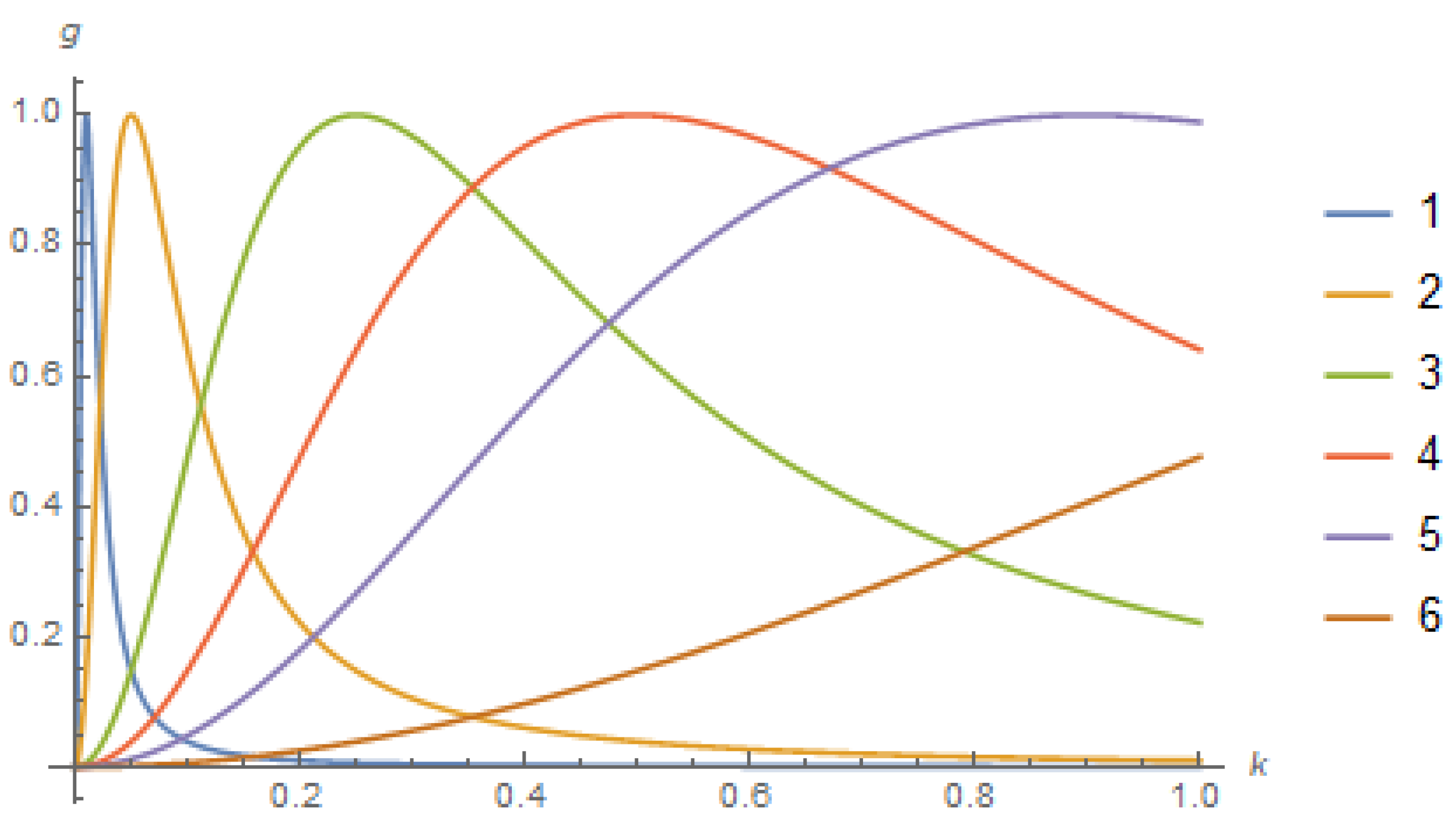
Since $sin{\left(\alpha \right)}^2\le 1$, $cos{\left(\beta \right)}^2\le 1$, the relation 2) imposes the restriction $f_{ext}\ge 2k_{max}$ on $f_{ext}$, and in case 1), the inequality $f_{est}\ge 2k_{max}/\sqrt{1-f_{max}}$ must be fulfilled. Thus, the function $\tilde{h}\left(k\right)$ can be presented in the form $\tilde{h}\left(k\right)=c_{1}g(c_2;k/c_3)$ with $0<c_1<1$, $0<c_2\le 1/4$, $0<c_3$. It is even: $\tilde{h}\left(k\right)=\tilde{h}(-k)$ has the maximum value ${\tilde{h}}_{max}=c_1$ by $\left|k\right|=c_3=k_{max}$, and the extension of the neighborhood of $k_{max}$ is $h_{ext}=c_3/\sqrt{c_2}$. By given $c_3$, the function $\tilde{h}\left(k\right)$ has the minimal value of $h_{ext}$ by $c_2=1/4$. If $c_2=1/4$, then $\tilde{h}\left(k\right)=h_{max}g(1/4,k/c_3)$.

The graphs of the functions $g(1/4,k/c)$ by different $c=k_{max}$ are shown on Figure 1. With an increase of c, the vicinity of the maxima becomes increasingly more flat, and the positions of the maxima become increasingly less noticeable. Using the notation

$$h(u_{1\pm },u_{2\pm },v_{1\pm },v_{2\pm };k)=h_{\pm }\left(k\right)=\tilde{h}(r_{\pm },{\alpha }_{\pm },{\beta }_{\pm };k)={\tilde{h}}_{\pm }\left(k\right)=c_{1\pm }g(c_{2\pm };k/c_{3\pm }),$$

one can present the functions $|t_{\mu \pm }{|}^2$ of $k_{\mu }$ in the form $|t_{\mu \pm }{|}^2=h_{\pm }\left(k_{\mu }\right)=g_{\pm }\left(k_{\mu }\right)=c_{1\pm }g(c_{2\pm };k_{\mu }/c_{3\pm })$ and obtain the following expression for the transmission coefficient:

$$\begin{array}{c}\hfill K_t\left(k\right)=c_{1+}g(c_{2+};k/c_{3+})cos{\left(\theta \right)}^2+c_{1-}g(c_{2-};k/c_{3-})sin{\left(\theta \right)}^2.\end{array}$$

Let us consider, as an example, a scattering process for which $\theta =0$ and $u_{1+}=0.5,u_{2+}=0.3,v_{1+}=0.01,v_{2+}=85$. In this case, ${\alpha }_{+}=0.00941038,{\beta }_{+}=-1.56844,r_{+}=4.442675$ and

$$\begin{array}{c}\hfill K_t\left(k\right)=h_{+}\left(k\right)=\frac{4}{4+0.2^2+{(\frac{0.01}{k}-85k)}^2}=\frac{c_{1+}}{1+c_{2+}{\left(\frac{c_{3+}}{k}-\frac{k}{c_{3+}}\right)}^2}=c_{1+}g(c_{2+};k/c_{3+}),\end{array}$$

(33)

$$\begin{array}{c}\hfill c_{1+}=\frac{4}{4.04}\approx 0.990099,c_{2+}=\frac{0.85}{4.04}\approx 0.210396,c_{3+}=\frac{1}{10\sqrt{85}}\approx 0.0108465.\end{array}$$

(34)

The maximal value of $K_t\left(k\right)$ is $h_{max+}=c_{1+}=h_{+}\left(k_m\right)$, $k_{max}=c_{3+}$, $h_{ext+}=\frac{c_{3+}}{\sqrt{c_{2+}}}=\frac{\sqrt{4.04}}{85}\approx 0.0236468$. The parameters $c_1,c_2,c_3$ (34) are very close to ones defining the function presented by Graphic 1 on the Figure 1. The difference between it and the graph of the function $K_t\left(k\right)$ (33) is inessential. Note that $c_{2+}$ (34) fulfill the restrictions $c_{2+}\le 1/4$ and $h_{ext}=\sqrt{4.04}/85\approx 0.0236>2k_{max}\approx 0.0216$. However, $2k_{max}/\sqrt{1-f_{mak}}\approx 0.218$ and the inequality $h_{ext}\sqrt{1-f_{mak}}\ge k_{max}$ is not satisfied. Therefore, there is only one $\{r,\alpha ,\beta \}$-parametrization ${\tilde{h}}_{+}(r,\alpha ,\beta ;k)$ of the function $h_{+}(u_1,u_2,v_1,v_2;k)$ in this case.

Outside the neighborhood, $0.00162<k<0.0726$ ( $0.00324<\rho <0.146$ ) of the point $k_{max}=0.0108$ (${\rho }_{max}=0.0217)$, $h_{+}\left(k\right)$ (33) is 10 times less than its maximum value. For $0.1<k<1$, it decreases monotonically from $h_{+}\left(0.1\right)=0.0536193$ to $h_{+}\left(1\right)=0.000553454$ and has the maximal value $h_{+\left(max\right)}$ at the point $0<c_{3+}<1$ (34).

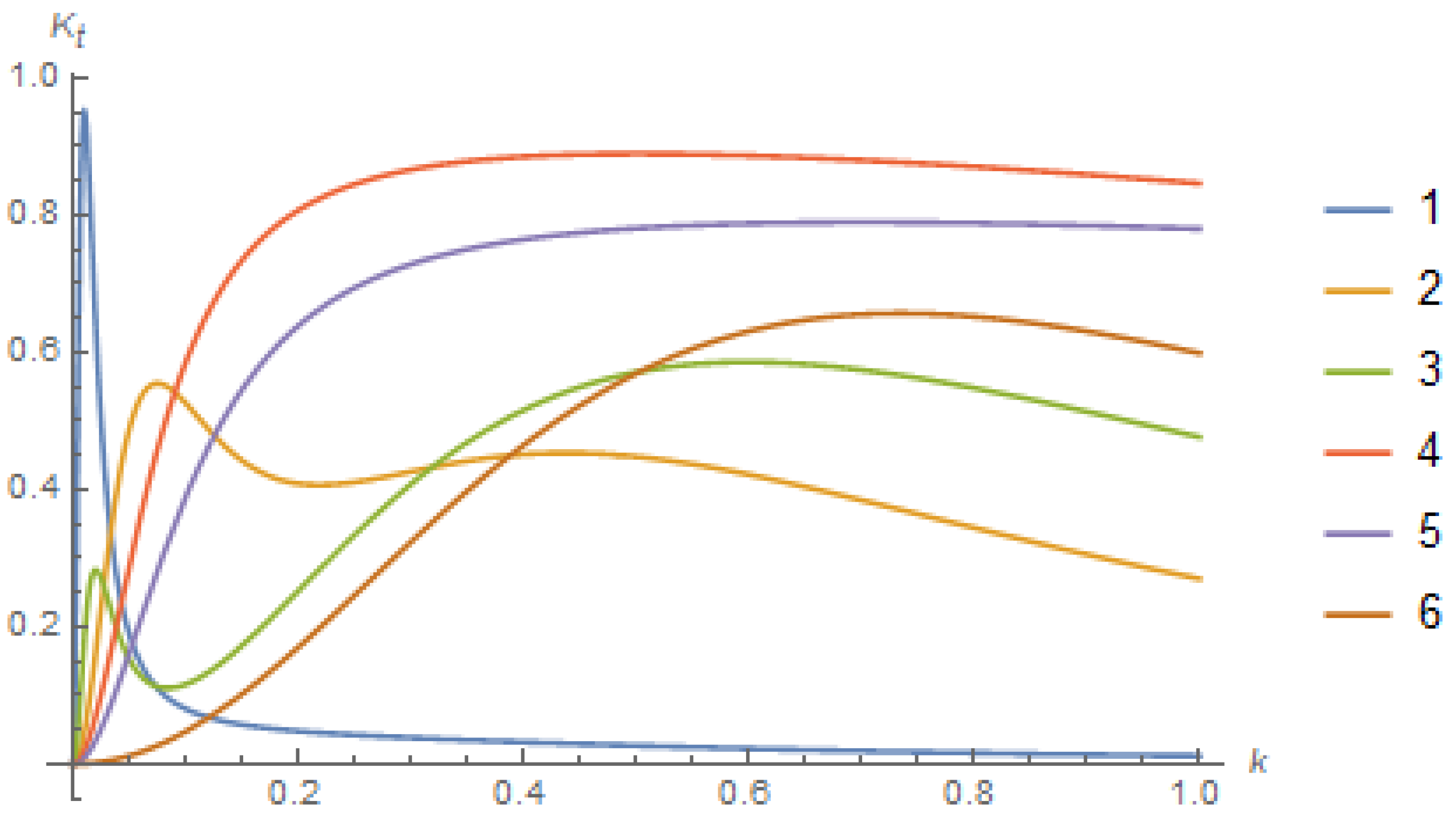
The graph of $h_{+}\left(k\right)$ (33) differs significantly from the (graphs (2)–(6)) shown in Figure 2 for $K_t\left(k\right)$ by $cos{\left(\theta \right)}^2\ne 1,0$. These ones can have two maxima (graphs (2) and (3)), one smoothed maximum (graph (6)), or change very little on the most part of the interval $0\le k\le 1$ (graphs (4) and (5)).

In the general case, the process of neutrino scattering on the plane is described by one universal function $g\left(k\right)=g(\alpha ,\beta ,k)$ parameterized by constants $0\le \alpha <0.25,\beta >0$: $K_t\left(k\right)=g({\alpha }_{-},{\beta }_{-},k){\gamma }_{-}+g({\alpha }_{+},{\beta }_{+},k){\gamma }_{+}$ with factors ${\gamma }_{\pm }>0$. In the terms of parameters $c_{1\pm },c_{2\pm },c_{3\pm },\theta$ used above, ${\alpha }_{\pm }=c_{{}_2\pm }$, ${\beta }_{\pm }=c_{{}_3\pm }$, ${\gamma }_{+}=c_{1+}cos{\left(\theta \right)}^2$, ${\gamma }_{-}=c_{1-}sin{\left(\theta \right)}^2$. The maximal value of $g\left(k\right)$ is $1=g(\alpha ,\beta ;\beta )$. The argument k of this function is $k=\sqrt{p_0-m}/\sqrt{p_0+m}$, where m is the mass of the particle and $p_0$ its energy. Hence, $0\le k<1$ by the physical values $m\le p_0<\infty$ of $p_0$. If $0<\beta \le 1$, then $g(\alpha ,\beta ;k)$ has the maximum on the interval $0<k\le 1$. If $\beta >1$, then $g(\alpha ,\beta ;k)$ grows from $g(\alpha ,\beta ;0)=0$ to $g(\alpha ,\beta ;\beta )=\alpha$ with an increase of k by $0<k\le 1$.

Since, in the considered scattering process m, $p^3$ and k fulfill the relations $k=\sqrt{p_0-m}/$$\sqrt{p_0+m}$, $p_0^2-p_3^2=m^2$, one can present $p^3$, $p^0$ as $p^0=(1+k^2)m/(1-k^2)$, $p^3=2km/(1-k^2)$. Hence, if $g(\alpha ,\beta ;k)=1$, then $k=\beta$ and $p^0=(1+{\beta }^2)m/(1-{\beta }^2)$, $p^3=2\beta m/(1-{\beta }^2)$.

Corresponding to (33) function $K_t\left(p\right)$, the transmission coefficient as functions of $p^3$ has the maximum by $p^3=2c_{3+}m/(1-c_{3+}^2)=20\sqrt{85}m/8499\approx 0.0216956$ m, and as the function of $p^0$, it is maximal by $p^0=(1+c_{3+}^2)m/(1-c_{3+}^2)=8501m/8499\approx 1.00024m$.

Now, we analyze the features of system dynamics in the framework of the flavor representation. As the matrices $\Gamma$ used in (2) when discussing the oscillation process of neutrinos, we consider $\Gamma =I,{\gamma }^0,{\gamma }^3;{\gamma }^5,{\gamma }^0{\gamma }^5,{\gamma }^3{\gamma }^5$. The function ${\overline{\chi }}_{\mu }\left(p_{\mu }\right){\chi }_{\mu }\left(p_{\mu }\right)$$\left({\overline{\chi }}_{\mu }\left(p_{\mu }\right){\gamma }^5{\chi }_{\mu }\left(p_{\mu }\right)\right)$ is interpreted as the scalar (pseudo-scalar) density of the $\mu$-$\mathit{th}$ particles with momentum $p_{\mu }=\{p_{\mu }^0,0,0,p^3\}$, ${\overline{\chi }}_{\mu }\left(p_{\mu }\right)\{{\gamma }^0,0,0,{\gamma }^3\}{\chi }_{\mu }\left(p_{\mu }\right)$ (${\overline{\chi }}_{\mu }\left(p_{\mu }\right)\{{\gamma }^0{\gamma }^5,0,0,{\gamma }^3{\gamma }^5\}{\chi }_{\mu }\left(p_{\mu }\right)$) is the four-current vector (axial four-current pseudo-vector) of the $\mu$-$\mathit{th}$ particles moving along the $x^3$-axis. We will use the plane wave presentation for spinors ${\overline{\chi }}_{\mu }\left(p_{\mu }\right),{\chi }_{{\mu }^{\prime }}\left(p_{{\mu }^{\prime }}\right)$ describing the particles with momentum $p^3$ moving orthogonal to the plane $x^3=0$:

$$\begin{array}{c}\hfill {\chi }_{\mu }=e^{i{\rho }_{\mu }}({\sigma }_{1\mu }{\alpha }_{1\mu }+{\sigma }_{2\mu }{\alpha }_{2\mu }),{\overline{\chi }}_{\mu }=e^{-i{\rho }_{\mu }}({\sigma }_{1\mu }{\alpha }_{1\mu }^{*}+{\sigma }_{2\mu }{\alpha }_{2\mu }^{*}){\gamma }^0,\\ \hfill {\sigma }_{1\mu }=\left\{\begin{array}{c}1\\ 0\\ k_{\mu }\\ 0\end{array}\right\},{\sigma }_{2\mu }=\left\{\begin{array}{c}0\\ 1\\ 0\\ -k_{\mu }\end{array}\right\},k_{\mu }=\frac{p^3}{p_{\mu }^0+m_{\mu }},p_{\mu }^0=\sqrt{{\left(p^3\right)}^2+m_{\mu }^2},\\ \hfill k_{\mu }=\frac{1}{2}\frac{p^3}{m_{\mu }}-\frac{1}{8}{\left(\frac{p^3}{m_{\mu }}\right)}^3+\mathcal{O}{\left(\frac{p^3}{m_{\mu }}\right)}^4,k_{\mu }=1-\frac{m_{\mu }}{p^3}+\frac{1}{2}{\left(\frac{m_{\mu }}{p^3}\right)}^2+\mathcal{O}{\left(\frac{m_{\mu }}{p^3}\right)}^4.\end{array}$$

By means of notation ${\mathbf{a}}_{\mu {\mu }^{\prime }}^{\pm }={\alpha }_{1\mu }^{*}{\alpha }_{1{\mu }^{\prime }}\pm {\alpha }_{2\mu }^{*}{\alpha }_{2{\mu }^{\prime }}$, the results obtained for the ${\overline{\chi }}_{\mu }\left(p_{\mu }\right)\Gamma {\chi }_{{\mu }^{\prime }}\left(p_{{\mu }^{\prime }}\right)$ are written in the form

$$\begin{array}{c}\hfill {\overline{\chi }}_{\mu }{\chi }_{{\mu }^{\prime }}=\left(1-k_{\mu }{k}_{{\mu }^{\prime }}\right)e^{i({\rho }_{{\mu }^{\prime }}-{\rho }_{\mu })}{\mathbf{a}}_{\mu {\mu }^{\prime }}^{+},\\ \hfill {\overline{\chi }}_{\mu }{\gamma }^0{\chi }_{{\mu }^{\prime }}=\left(1+k_{\mu }{k}_{{\mu }^{\prime }}\right)e^{i({\rho }_{{\mu }^{\prime }}-{\rho }_{\mu })}{\mathbf{a}}_{\mu {\mu }^{\prime }}^{+},{\overline{\chi }}_{\mu }{\gamma }^3{\chi }_{{\mu }^{\prime }}=\left(k_{\mu }+k_{{\mu }^{\prime }}\right)e^{i({\rho }_{{\mu }^{\prime }}-{\rho }_{\mu })}{\mathbf{a}}_{\mu {\mu }^{\prime }}^{+}\end{array}$$

and

$$\begin{array}{c}\hfill {\overline{\chi }}_{\mu }{\gamma }_5{\chi }_{{\mu }^{\prime }}=\left(k_{\mu }-k_{{\mu }^{\prime }}\right)e^{i({\rho }_{{\mu }^{\prime }}-{\rho }_{\mu })}{\mathbf{a}}_{\mu {\mu }^{\prime }}^{-},\\ \hfill {\overline{\chi }}_{\mu }{\gamma }^0{\gamma }_5{\chi }_{{\mu }^{\prime }}=\left(k_{\mu }+k_{{\mu }^{\prime }}\right)e^{i({\rho }_{{\mu }^{\prime }}-{\rho }_{\mu })}{\mathbf{a}}_{\mu {\mu }^{\prime }}^{-},{\overline{\chi }}_{\mu }{\gamma }^3{\gamma }_5{\chi }_{{\mu }^{\prime }}=\left(1+k_{\mu }{k}_{{\mu }^{\prime }}\right)e^{i({\rho }_{{\mu }^{\prime }}-{\rho }_{\mu })}{\mathbf{a}}_{\mu {\mu }^{\prime }}^{-}.\end{array}$$

Oscillations of incident waves are presented by ${\overline{\psi }}_{\lambda }\left(x\right)\Gamma {\psi }_{\lambda }\left(x\right)={\sum }_{\mu ,{\mu }^{\prime }}^3{e}_{\mu \lambda }^{*}{e}_{{\mu }^{\prime }\lambda }{\overline{\varphi }}_{\mu }\left(x\right)\Gamma {\varphi }_{{\mu }^{\prime }}\left(x\right)$ as

$$\begin{array}{c}\hfill {\overline{\psi }}_{\lambda }\left(x\right){\psi }_{\lambda }\left(x\right)=\sum _{\mu =1}^3{e}_{\mu \lambda }^{*}{e}_{\mu \lambda }\left(1-k_{\mu }^2\right){\mathbf{a}}_{\mu \mu }^{+}+\sum _{\mu \ne {\mu }^{\prime }=1}^3{e}^{i(p_{\mu }^0-p_{{\mu }^{\prime }}^0)x^0}{e}_{\mu \lambda }^{*}{e}_{{\mu }^{\prime }\lambda }\left(1-k_{\mu }{k}_{{\mu }^{\prime }}\right)e^{i({\rho }_{{\mu }^{\prime }}-{\rho }_{\mu })}{\mathbf{a}}_{\mu {\mu }^{\prime }}^{+},\\ \hfill {\overline{\psi }}_{\lambda }\left(x\right){\gamma }^0{\psi }_{\lambda }\left(x\right)=\sum _{\mu =1}^3{e}_{\mu \lambda }^{*}{e}_{\mu \lambda }\left(1+k_{\mu }^2\right){\mathbf{a}}_{\mu \mu }^{+}+\sum _{\mu \ne {\mu }^{\prime }=1}^3{e}^{i(p_{\mu }^0-p_{{\mu }^{\prime }}^0)x^0}{e}_{\mu \lambda }^{*}{e}_{{\mu }^{\prime }\lambda }\left(1+k_{\mu }{k}_{{\mu }^{\prime }}\right)e^{i({\rho }_{{\mu }^{\prime }}-{\rho }_{\mu })}{\mathbf{a}}_{\mu {\mu }^{\prime }}^{+},\\ \hfill {\overline{\psi }}_{\lambda }\left(x\right){\gamma }^3{\psi }_{\lambda }\left(x\right)=2\sum _{\mu =1}^3{e}_{\mu \lambda }^{*}{e}_{\mu \lambda }{k}_{\mu }{\mathbf{a}}_{\mu \mu }^{+}+\sum _{\mu \ne {\mu }^{\prime }=1}^3{e}^{i(p_{\mu }^0-p_{{\mu }^{\prime }}^0)x^0}{e}_{\mu \lambda }^{*}{e}_{{\mu }^{\prime }\lambda }\left(k_{\mu }+k_{{\mu }^{\prime }}\right)e^{i({\rho }_{{\mu }^{\prime }}-{\rho }_{\mu })}{\mathbf{a}}_{\mu {\mu }^{\prime }}^{+}.\end{array}$$

(35)

and

$$\begin{array}{c}\hfill {\overline{\psi }}_{\lambda }\left(x\right){\gamma }_5{\psi }_{\lambda }\left(x\right)=\sum _{\mu \ne {\mu }^{\prime }=1}^3{e}^{i(p_{\mu }^0-p_{{\mu }^{\prime }}^0)x^0}{e}_{\mu \lambda }^{*}{e}_{{\mu }^{\prime }\lambda }\left(k_{\mu }-k_{{\mu }^{\prime }}\right)e^{i({\rho }_{{\mu }^{\prime }}-{\rho }_{\mu })}{\mathbf{a}}_{\mu {\mu }^{\prime }}^{-},\\ \hfill {\overline{\psi }}_{\lambda }\left(x\right){\gamma }^0{\gamma }_5{\psi }_{\lambda }\left(x\right)=2\sum _{\mu =1}^3{e}_{\mu \lambda }^{*}{e}_{\mu \lambda }{k}_{\mu }{\mathbf{a}}_{\mu \mu }^{-}+\sum _{\mu \ne {\mu }^{\prime }=1}^3{e}^{i(p_{\mu }^0-p_{{\mu }^{\prime }}^0)x^0}{e}_{\mu \lambda }^{*}{e}_{{\mu }^{\prime }\lambda }\left(k_{\mu }+k_{{\mu }^{\prime }}\right)e^{i({\rho }_{{\mu }^{\prime }}-{\rho }_{\mu })}{\mathbf{a}}_{\mu {\mu }^{\prime }}^{-},\\ \hfill {\overline{\psi }}_{\lambda }\left(x\right){\gamma }^3{\gamma }^5{\psi }_{\lambda }\left(x\right)=\sum _{\mu =1}^3{e}_{\mu \lambda }^{*}{e}_{\mu \lambda }\left(1+k_{\mu }^2\right){\mathbf{a}}_{\mu \mu }^{-}+\sum _{\mu \ne {\mu }^{\prime }=1}^3{e}^{i(p_{\mu }^0-p_{{\mu }^{\prime }}^0)x^0}{e}_{\mu \lambda }^{*}{e}_{{\mu }^{\prime }\lambda }\left(1+k_{\mu }{k}_{{\mu }^{\prime }}\right)e^{i({\rho }_{{\mu }^{\prime }}-{\rho }_{\mu })}{\mathbf{a}}_{\mu {\mu }^{\prime }}^{-}.\end{array}$$

(36)

For transmitted waves, one needs to replace $a_{1\mu }\to c_{1\mu }=t_{\mu +}{a}_{1\mu },a_{2\mu }\to c_{2\mu }=t_{\mu -}{a}_{2\mu }$. Thus, changing in (35) and (36)

$$\begin{array}{c}\hfill {\mathbf{a}}_{\mu {\mu }^{\prime }}^{\pm }\to {\mathbf{c}}_{\mu {\mu }^{\prime }}^{\pm }=c_{1{\mu }^{\prime }}^{*}{c}_{1\mu }\pm c_{2{\mu }^{\prime }}^{*}{c}_{2\mu }=\left(t_{{\mu }^{\prime }+}^{*}{t}_{\mu +}\right)a_{1{\mu }^{\prime }}^{*}{a}_{1\mu }\pm \left(t_{{\mu }^{\prime }-}^{*}{t}_{\mu -}\right)a_{2{\mu }^{\prime }}^{*}{a}_{2\mu },\end{array}$$

one receives the corresponding results for transmitted neutrino oscillations. If $m_1<m_2<m_3$ and momentum $p^3$ is the same for all particles, then $p^3/m_1>p^3/m_2>p^3/m_3$. For given $p^3$, we denote $k_{\mu }=p^3/(m_{\mu }+\sqrt{{\left(p^3\right)}^2+m_{\mu }^2})$, $\mu =1,2,3$. If $|t_{\pm }{|}^2\left(k\right)$ monotonically increases from zero to $|t_{\pm }{|}^2\left(1\right)$ by $0\le k\le 1$, then $|t_{\pm }{|}^2\left(k_1\right)>|t_{\pm }{|}^2\left(k_2\right)>{\left|t_{\pm }\right|}^2\left(k_3\right)$, since $k_1>k_2>k_3$. In virtue of

$$\begin{array}{c}\hfill |t_{\pm }{|}^2\left(k_1\right)-|t_{\pm }{|}^2\left(k_2\right)=(k_1-k_2)\frac{\partial }{\partial k}{\left|t_{\pm }\right|}^2\left(k\right){|}_{k=k^{\prime }},k_1>k^{\prime }>k_2,\\ \hfill |t_{\pm }{|}^2\left(k_2\right)-|t_{\pm }{|}^2\left(k_3\right)=(k_2-k_3)\frac{\partial }{\partial k}{\left|t_{\pm }\right|}^2\left(k\right){|}_{k=k^{″}},k_2>k^{″}>k_3,\end{array}$$

the greater the derivatives of the function $|t_{\pm }{|}^2\left(k\right)$ are at points $k^{\prime }$ and $k^{\prime \prime }$ for given $k_1,k_2,k_3,$ that is, the faster $|t_{\pm }{|}^2\left(k\right)$ grows on the interval $k_1>k>k_3$, the more there will be an influence of the neutrino collisions with the plane on the process of their oscillations.

If there is a maximum of $|t_{\pm }{|}^2\left(k\right)$ by $0<k<1$, then each $|t_{\pm }{|}^2\left(k_{\mu }\right)$, $\mu =1,2,3$ can be maximal, and the following situations are possible:

(1)

$|t_{\pm }{|}^2\left(k_1\right)$ is maximal, $|t_{\pm }{|}^2\left(k_3\right)<|t_{\pm }{|}^2\left(k_2\right)<{\left|t_{\pm }\right|}^2\left(k_1\right)$;

(2)

$|t_{\pm }{|}^2\left(k_2\right)$ is maximal, $|t_{\pm }{|}^2\left(k_3\right)<|t_{\pm }{|}^2\left(k_1\right)<{\left|t_{\pm }\right|}^2\left(k_2\right)$

or $|t_{\pm }{|}^2\left(k_1\right)<|t_{\pm }{|}^2\left(k_3\right)<{\left|t_{\pm }\right|}^2\left(k_2\right)$;

(3)

$|t_{\pm }{|}^2\left(k_3\right)$ is maximal, $|t_{\pm }{|}^2\left(k_1\right)<|t_{\pm }{|}^2\left(k_2\right)<{\left|t_{\pm }\right|}^2\left(k_3\right)$.

The more the function $|t_{\pm }{|}^2\left(k\right)$ resembles an approximation of the delta-function and the nearer the maximal $|t_{\pm }{|}^2\left(k_{\mu }\right)$ is to the maximum of $|t_{\pm }{|}^2\left(k\right)$, the greater is the difference of maximal $|t_{\pm }{|}^2\left(k_{\mu }\right)$ from non-maximal $|t_{\pm }{|}^2\left(k_{{\mu }^{\prime }}\right)$, and the more significant will be the changes in neutrino oscillations as a result of their collisions with the plane.

We considered the model with 8 real parameters in the matrix Q (6). It could be interesting to compare its properties with features of the system with matrices Q of the form (7)–(9). In the case (7), there are four real parameters defining Q and

$$\begin{array}{c}\hfill S_{\pm }^{(\pm )}=e^{i\eta }({\varsigma }_0{\tau }_0^{(\pm )}+i{\varsigma }_1{\tau }_1^{(\pm )}\pm {\varsigma }_2{\tau }_2^{(\pm )}\pm {\varsigma }_3{\tau }_3^{(\pm )}),\end{array}$$

(37)

$$\begin{array}{c}\hfill u_{1+}=u_{2-}={\varsigma }_0+{\varsigma }_3=u_1,u_{2+}=u_{1-}={\varsigma }_0-{\varsigma }_3=u_2,\end{array}$$

(38)

$$\begin{array}{c}\hfill v_{1+}=v_{2-}={\varsigma }_1+{\varsigma }_2=v_1,v_{2+}=v_{1-}={\varsigma }_1-{\varsigma }_2=v_2,\end{array}$$

(39)

$$\begin{array}{c}\hfill {\varsigma }_0=cosh\left(r\right)cos\left(\alpha \right),{\varsigma }_1=cosh\left(r\right)sin\left(\alpha \right),{\varsigma }_2=sinh\left(r\right)cos\left(\beta \right),{\varsigma }_3=sinh\left(r\right)sin\left(\beta \right).\end{array}$$

(40)

Here, ${\varsigma }_0,{\varsigma }_1,{\varsigma }_2,{\varsigma }_3$, $u_1,u_2,v_1,v_2$ are real parameters fulfilled the conditions ${\varsigma }_0^2+{\varsigma }_1^2-{\varsigma }_2^2-{\varsigma }_3^2=1$, $u_1{u}_2+v_1{v}_2=1$ and $r\ge 0,0\le \alpha \le 2\pi ,0\le \beta \le 2\pi$, $0\le \eta \le \pi$. Hence, for such materials,

$$\begin{array}{c}\hfill t_{\mu +}=t_{\mu -}^{*}=\frac{2i{k}_{\mu }}{k_{\mu }^2{v}_2+i{k}_{\mu }(u_1+u_2)+v_1}=t_{\mu },{\left|t_{\mu }\right|}^2=\frac{4}{4+{(u_1-u_2)}^2+{(\frac{v_1}{k_{\mu }}-k_{\mu }{v}_2)}^2}=K_{t_{\mu }},\\ \hfill |r_{\mu +}{|}^2=|r_{\mu -}{|}^2={\left|r_{\mu }\right|}^2=K_{r_{\mu }}=1-K_{t_{\mu }},{\mathbf{c}}_{\mu {\mu }^{\prime }}^{\pm }=\left(t_{{\mu }^{\prime }}^{*}{t}_{\mu }\right)a_{1{\mu }^{\prime }}^{*}{a}_{1\mu }\pm \left(t_{{\mu }^{\prime }}{t}_{\mu }^{*}\right)a_{2{\mu }^{\prime }}^{*}{a}_{2\mu }.\end{array}$$

Putting $\eta =0,{\varsigma }_1=0,\alpha =0$ in (37)–(40), one obtains for the model given by matrix Q (8) with two real parameters

$$\begin{array}{c}\hfill S_{\pm }^{(\pm )}={\varsigma }_0{\tau }_0^{(\pm )}\pm {\varsigma }_2{\tau }_2^{(\pm )}\pm {\varsigma }_3{\tau }_3^{(\pm )},{\varsigma }_0=cosh\left(r\right),{\varsigma }_2=sinh\left(r\right)cos\left(\beta \right),{\varsigma }_3=sinh\left(r\right)sin\left(\beta \right)\end{array}$$

(41)

$$\begin{array}{c}\hfill u_1={\varsigma }_0+{\varsigma }_3,u_2={\varsigma }_0-{\varsigma }_3,v_1={\varsigma }_2=v,v_2=-{\varsigma }_2=-v,\end{array}$$

(42)

with real ${\varsigma }_0,{\varsigma }_2,{\varsigma }_3$, $u_1,u_2,v$ fulfilling the conditions ${\varsigma }_0^2-{\varsigma }_2^2-{\varsigma }_3^2=1$, $u_1{u}_2-v^2=1$, and $r\ge 0$, $0\le \beta \le 2\pi$. In this model,

$$\begin{array}{c}\hfill t_{\mu +}=t_{\mu -}^{*}=\frac{2i{k}_{\mu }}{i{k}_{\mu }(u_1+u_2)+v(1-k_{\mu }^2)}=t_{\mu },{\left|t_{\mu }\right|}^2=\frac{4}{4+{(u_1-u_2)}^2+v^2{(\frac{1}{k_{\mu }}+k_{\mu })}^2}=K_{t_{\mu }}.\end{array}$$

If one sets in (41) and (42) ${\varsigma }_3=0,\beta =0$, then one receives, for the model with a matrix Q (9) containing one real parameter,

$$\begin{array}{c}\hfill S_{\pm }^{(\pm )}={\varsigma }_0{\tau }_0^{(\pm )}\pm {\varsigma }_2{\tau }_2^{(\pm )},{\varsigma }_0=cosh\left(r\right),{\varsigma }_2=sinh\left(r\right),u_1=u_2={\varsigma }_0=u,v_1=-v_2={\varsigma }_2=v.\end{array}$$

Here, ${\varsigma }_0,{\varsigma }_2$, $u,v$ are real parameters, ${\varsigma }_0^2-{\varsigma }_2^2=1$, $u^2-v^2=1$ and $r\ge 0$. In this case,

$$\begin{array}{c}\hfill t_{\mu }=\frac{2i{k}_{\mu }}{2iu{k}_{\mu }+v(1-k_{\mu }^2)},{\left|t_{\mu }\right|}^2=\frac{4}{4+v^2{(\frac{1}{k_{\mu }}+k_{\mu })}^2}=K_{t_{\mu }}.\end{array}$$

The essential difference between the models with matrix Q of the form (6)–(9) is that the functions $|t_{\mu \pm }{|}^2\left(k\right),{\left|t_{\mu }\right|}^2\left(k\right)$, in the models (6), (7) can have the maximum by $0<k<1$, but $|t_{\mu }{|}^2\left(k\right)$ in models (8), (9) are, by $0\le k\le 1$, the monotonously growing functions.

8. Conclusions

In our work, we considered the problem of neutrino interaction with matter. Using our experience in constructing models of QED in singular background fields, we have proposed a quantum-field approach, which may be useful for the theoretical description of neutrino propagation in a highly inhomogeneous medium. It assumes taking into account the basic symmetry principles of modern physics of fundamental interactions that underlie the Standard Model and can, in principle, be generalized to describe the interaction of all lepton fields with the external environment. Mainly, attention was paid to the problem of neutrino scattering on a material plane, considered as a simplest example of process in the space with a strongly inhomogeneous distribution of substance.

In a general form, for a model with an off-diagonal unitary matrix $\Lambda$ mixing Dirac fields in the mass representation, expressions for the reflected and transmitted waves were obtained. For them, in the model with a diagonal $\Lambda$, an explicit solution was obtained, which was used to analyze the oscillations of neutrinos in the case of their motion, orthogonally to the plane $x^3=0$. It was shown that the parameters that determine the material properties of the plane can be chosen so that its effect on the neutrino flux is similar to a filter that transmits particles in a narrow interval of low energies and almost completely reflects all other ones. As a result of the neutrino collision with the plane, the parallel component of the momentum does not change, and the orthogonal one does not change in absolute value. Only the amplitudes of fields can change significantly.

The example we have considered with parameters of the model (33) and (34) shows that the interaction of neutrinos with a plane can effect their filtration. A characteristic feature of the filtration process of particles upon collision with a plane is the possibility of essentially different transmission coefficients for neutrinos of different masses. In this case, due to filtration of their flux, the regimes of the neutrino oscillations before the plane and behind it can be strongly different. This phenomenon can be used to estimate the masses of neutrinos of various types in carrying out analyses of experimental data.

Although the filtering and MSW-resonance results are similar in many ways, their mechanics are not the same. The MSW effect is formed non-locally in space and time. This requires a certain volume of matter and a certain period of time, generally speaking, that are different for various substances. In order for the filtration of the neutrino flux to occur, their collision with the plane is sufficient, which (in the framework of the considered model) occurs instantaneously and locally at $x^3=0$. From the point of view of the possibility of verifying the adequacy of the proposed model, it would be interesting to reveal in the dynamics of neutrino oscillations an effect, which cannot arise as a consequence of MSW resonance and is a manifestation of the filtration process.

One of the current theoretical problems in neutrino astro-physics is constructing numerical models of dynamics of supernova explosions. Many research teams have been working on this issue [52,53,54,55,56,57,58,59,60,61,62,63,64,65,66,67]. Perhaps, taking into account the filtering mechanism in such models will be useful to achieve a better understanding of the features of the process of collapse of the super-heavy star core.

In general terms, a possible scenario of its evolution can be presented as follows. If, in the core of the star, its shell filters neutrinos by energies, they can be divided into two classes. Particles with energies from the narrow range of the low-energy region leave the core unhindered. These neutrinos can be called free. For all the others, which we will call bound, the core shell is impermeable.

In the process of the star’s evolution, its core is subjected to the pressure of the increasing gravitational forces. In it, neutrinos are born, the free ones are emitted, and the bound neutrinos are accumulated in the core. This can go on until the main features of the interaction between the core shell and neutrinos changes, the class of free neutrinos expands, and the star will emit them with further contraction without a significant change in its structure. In our model, this can be described by changing the function $K_t\left(k\right)$. For instance, if the plots of possible $K_t\left(k\right)$, is shown in Figure 2, then within the change $\left(1\right)\to \left(4\right)$, a large fraction of the bound high-energy neutrinos become free, they will leave the star, essentially changing the intensity and spectrum of its neutrino emission.

If the main interaction features of neutrinos with the core shell are not changed and at least some of the bound neutrinos do not become free, then the enormous energy accumulated by them in the core destroys its shell sooner or later. After that, the core and the star are exploded.

There is great interest among experimentalists to determine neutrino masses directly [68,69,70,71,72]. One can assume that the employment of 2D materials and special surface treatment techniques in the construction of neutrino detectors would enable one to efficiently use the filtering mechanism in experiments of such a kind.

The maximal number of parameters in the model, the properties of which we have studied in detail, was eight for the matrix Q and three for the diagonal matrix $\Lambda$. Not all of them are included in our results, and the question arises whether it is possible to reduce the number of parameters in the model without limiting its area of applicability. We considered versions of the model with four, two, and one parameters in the Q matrix, simplified for symmetry reasons, and found a difference in the properties of their predicted transmission coefficients. This raises the question of whether one can confine oneself to using the simplest models to describe real neutrino oscillation data.

We suppose that the proposed method for modeling the processes of interaction of neutrinos with matter can be useful for theoretical studies and analysis of the obtained experimental data.