Abstract
Intense electric fields applied to an asymmetric π-cell containing a nematic liquid crystal subjected to strong mechanical stresses induce distortions that are relaxed through a fast-switching mechanism: the order reconstruction transition. Topologically different nematic textures are connected by such a mechanism that is spatially driven by the intensity of the applied electric fields and by the anchoring angles of the nematic molecules on the confining plates of the cell. Using the finite element method, we implemented the moving mesh partial differential equation numerical technique, and we simulated the nematic evolution inside the cell in the context of the Landau–de Gennes order tensor theory. The order dynamics have been well captured, putting in evidence the possible existence of a metastable biaxial state, and a phase diagram of the nematic texture has been built, therefore confirming the appropriateness of the used technique for the study of this type of problem.
1. Introduction
Bistable behaviors in nematic liquid crystals (NLCs) play a crucial role for their optical and switching properties. They can arise in the biaxial domains of such materials as a consequence of distortions of the nematic texture when the biaxial coherence length ξb is comparable to the length scale of the nematic distortion [1]. In fact, thermotropic NLCs are rod-like molecules possessing cylindrical symmetry and exhibiting orientational order. For such reason, a dimensionless unit vector n, the director, is identified as suitable to describe the NLC long axis average orientation in most electro-optical phenomena, while the scalar order parameter S accounts for the degree of order along the n direction. Due to the cylindrical symmetry, NLCs are said to be uniaxial [2], as they possess a unique optical axis.
On the other hand, local and continuous changes of the director orientation inside uniaxial nematic textures can happen [3,4,5,6,7,8,9,10]. By applying a distortion capable to break the uniaxial symmetry, two distinct optical axes arise inside the NLCs, giving rise to bistable behaviors which lower the degree of order, and their description is made by coupling the n and S parameters in the frame of the Landau–de Gennes order tensor theory [2,11].
The optical and switching properties of NLCs are experimentally investigated using the π-cell, a device in which a thin nematic film is confined between two flat glass plates. In order to obtain on both surfaces a nematic alignment exhibiting strong anchoring energy and a given pre-tilt angle θ, the internal surfaces are appropriately treated [12]. The generation of a splayed texture is ensured by an anti-parallel arrangement of the two plates [12] (Figure 1a). Such a configuration permits the existence of a second texture which is topologically distinct from the first one, where the nematic is π-twisted (or π-bent) (Figure 1c), while any spontaneous relaxation from each other is prevented by the energy barrier existing between them. The splayed texture can be transformed into the topologically different bent texture under the action of an electric field applied perpendicular to the boundary plates, a textural switch mediated by the biaxial order reconstruction (Figure 1b), a mechanism which connects two competing uniaxial textures through a wealth of transient biaxial states in the nanometric scale [12], and allowing for changing the local order of the nematic phase, avoiding any macroscopic rotation of the unit vector n. More generally, studies putting forth evidence of biaxial structural transitions induced by electric [13,14,15,16] or mechanical fields [17], growth of biaxial domains in the bulk and at the NLC interface [18,19,20,21], or surface effects [22,23] have been performed, while it is also found that further relaxation mechanisms become possible if strong anchoring asymmetries operate [22,23,24].
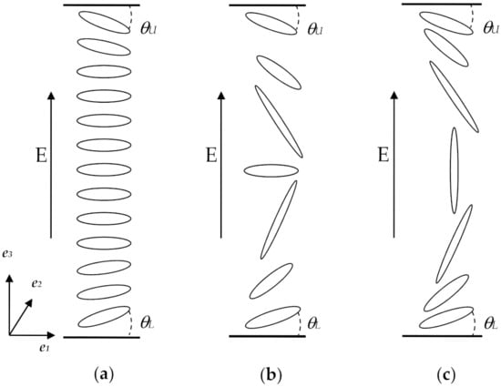
Figure 1.
Geometry of the π-cell with nematic molecules in different states: (a) horizontal alignment with a slight splay; (b) intermediate state with a thin wall in the center; and (c) mostly vertical alignment (π-bent).
In a recent series of papers [24,25,26,27], we studied the order dynamics of a 5CB NLC confined inside a π-cell and solved the partial differential equation (PDE) system arising from the modeling, implementing the moving mesh PDE (MMPDE) numerical technique using the finite element method (FEM). Such an adaptive grid technique, which is of the r-type [28], relies on domain discretization typical of the FEM in which the number of mesh points is kept constant; the nodes instead move driven by a monitor function, a suitable functional of the order parameter (in our case of the order gradient ∇Q) which causes the nodes to cluster toward regions with growing ∇Q, where greater accuracy is required, and vice versa. This results in an efficient and effective numerical tool, which is appropriate to model the order dynamics of the liquid crystals confined between plates, allowing reliable results to be obtained, aside from resolution improvement [25]. Moreover, with respect to computational techniques based on uniform discretizations, the MMPDE method allows computational savings. In fact, the domain regions of growing ∇Q are a priori unknown, but the mesh points are moved from time to time toward regions of high variability, always keeping them constant in number. The order dynamics of a nematic confined in a π-cell with symmetric [26,27] or asymmetric [24] anchoring angles has been studied using the MMPDE technique. Denoting with Eth a threshold level for applied electric field (AEF) amplitudes above which an order reconstruction transition occurs in the bulk of an NLC confined in a π-cell with symmetric anchoring conditions [12], applied fields with amplitudes not too far beyond Eth induce distortions in the cell center, which relax by means of an order reconstruction transition [26]. AEFs with higher amplitudes are instead capable of inducing other phenomena, such as delocalization of the order reconstruction transition, transient order lowering, and transitions of the nematic textures from splay to bend configuration (Figure 1), exhibiting first- and second-order features [27]. On the other hand, if asymmetric pre-tilt angles are imposed on the π-cell, the nematic distortion relaxes by means of a growing biaxiality propagating toward the boundary surface, identified by the smaller anchoring angle [23]. At this stage, depending on the choice of the amplitude of the applied electric pulse E and of the pre-tilt angle θU, the planar nematic texture imposed on the boundary surface can be connected to the nematic molecules aligned vertically along the field direction through either a bulk- or surface-order reconstruction transition [24]. Further, monitoring the order evolution as a function of the applied electric pulse amplitude E and the anchoring angle of the nematic on the upper boundary surface θU allows one to clearly distinguish bulk- from surface-order reconstruction occurring in the cell and to compute a partial phase diagram in which the nematic texture is mapped according to its switching mechanism [24]. In particular, we obtained a partition of the (E,θU) plane in regions where the modeled nematic texture obeys mechanisms with bulk switching, surface switching, or no switching at all. Nevertheless, the mapped region is a limited part of the phase diagram whose extension requires the investigation of more and more (E,θU) pairs in order to predict the phase boundaries among all possible switching regimes. Since increasing amplitudes of the applied electric pulse, as well as the marked asymmetries, induce nano-confined strong distortions in the NLC [23,24,27], being the scale of the physical problem, instead, in the micrometer range, a sophisticated computational technique is needed to obtain more reliable results. Following such an idea, in this work, we simulated a 5CB NLC confined in an asymmetric π-cell and subjected it to AEFs with amplitudes extending far beyond Eth. The time-dependent governing equations have been solved using the MMPDE numerical technique, and the biaxial order dynamics as well as the Q-eigenvalues have been monitored while imposing variable degrees of asymmetry. Moreover, being the order reconstruction transition confined within the duration of the applied electric pulse, material flow effects have been neglected [29].
2. The Mathematical Model
Globally, the order and orientation of biaxial nematics are described by the second-rank tensor Q, which is symmetric and traceless, according to the Landau–de Gennes theory [2,30]:
Each ei of the orthonormal basis of the Q eigenvectors {e1, e2, e3} lies along the directions of the preferred molecular orientation, assumed to be pointing along the x, y, and z directions of the laboratory frame of reference, respectively, while the degree of order along such directions is represented by the eigenvalues si. Nematics can be found in three different phases—isotropic, uniaxial, or biaxial—each associated to the si values. When they are in the isotropic phase, then each si = 0, and the optical behavior is an ordinary isotropic fluid. Uniaxial nematics have a unique optical axis, identified by the eigenvector ei = n, associated to the maximum eigenvalue smax, giving in turn the scalar order parameter S = (3/2) smax. Finally, biaxial nematics all have different eigenvalues.
Modeling the dynamical evolution of the Q-tensor encompasses the NLC free energy density F minimization [2]. Imposing fixed boundary conditions to the cell surfaces results in infinite anchoring energy for the NLC molecules. For this reason, we assume that contributions to F arise only from the bulk, thus neglecting surface terms, and the ion effects are neglected, considering the nematic as a purely dielectric material [12]. Hence, the following is true:
where
are thermotropic, elastic, and electric contributions, respectively, expressed assuming small Q distortions. In Ft, a = α(T − T*) = αΔT, with α > 0, and T* is the super-cooling temperature, considering b and c as constants [12]. In Fd, the following expressions are true:
where k11 = 3.6 × 10⁻¹² J/m, k22 = 2.4 × 10⁻¹² J/m, and k33 = 4.3 × 10⁻¹² J/m are the Frank’s elastic constants, while Seq is the equilibrium order parameter for uniaxial systems:
Furthermore, in Fe, εi and εa refer to the isotropic and the anisotropic dielectric susceptibilities, and U is the electric potential. The last term accounts for polarization effects, where , with e11 and e33 being the splay and bend flexo-electric coefficients, respectively. By introducing the five degrees of freedom of a nematic molecule, we express the order tensor in terms of the five independent parameters qi, i ∈ [1,5]:
We introduce the Rayleigh dissipation function as
in which D is the dissipation function density and γ is related to the rotational viscosity. The generalized Euler–Lagrange equation for the modeled system is obtained from the balance equation [31,32] , once expressing the variation of the dissipation function density as
This yields the following:
In Equation (9), the subscript “j” denotes differentiation with respect to the spatial coordinates x1, x2, and x3, assuming summation over repeated indices. More details on Equation (9) can be found in [16]. Furthermore, the governing equation for the electric potential is
in which D and ε0 are the displacement field and the vacuum dielectric permeability, respectively with the dielectric tensor expressed as ε = εiI + εaQ [33], and is the spontaneous polarization vector [34,35].
An invariant measure for the degree of biaxiality is given by [12]
This allows for identifying the uniaxial nematic textures when β2 = 0, while for a biaxial nematic phase, we have β2 = 1 (i.e., the maximum of biaxiality). Equations (9) and (10) constitute a system of six coupled PDEs whose solution gives the dynamical evolution of the system.
3. The Numerical Method
The solution of the PDE system governing the Q-tensor dynamics has been performed using the FEM [36] and implementing the MMPDE numerical technique, in which the discretization of the one-dimensional integration domain is based on the equidistribution principle [37,38,39,40,41]. The method is aimed at the quality control of the mesh mapping and relies on the choice of a functional, the monitor function, which can depend on the solution gradient [42,43], or on the solution error [44]. Then, the equidistribution of the monitor function in each subinterval of the integration domain results in an accurate representation of sharp solution features, such as shocks or defects. Let u(z,t) be a solution of a PDE system over a physical domain Ωp = [0, 1] with z as the physical coordinate, and let ξ be a computational coordinate of a fixed computational domain Ωc = [0, 1]. Then, a one-to-one mapping from physical domain Ωp × (0, T] to computational domain Ωc × (0, T] is represented by
ξ = ξ(z,t), z ∈ Ωp, t ∈ (0, T]
The reverse of this also holds:
z = z(ξ,t), ξ ∈ Ωc, t ∈ (0, T]
This is true from computational domain Ωc × (0, T] to physical domain Ωp × (0, T]. Hence, the equispaced grid ξi = i/N, i = 0, 1, …N in the computational space corresponds to a set of nodes in the physical space 0 = z0(t) < z1(t) < … zN(t) = 1.
To determine the node coordinates z(ξ,t) on which to compute the solution, we equidistributed the monitor function M(u(z,t)) over the one-dimensional domain:
By differentiating Equation (14) with respect to ξ, the following mesh equation is obtained:
Thus, keeping constant the equidistribution of the monitor function over the integration domain at a larger monitor function value corresponds a denser mesh.
For our purposes, we have demonstrated [25] that the choice of the monitor function tested by Beckett et al. [37] and based on a method proposed by Huang et al. [45] ensures good quality control of the mesh and final convergence of the FEM solution [37,42,43]. Then by putting
there is the advantage of having a naturally smoothed function which allows to avoid external interventions.
The initial discretization of our PDE system is performed via the method of lines according to the following iterative process: (1) a mesh is generated by the equidistribution of the monitor function at the current time step; and (2) the PDE system is solved on a new generated grid and updated in time. The appropriate selection of the updating time step Δt at which Equations (9) and (10) are numerically solved ensures the stability of the iterative updating [46]. By using Galerkin’s method, associated with a weak formulation of the residual of the differential equations, we overcome non-linearity-related difficulties, and Ritz’s method, when applied to Equation (10), allows for calculating the potential distribution [36]. An implicit Euler method was used for the time discretization, while the variables’ local distribution in each element was interpolated by quadratic shape functions. Since our problem is modeled by six coupled PDEs solved simultaneously, at each time step, we have six unknown exact solutions u(z,t), and the used multi-pass Algorithm 1 is as follows.
| Algorithm 1. Multi-pass algorithm description. |
1. generate a uniform initial grid zj(0) and calculate the corresponding initial solution uj(0) using FEM;
|
To solve the PDE system of Equations (9) and (10), in Equation (16), we replaced the unknown u(z,t) with tr(Q2), since it is a quantity strongly related to the varying degree of order, thus becoming suitable to monitor the order reconstruction phenomena. The interaction of nematics with the confining surfaces of the cell resulted in the orientation of the nematic molecules along a given direction, an effect referred to as anchoring. Therefore, the asymmetric π-cell was modeled in one dimension with a thickness of 1 μm and infinite anchoring energy on the boundary plates, imposing Dirichlet boundary conditions. The rectangular electric pulses were applied perpendicularly to the plates with a duration Δt = 0.25 ms and amplitudes E in the [15 V/μm, 90 V/μm] interval, with variable steps from 1 V/μm to 5 V/μm. The asymmetric anchoring conditions were modeled by imposing appropriate pre-tilt angles, measured with respect to the plates (θL = 19° on the lower boundary surface, while on the upper boundary plate, θU varied in the [−19°, 0°] interval, with variable steps in the [0.1°, 1°] range). The PDE system was integrated over a one-dimensional physical domain discretized with a mesh with 285 nodes, sampling the Q tensor dynamics with a time step size δt = 0.1 μs using the physical parameters typical for 5CB nematic liquid crystals at ΔT = −1 °C [47].
4. Results and Discussion
As described in Section 1, to map the switching properties of biaxial nematics in the (E,θU) plane, we needed to monitor the biaxiality evolution of the nematic confined in the asymmetric π-cell. Once we fixed the anchoring angle of the NLC molecules on the lower boundary plate θL, the switching properties were simulated for several values of the (E,θU) pair [24,48]. As a test case, in Figure 2, we show the biaxiality maps obtained in asymmetric conditions with θU = −3°, for amplitudes of the applied pulses of 15 V/μm (a), 22 V/μm (b), 25 V/μm (c), 40 V/μm (d), 60 V/μm (e), and 90 V/μm (f), similar to what was presented in [49]. The vertical and horizontal axes correspond to the cell thickness and the solution evolution in the 0 ms ≤ t ≤ 0.1 ms interval shown in logarithmic scale for plotting convenience, respectively. In each panel of the figure, the inset shows the magnification (not spatially scaled) of the biaxiality within 15 nm under the upper boundary plate.
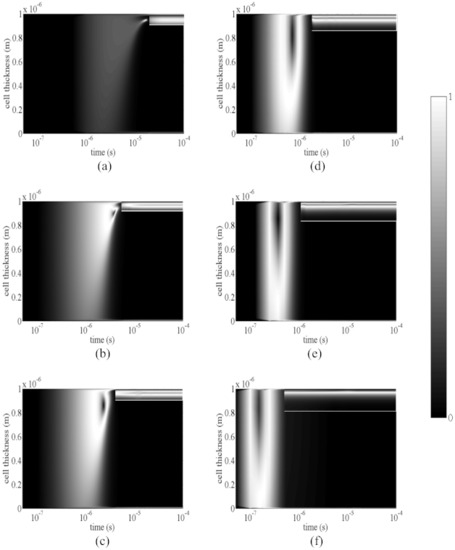
Figure 2.
Surface contour plots obtained at θL = 19° and θU = −3° for electric pulses with amplitudes of 15 V/μm (a), 22 V/μm (b), 25 V/μm (c), 40 V/μm (d), 60 V/μm (e), and 90 V/μm (f). The biaxiality is linearly mapped in a gray-level scale between black (zero biaxiality) and white (maximum biaxiality) colors. The cell thickness is represented on the vertical axis, while on the horizontal one, the solution’s evolution is reported in the 0 ms ≤ t ≤ 0.1 ms range in a logarithmic scale. In each panel, the inset shows the magnification not spatially scaled for the biaxiality within 15 nm under the upper boundary plate.
At t = 0 s, for each amplitude E of the AEF, the nematic molecules stayed in a planar configuration with respect to the surface and close to the upper boundary plate, while the bulk nematic texture had an asymmetric splayed configuration compatible with the prescribed boundary conditions. When applying a pulse E = 15 V/μm (Figure 2a) for t > 0 s, the director began to line up along the direction of the field. At the same time, close to the upper confining surface, the quasi-planar nematic texture was connected to the vertical one located in the bulk through a biaxial region of thickness comparable with ξb of about 20 nm. The nematic distortion tended toward the upper boundary plate, where it relaxed with the increasing biaxiality [23,24] locally replacing the starting uniaxial phase. Just underneath the upper surface, a bulk-order reconstruction occurred around t = 10 μs, characterized by the ring-like biaxial region surrounding a planar uniaxial state [12]. For t > 10 μs, a bent texture replaced the initial splayed one, and because of the imposed anchoring conditions, the biaxiality grew close to the upper boundary surface, while in the rest of the cell, the uniaxial order was restored. Near the upper surface in particular, the competition between the molecules lying in a quasi-planar configuration and the nematic texture aligned vertically along the field direction induced a strong distortion, which was relaxed by a growing biaxial wall [23] (see the inset of Figure 2a). When increasing the pulse amplitude, it is well known that the biaxial structures become faster [26], and at the same time, the bulk order reconstruction spreads progressively along the cell thickness, losing its cylindrical symmetry [27]. In the present case, as the competition between the quasi-planar texture and the vertical one became stronger close to the upper boundary plate, inside the surface biaxial wall, an order reconstruction transition occurred which lasted for the whole pulse duration (see the inset of Figure 2b–d), coexisting with the order reconstruction transition occurring in the bulk. At 60 V/μm for the applied field amplitude (Figure 2e), the surface-order reconstruction started decreasing, while at 90 V/μm (Figure 2f) it disappeared, and only the bulk order reconstruction was still present, which is delocalized along the z-direction [27]. Therefore, it seems that intense electric pulses applied to a π-cell with strong asymmetries allowed the coexistence of different switching mechanisms.
In Figure 3, we show the phase diagram obtained from monitoring the biaxiality inside the simulated domain for several (E,θU) pairs. Circles and squares mark the boundaries among the four regions where each texture obeys the same switching mechanisms: bulk switching (BS), surface switching (SS), bulk plus surface switching (BSS), or no switching (NS). In particular, the points in Figure 3 are given from the biaxiality computation performed for each value of the (E,θU) pair imposing θL = 19° and noting the resulting switching regime to which the texture was eventually attributed. The horizontal axis reports the amplitude of the electric pulse, while the vertical one represents the opposite of the anchoring angles θU. The data presented in [24] are well reproduced and marked with squares. As can be seen in Figure 3, most of the diagram concerns the textures for which bulk- and surface-order reconstruction coexist, while above E = 70 V/μm, only the bulk transition is present for whatever θU. The upper boundary delimiting BSS and BS switching exhibits a bi-lobed shape, suggesting that for points of the (E,θU) plane included under each lobed region, the corresponding textures may have behaved differently with regard to the relaxation of the nematic distortion along the cell thickness. In order to verify such an assumption, we identified in the (E,θU) plane the points marked by “x”. Since the electric field was applied along the e3 direction, we monitored the dynamics of the s3 eigenvalue, since it was sensitive to order variations along this direction [27] (see Figure 1). We also added (E = 42.5 V/μm, θU = −14°) and (E = 62 V/μm, θU = −14°), which were not drawn for plotting convenience. In Figure 4 and Figure 5, we show the s3 computations obtained for θU values of −4° (a), −6° (b), −9.5° (c), and −14° (d) for E = 42.5 V/μm and E = 62 V/μm, respectively. In both figures, time is reported in a logarithmic scale on the horizontal axis.
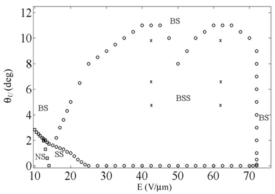
Figure 3.
Phase diagram of the biaxial order reconstruction obtained from imposing θL = 19°. The horizontal axis shows the amplitude E of the applied electric pulse, and the vertical one reports the opposite of the anchoring angle θU.
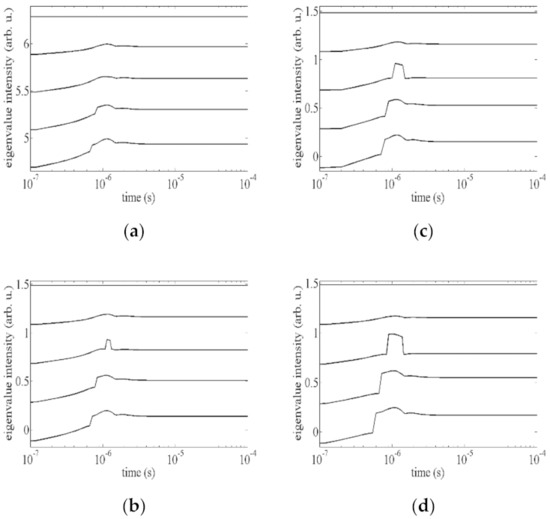
Figure 4.
Dynamical evolution of the s3 eigenvalue computed with an applied pulse E = 42.5 V/μm. In each panel, the plots refer to the first five mesh points starting from the upper boundary plate (top curve) for θU values of −4° (a), −6° (b), −9.5° (c), and −14° (d). On the horizontal axis, time is reported in a logarithmic scale.
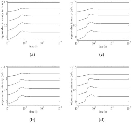
Figure 5.
Dynamical evolution of the s3 eigenvalue computed with an applied pulse E = 62 V/μm. In each panel, the plots refer to the first five mesh points starting from the upper boundary plate (top curve) for θU values of −4° (a), −6° (b), −9.5° (c), and −14° (d). On the horizontal axis, time is reported in a logarithmic scale.
Once E was fixed, for each θU value, the s3 dynamics were computed on the first five grid points, beginning from the upper boundary plate. The first curve from the top in each panel refers to the grid point located on the upper boundary surface, and it represents a constant s3, since along e3, the nematic order did not change, being prescribed by the fixed anchoring conditions. Under the upper boundary surface, instead, the nematic molecules began to align along the field direction, and the nematic distortion grew together with the biaxiality. For E = 42.5 V/μm and θU = −4° (Figure 4a), in the second and third curve under the top one, corresponding to the first two grid points under the upper plate, a smooth temporal evolution of s3 can be observed, a behavior characterizing biaxial phenomena as second-order transitions, since the nematic distortion relaxes through a wealth of biaxial states without any director rotation [27]. The fourth curve is characterized by a discontinuity highlighting a first-order transition. In fact, under the effect of the applied electric pulse, the director n reoriented along the e3 direction, and a predominant uniaxial order settled down. When imposing θU = −6° (Figure 4b), a sharp structure is visible during the dynamical evolution of s3 on the second grid point below the surface, which is superimposed to the smooth evolution. We interpreted such behavior as an attempt of the nematic director to reorient itself along the field direction which was suddenly aborted, meaning that the dynamical evolution of the biaxiality was mediated by a metastable uniaxial state. On the remaining two grid points, the s3 evolution shows a first-order transition superimposed to the smooth temporal evolution. For θU −9.5° and−14° (Figure 4c,d, respectively), nothing changed, except that all the features became sharper and faster, and the duration of the metastable state increased.
When increasing the pulse amplitude to E = 62 V/μm, for all the investigated θU values (see Figure 5a–d), the s3 temporal evolution was similar to the previous one at E = 42.5 V/μm, except that the metastable state disappeared, thus indicating that both the uniaxial and biaxial orders coexisted without the need for a metastable state to mediate the nematic order evolution.
The evolution of the s3 eigenvalue in Figure 4 displays evidence of a metastable state inside the nematic texture, located in a thin region below the upper boundary plate, whose existence depended on both the cell asymmetry (θU) and the AEF (E) but whose duration was determined by the θU value only. More generally, referring again to the phase diagram in Figure 3, it was possible to map nematic textures that, depending on the imposed electrical and mechanical stresses, relaxed the nematic distortion differently. In particular, two ranges of (E,θU) pairs were identified. There was a first one in which the nematic order showed a smooth and continuous biaxial evolution typical of a second-order transition, on which a first-order-like uniaxial transition was superimposed. Nematic textures falling in the second range of values at a lower electric distortion presented a qualitatively similar order evolution, but a nematic layer existed below the upper boundary surface, in which the superposition of the uniaxial transition was mediated by a uniaxial metastable state.
We believe such a result is worthy of further experimental investigations, as it might bring new and useful insights in the route of multi-stable device design [50,51].
Quite recent experiments have also been carried out to try to distinguish between surface- and bulk-order reconstruction phenomena [52,53]. One way was to investigate the electro-hydrodynamics of nematics and, in particular, the DSM1 and the DSM2 regimes. DSM1 and DSM2 behave very differently. DSM1 leaves the texture’s topology unchanged, while DSM2 generates textures that are topologically non-equivalent. Disclinations separate untwisted and π-twisted textures. Therefore, as in both cases, the initial state is quasi-planar and uniform, where DSM2 is characterized by irreversible order reconstruction phenomena, while DSM1 is only characterized by elastic reversible texture deformations. Unfortunately, as the surface extrapolation length and the biaxial coherence length in this system are comparable, the surface anchoring breaking is in the same order of the energy required for bulk-order reconstruction, and both surface and bulk phenomena can coexist for the transitions between untwisted and π-twisted textures. In DSM2, the static disclinations, separating the two topologically non-equivalent textures, are presumably formed by strong short-range fluctuations in the flow field due to the viscous coupling between the director and the flow field itself. In principle, it is possible to distinguish the anchoring breaking from the order reconstruction by spatially resolving the flow field at the scale of the biaxial coherence length and of the surface extrapolation length, which is 10 nm for both phenomena [53], but no decisive experiment has been performed up to now.
5. Conclusions
In this work, we presented a mathematical model with a numerical simulation to investigate the order tensor Q dynamical evolution for an NLC confined in a π-cell with strong asymmetries as well as strong electric distortions. For this purpose, we implemented the MMPDE numerical method using the FEM. Our simulations were consistent with previous computations, thus also confirming the validity of our numerical method in simulating notable distorted physical systems, as in the present case. Moreover, the peculiarity of the used technique revealed high sensitivity to distinguishing tiny features during the order dynamics of the studied system, allowing for building a phase diagram mapping the nematic regarding its switching properties, with computational savings with respect to the simulations performed using numerical techniques based on uniform discretizations. We considered several (E,θU) pairs, imposing strong anchoring conditions for the nematic molecules on both confining plates (with a fixed θL = 19° on the lower one), and then we carried out the simulations for several (E,θU) pairs, searching for the phase boundaries among nematic textures obeying different switching mechanisms. Textures undergoing the same switching mechanism were mapped in each of the four regions in which the (E,θU) plane was parted, while the phase diagram exhibits a bi-lobed region in which surface- and bulk-order reconstruction coexist. The Q-tensor dynamics show that the nematic textures mapped within the low-energy lobed region exhibited a switching mechanism that could be mediated by a metastable uniaxial state, as deduced from studying the evolution of the Q-tensor s3 eigenvalue. The study presented in this paper definitely indicates that strong distortions induced by electrical and mechanical stresses can be relaxed by order variations of the nematic texture up to admitting the coexistence of bulk- and surface-order reconstruction transitions.
The proposed problem involves characteristic lengths and times with large-scale differences, and although it is simplified and only in one dimension, it has almost all of the features of higher-dimensional real problems, making it a very useful model. Work is in progress to extend the computations in two-dimensional domains.
Author Contributions
All authors contributed equally to the manuscript. All authors have read and agreed to the published version of the manuscript.
Funding
Project DEMETRA: “Development of MatErial and TRAcking technologies for the safety of food”, PON ARS01_00401, Ministry of University and Research, MUR, Italy.
Institutional Review Board Statement
Not applicable.
Informed Consent Statement
Not applicable.
Data Availability Statement
Not applicable.
Conflicts of Interest
The authors declare no conflict of interest.
References
- Biscari, P.; Cesana, P. Ordering effects in electric splay Freedericksz transitions. Contin. Mech. Thermodyn. 2007, 19, 285–298. [Google Scholar] [CrossRef]
- De Gennes, P.G.; Prost, J. The Physics of Liquid Crystals, 2nd ed.; Clarendon Press: Oxford, UK, 1995. [Google Scholar]
- Tjipto, E.; Cadwell, K.D.; Quinn, J.F.; Johnston, A.P.R.; Abbott, N.L.; Caruso, F. Tailoring the interfaces between nematic liquid crystal emulsions and aqueous phases via layer-by-layer assembly. Nano Lett. 2006, 6, 2243–2248. [Google Scholar] [CrossRef] [PubMed]
- Aliev, F.; Basu, S. Relaxation of director reorientations in nanoconfined liquid crystal: Dynamic light scattering investigation. J. Non-Cryst. Solids 2006, 352, 4983–4987. [Google Scholar] [CrossRef]
- Schopohl, N.; Sluckin, T.J. Defect core structure in nematic liquid crystals. Phys. Rev. Lett. 1987, 59, 2582–2584. [Google Scholar] [CrossRef] [PubMed]
- Kleman, M.; Lavrentovich, O.D. Topological point defects in nematic liquid crystals. Philos. Mag. 2006, 86, 4117–4137. [Google Scholar] [CrossRef] [Green Version]
- Buscaglia, M.; Lombardo, G.; Cavalli, L.; Barberi, R.; Bellini, T. Elastic anisotropy at a glance: The optical signature of disclination lines. Soft Matter 2010, 6, 5434–5442. [Google Scholar] [CrossRef]
- Loudet, J.C.; Hanusse, P.; Poulin, P. Stokes drag on a sphere in a nematic liquid crystal. Science 2004, 306, 1525. [Google Scholar] [CrossRef]
- Smalyukh, I.I.; Lavrentovich, O.D.; Kuzmin, A.N.; Kachynski, A.V.; Prasad, P.N. Elasticity-mediated self-organization and colloidal interactions of solid spheres with tangential anchoring in a nematic liquid crystal. Phys. Rev. Lett. 2005, 95, 157801. [Google Scholar] [CrossRef] [PubMed] [Green Version]
- Muševič, I.; Škarabot, M.; Tkalec, U.; Ravnik, M.; Žumer, S. Two-dimensional nematic colloidal crystals self-assembled by topological defects. Science 2006, 313, 954–958. [Google Scholar] [CrossRef]
- De Gennes, P.G. Phenomenology of short-range-order effects in the isotropic phase of nematic materials. Phys. Lett. 1969, 30, 454–455. [Google Scholar] [CrossRef]
- Barberi, R.; Ciuchi, F.; Durand, G.; Iovane, M.; Sikharulidze, D.; Sonnet, A.; Virga, E.G. Electric field induced order reconstruction in a nematic cell. Eur. Phys. J. E 2004, 13, 61–71. [Google Scholar] [CrossRef] [PubMed]
- Barberi, R.; Ciuchi, F.; Lombardo, G.; Bartolino, R.; Durand, G.E. Time resolved experimental analysis of the electric field induced biaxial order reconstruction in nematics. Phys. Rev. Lett. 2004, 93, 137801. [Google Scholar] [CrossRef] [PubMed]
- Joly, S.; Dozov, I.; Martinot-Lagarde, P. Comment on “Time resolved experimental analysis of the electric field induced biaxial order reconstruction in nematics”. Phys. Rev. Lett. 2006, 96, 019801. [Google Scholar] [CrossRef]
- Lombardo, G.; Ayeb, H.; Ciuchi, F.; De Santo, M.P.; Barberi, R.; Bartolino, R.; Virga, E.G.; Durand, G.E. Inhomogeneous bulk nematic order reconstruction. Phys. Rev. E 2008, 77, 020702. [Google Scholar] [CrossRef]
- Lombardo, G.; Ayeb, H.; Barberi, R. Dynamical numerical model for nematic order reconstruction. Phys. Rev. E 2008, 77, 051708. [Google Scholar] [CrossRef]
- Carbone, G.; Lombardo, G.; Barberi, R.; Musevic, I.; Tkalec, U. Mechanically induced biaxial transition in a nanoconfined nematic liquid crystal with a topological defect. Phys. Rev. Lett. 2009, 103, 167801. [Google Scholar] [CrossRef]
- Qian, T.; Sheng, P. Biaxial ordering and field-induced configurational transition in nematic liquid crystals. Liq. Cryst. 1999, 26, 229–233. [Google Scholar] [CrossRef]
- Martinot-Lagarde, P.; Dreyfus-Lambez, H.; Dozov, I. Biaxial melting of the nematic order under a strong electric field. Phys. Rev. E 2003, 67, 051710. [Google Scholar] [CrossRef]
- Biscari, P.; Napoli, G.; Turzi, S. Bulk and surface biaxiality in nematic liquid crystals. Phys. Rev. E 2006, 74, 031708. [Google Scholar] [CrossRef] [PubMed] [Green Version]
- Ambrožič, M.; Kralj, S.; Virga, E.G. Defect-enhanced nematic surface order reconstruction. Phys. Rev. E 2007, 75, 031708. [Google Scholar] [CrossRef] [Green Version]
- Ayeb, H.; Lombardo, G.; Ciuchi, F.; Hamdi, R.; Gharbi, A.; Durand, G.E.; Barberi, R. Surface order reconstruction in nematics. Appl. Phys. Lett. 2010, 97, 104104. [Google Scholar] [CrossRef]
- Lombardo, G.; Amoddeo, A.; Hamdi, R.; Ayeb, H.; Barberi, R. Biaxial surface order dynamics in calamitic nematics. Eur. Phys. J. E 2012, 35, 9711–9716. [Google Scholar] [CrossRef] [PubMed] [Green Version]
- Amoddeo, A.; Barberi, R.; Lombardo, G. Surface and bulk contributions to nematic order reconstruction. Phys. Rev. E 2012, 85, 061705. [Google Scholar] [CrossRef] [PubMed]
- Amoddeo, A.; Barberi, R.; Lombardo, G. Moving mesh partial differential equations to describe nematic order dynamics. Comput. Math. Appl. 2010, 60, 2239–2252. [Google Scholar] [CrossRef] [Green Version]
- Amoddeo, A.; Barberi, R.; Lombardo, G. Electric field-induced fast nematic order dynamics. Liq. Cryst. 2011, 38, 93–103. [Google Scholar] [CrossRef]
- Amoddeo, A.; Barberi, R.; Lombardo, G. Nematic order and phase transition dynamics under intense electric fields. Liq. Cryst. 2013, 40, 799–809. [Google Scholar] [CrossRef]
- Tang, T. Moving mesh methods for computational fluid dynamics. Contemp. Math. 2005, 383, 141–173. [Google Scholar]
- Brimicombe, P.D.; Raynes, E.P. The influence of flow on symmetric and asymmetric splay state relaxations. Liq. Cryst. 2005, 32, 1273–1283. [Google Scholar] [CrossRef]
- Virga, E.G. Variational Theories for Liquid Crystals, 1st ed.; Chapman and Hall: London, UK, 1994. [Google Scholar]
- Sonnet, A.M.; Maffettone, P.; Virga, E.G. Continuum theory for nematic liquid crystals with tensorial order. J. Non-Newton. Fluid Mech. 2004, 119, 51–59. [Google Scholar] [CrossRef]
- Sonnet, A.M.; Virga, E.G. Dynamics of dissipative ordered fluids. Phys. Rev. E 2001, 64, 031705. [Google Scholar] [CrossRef]
- Ambrožič, M.; Bisi, F.; Virga, E.G. Director reorientation and order reconstruction: Competing mechanisms in a nematic cell. Contin. Mech. Thermodyn. 2008, 20, 193–218. [Google Scholar] [CrossRef]
- Anderson, J.; Watson, P.; Bos, P. LC3D: Liquid Crystal Display 3-D Directory Simulator, Software and Technology Guide; Artech House: Boston, MA, USA, 2001. [Google Scholar]
- Alexe-Ionescu, A. Flexoelectric polarization and 2nd order elasticity for nematic liquid crystals. Phys. Lett. A 1993, 180, 456–460. [Google Scholar] [CrossRef]
- Zienkiewicz, O.; Taylor, R. The Finite Element Method; Butterworth–Heinemann: Oxford, UK, 2002. [Google Scholar]
- Beckett, G.; Mackenzie, J.A.; Ramage, A.; Sloan, D.M. On the numerical solution of one-dimensional PDEs using adaptive methods based on equidistribution. J. Comput. Phys. 2001, 167, 372–392. [Google Scholar] [CrossRef]
- De Boor, C. Good approximation by splines with variable knots II. In Numerical Solution of Differential Equations, Proceedings of the Conference on the Numerical Solution of Differential Equations, Dundee, UK, 3–6 July 1973; Watson, G.A., Ed.; Springer: Berlin/Heidelberg, Germany, 1974; pp. 12–20. [Google Scholar]
- Pereyra, V.; Sewell, E.G. Mesh selection for discrete solution of boundary problems in ordinary differential equations. Numer. Math. 1974, 23, 261–268. [Google Scholar] [CrossRef]
- Russell, R.D.; Christiansen, J. Adaptive mesh selection strategies for boundary value problems. SIAM J. Numer. Anal. 1978, 15, 59–80. [Google Scholar] [CrossRef]
- White, A.B. On selection of equidistributing meshes for two-point boundary-value problems. SIAM J. Numer. Anal. 1979, 16, 472–502. [Google Scholar] [CrossRef]
- Ramage, A.; Newton, C.J.P. Adaptive solution of a one-dimensional order reconstruction problem in Q-tensor theory of liquid crystals. Liq. Cryst. 2007, 34, 479–487. [Google Scholar] [CrossRef]
- Beckett, G.; Mackenzie, J.A. Convergence analysis of finite difference approximations on equidistributed grids to a singularly perturbed boundary value problem. Appl. Numer. Math. 2000, 35, 87–109. [Google Scholar] [CrossRef]
- Huang, W. Practical aspects of formulation and solution of moving mesh partial differential equations. J. Comput. Phys. 2001, 171, 753–775. [Google Scholar] [CrossRef] [Green Version]
- Huang, W.; Ren, Y.; Russell, R.D. Moving mesh partial differential equations (MMPDEs) based upon the equidistribution principle. SIAM J. Numer. Anal. 1994, 31, 709–730. [Google Scholar] [CrossRef]
- Anderson, J.; Titus, C.; Watson, P.; Bos, P. Significant speed and stability increases in multi-dimensional director simulations. SID Dig. 2000, 31, 906–909. [Google Scholar] [CrossRef]
- Ratna, B.R.; Shashidhar, R. Dielectric studies on liquid crystals of strong positive dielectric anisotropy. Mol. Cryst. Liq. Cryst. 1977, 42, 113–125. [Google Scholar] [CrossRef]
- Amoddeo, A. Nematodynamics modelling under extreme mechanical and electric stresses. J. Phys. Conf. Ser. 2015, 574, 012102. [Google Scholar] [CrossRef]
- Amoddeo, A. Concurrence of bulk and surface order reconstruction to the relaxation of frustrated nematics. J. Phys. Conf. Ser. 2016, 738, 012089. [Google Scholar] [CrossRef] [Green Version]
- Klemencic, E.; Kurioz, P.; Kralj, S.; Repnik, R. Topological defect enabled formation of nematic domains. Liq. Cryst. 2020, 47, 618–625. [Google Scholar] [CrossRef]
- Wu, J.; Ma, H.; Chen, S.; Zhou, X.; Zhang, Z. Study on concentric configuration of nematic liquid crystal droplet by Landau-de Gennes theory. Liq. Cryst. 2020, 47, 1698–1707. [Google Scholar] [CrossRef]
- Pucci, G.; Lysenko, D.; Provenzano, C.; Reznikov, Y.; Cipparrone, G.; Barberi, R. Patterns of electro-convection in planar-periodic nematic cells. Liq. Cryst. 2016, 43, 216–221. [Google Scholar] [CrossRef]
- Pucci, G.; Carbone, F.; Lombardo, G.; Versace, C.; Barberi, R. Topologically non-equivalent textures generated by the nematic electrohydrodynamic. Liq. Cryst. 2019, 46, 649–654. [Google Scholar] [CrossRef]
Publisher’s Note: MDPI stays neutral with regard to jurisdictional claims in published maps and institutional affiliations. |
© 2021 by the authors. Licensee MDPI, Basel, Switzerland. This article is an open access article distributed under the terms and conditions of the Creative Commons Attribution (CC BY) license (https://creativecommons.org/licenses/by/4.0/).