
Partial Covering of a Circle by 6 and 7 Congruent Circles

Abstract
1. Introduction
2. Method
3. Optimal Packings of Six Circles
4. Coverings by Six Circles
5. Equilibrium Paths in the Case of Six Circles
5.1. Equilibrium Path Starting from the Packing of Symmetry
5.1.1. The Branch of Symmetry
5.1.2. The Branch of Symmetry
5.1.3. The Branch of (Pumpkin) Symmetry
5.1.4. The Branch of (Rugby Ball) Symmetry
5.1.5. The Branch of Symmetry
5.1.6. The Branch of Symmetry
5.1.7. The Branch of Symmetry
5.2. Equilibrium Path Starting from the Packing of Symmetry
5.2.1. The Branch of Symmetry
5.2.2. The Segment
5.2.3. The Segment
5.2.4. The Branch of Symmetry
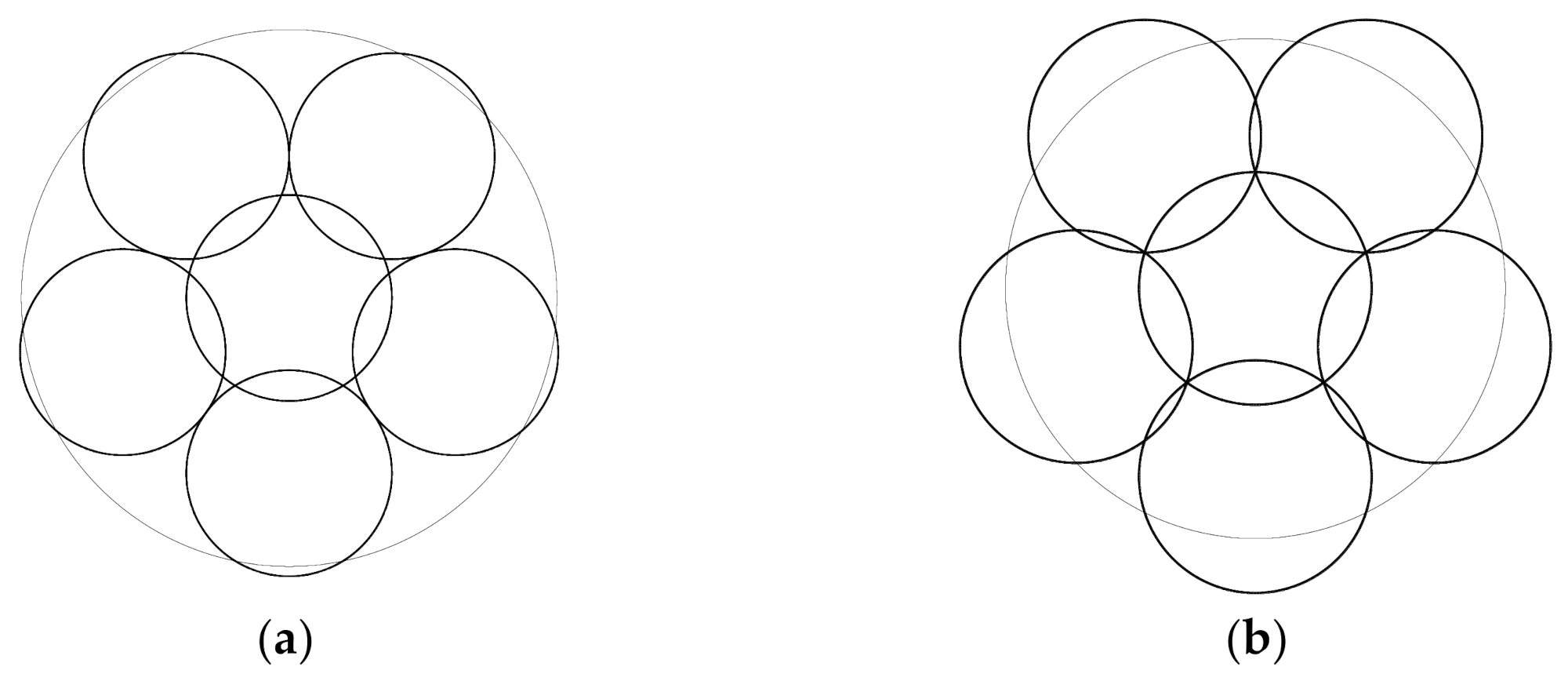
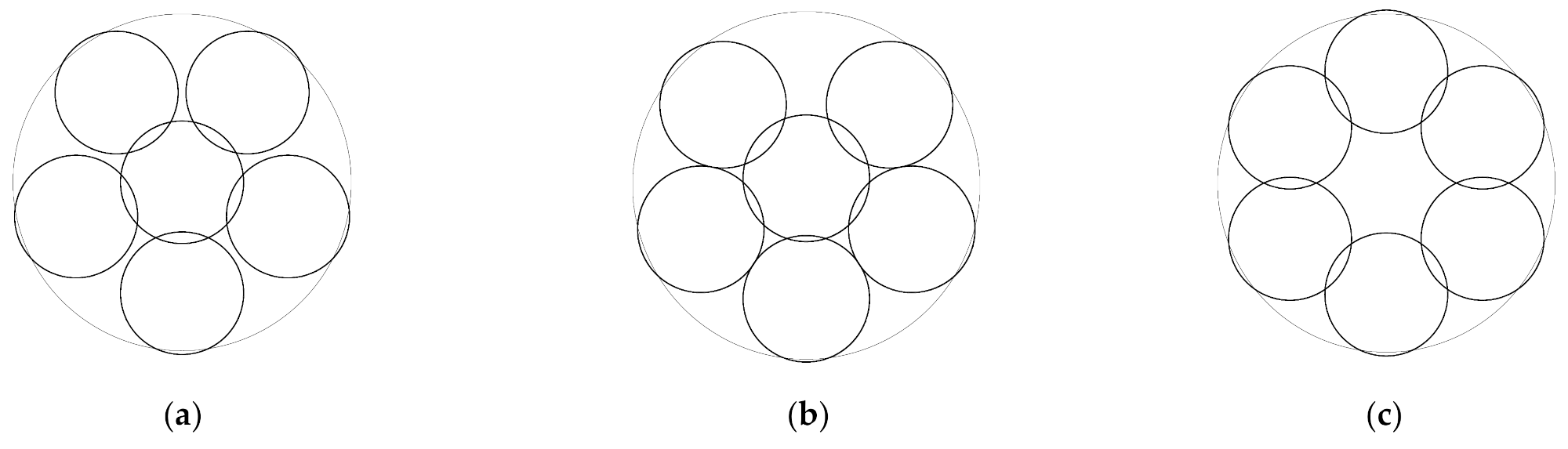
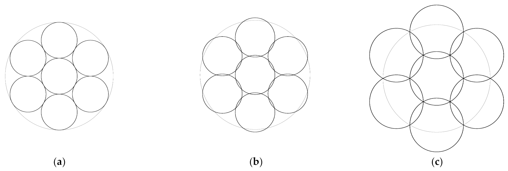
- (a)
- symmetry discussed in Section 5.2.1 (there is not even a local optimum, coverage: 0.7643588212),
- (b)
- symmetry (local optimum, coverage: 0.7651570086),
- (c)
- symmetry discussed in Section 5.1.1 (local optimum, coverage: 0.7582353854).
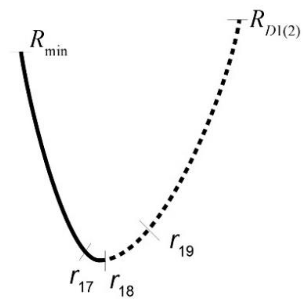
- (i)
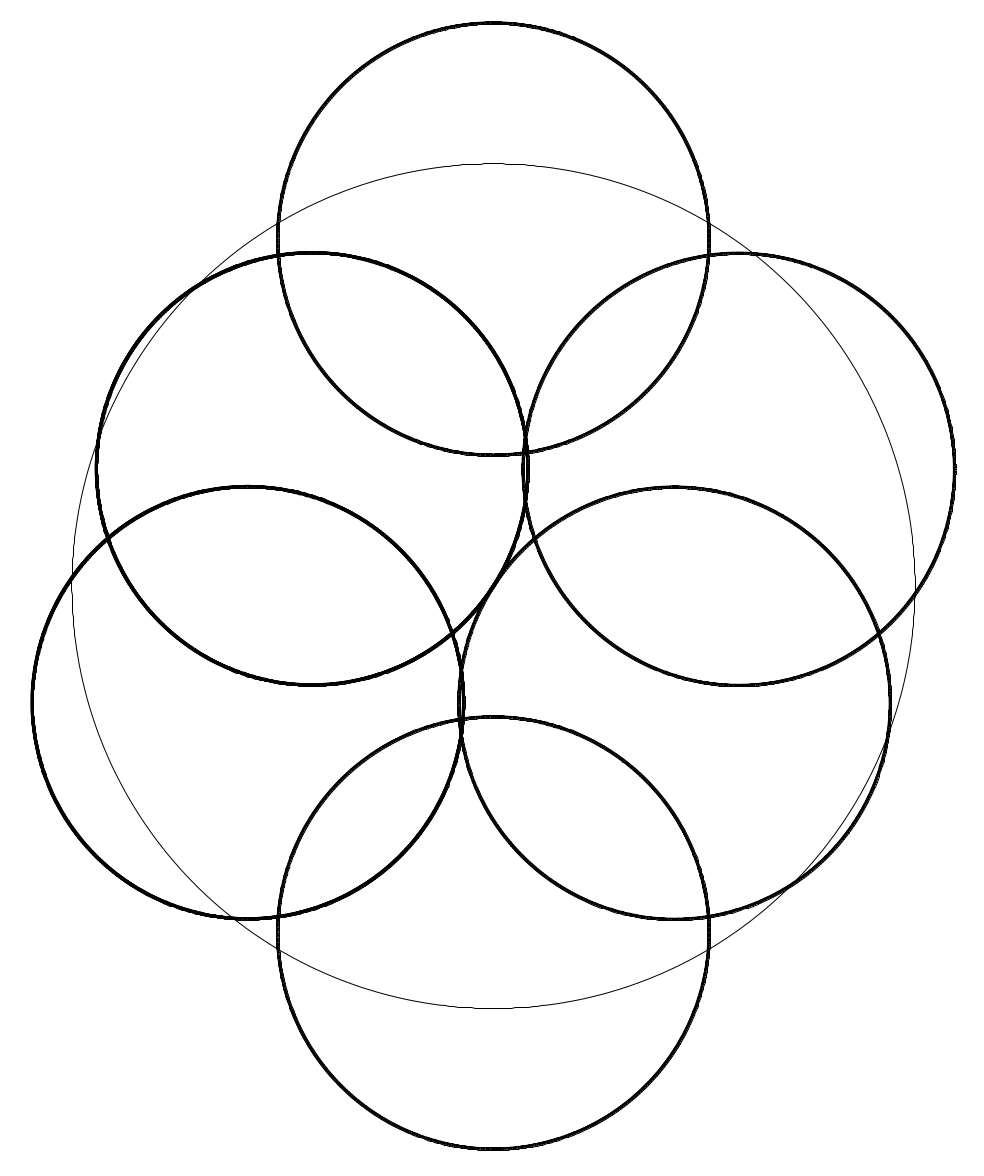
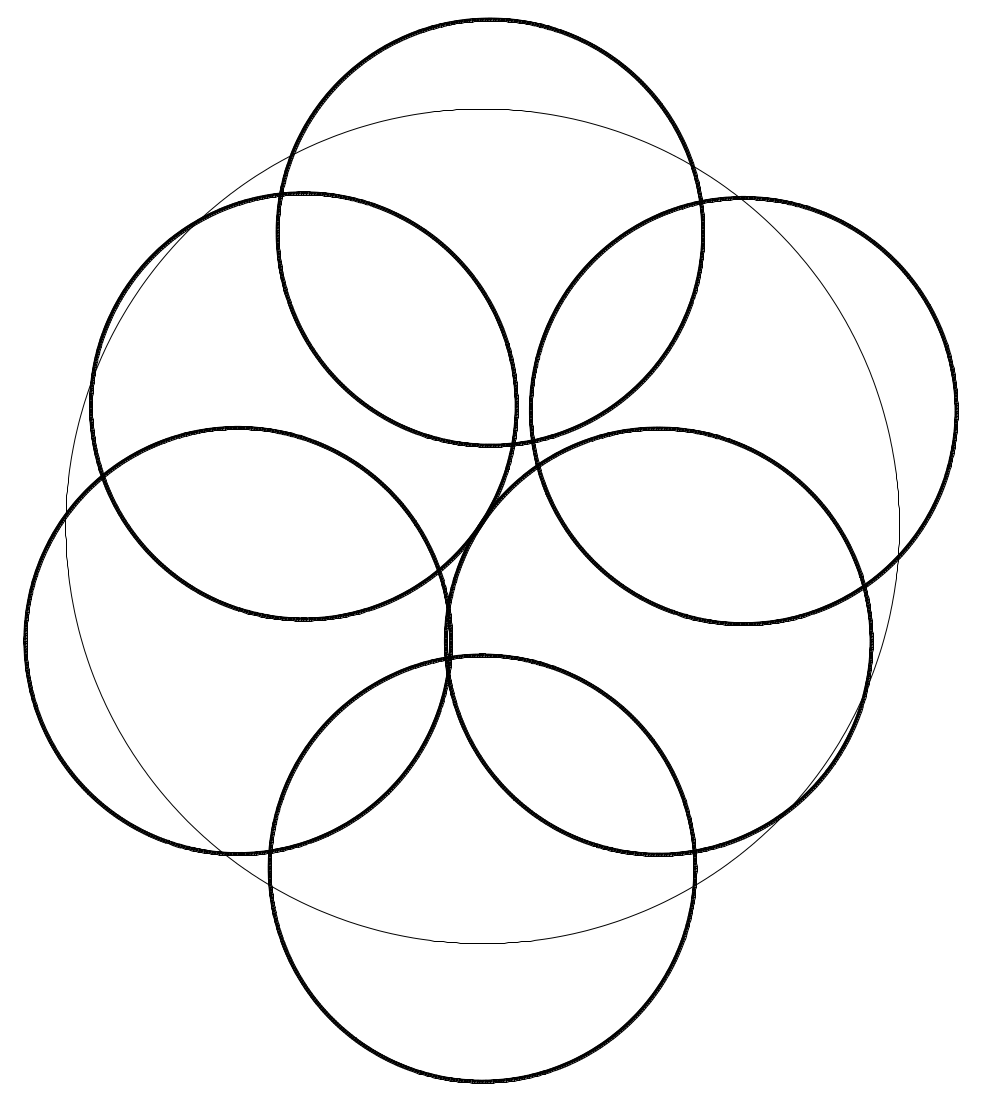
- In the arrangement shown in Figure 14b, the gap visible at the top gradually decreases,
- (ii)
- The displacement of the middle circle increases, then begins to decrease, and finally it becomes zero at the radius , that is, the arrangement of symmetry passes into an arrangement of symmetry.
5.3. Equilibrium Path Starting from the Optimal Covering
6. Summary of the Results Concerning Six Circles
- The equilibrium paths form three different systems that are unconnected to each other (systems starting from the packings of and symmetries and the optimal covering);
- For the branches associated with the equilibrium path of the symmetry arrangement, the product of the number of cycles and the number of branches, if there is an axis of symmetry (type ), then six, otherwise (type ), 12;
- The equilibrium path corresponding to the symmetry arrangement has two strongly degenerate segments, at each point of which the equilibrium path bifurcates in an infinite number of directions, i.e., in the neighbourhood of these segments the equilibrium positions form a three-dimensional set.
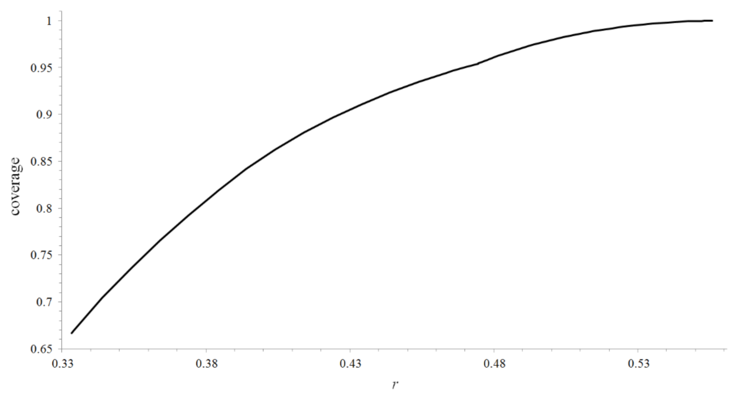
- in the interval by the arrangement corresponding to ,
- in the interval by the arrangement corresponding to ,
- in the interval (0.47449, 0.54715) by the arrangement corresponding to ,
- in the interval by the arrangement corresponding to
7. Optimal Arrangements of 7 Circles
8. Conclusions
- Are not connected to each other;
- At each path, there is a branch corresponding to a locally optimal arrangement;
- The arrangements corresponding to the global optimum are divided between these three independent paths;
- Here, too, the bifurcation types experienced for n = 5 occur, in fact;
- Here were segments where the stiffness matrix was singular at each point of certain segments of the equilibrium path, so that the equilibrium path degenerated into equilibrium body.
Author Contributions
Funding
Institutional Review Board Statement
Informed Consent Statement
Data Availability Statement
Acknowledgments
Conflicts of Interest
References
- Zahn, C.T. Black box maximization of circular coverage. J. Res. Nat. Bur. Stand. B 1962, 66, 181–216. [Google Scholar] [CrossRef]
- Hangody, L.; Feczkó, P.; Bartha, L.; Bodó, G.; Kish, G. Mosaicplasty for the treatment of articular defects of the knee and ankle. Clic. Orthop. Relat. Res. 2001, 391, S328–S336. [Google Scholar] [CrossRef] [PubMed]
- Graham, R.L. Sets of points with given minimum separations (Solutions to Problem E 1921). Amer. Math. Mon. 1968, 75, 192–193. [Google Scholar]
- Pirl, U. Der Mindestabstand von n in der Einheitskreisscheibe gelagenen Punkten. Math. Nachr. 1969, 40, 111–124. [Google Scholar] [CrossRef]
- Melissen, H. Densest packing of eleven congruent circles in a circle. Geom. Dedicata. 1994, 50, 15–25. [Google Scholar] [CrossRef]
- Fodor, F. The densest packing of 19 congruent circles in a circle. Geom. Dedicata. 1999, 74, 139–145. [Google Scholar] [CrossRef]
- Fodor, F. The densest packing of 12 congruent circles in a circle. Beiträge Algebra Geom. 2000, 41, 401–409. [Google Scholar]
- Fodor, F. The densest packing of 13 congruent circles in a circle. Beiträge Algebra Geom. 2003, 44, 431–440. [Google Scholar]
- Fodor, F. Packing of 14 congruent circles in a circle. Stud. Univ. Žilina Math. Ser. 2003, 16, 25–34. [Google Scholar]
- Bezdek, K. Optimal Covering of Circles; Thesis: Budapest, Hungary, 1979. (In Hungarian) [Google Scholar]
- Bezdek, K. Über einige Kreisüberdeckungen. Beiträge Algebra Geom. 1983, 14, 7–13. [Google Scholar]
- Fejes Tóth, G. Thinnest covering of a circle by eight, nine, or ten congruent circles. In Combinatorial and Computational Geometry; Mathematical Sciences Research Institute Publications; Goodman, J.E., Pach, J., Welzl, E., Eds.; Cambridge University Press: Cambridge, UK, 2005; Volume 52, pp. 361–376. [Google Scholar]
- Graham, R.L.; Lubachevsky, B.D.; Nurmela, K.J.; Östergård, P.R.L. Dense packings of congruent circles in a circle. Discrete Math. 1998, 181, 139–154. [Google Scholar] [CrossRef]
- Nurmela, K.J. Covering a Circle by Congruent Circular Discs; Department of Computer Science and Engineering, Helsinki University of Technology: Espoo, Finland, 1998; preprint. [Google Scholar]
- Szalkai, B. Optimal cover of a disk with three smaller congruent disks. Adv. Geom. 2016, 16, 465–476. [Google Scholar] [CrossRef]
- Gáspár, Z.; Tarnai, T.; Hincz, K. Partial covering of the unit circle by four equal circles. Annales Univ. Sci. Budapest. 2017, 60, 137–144. [Google Scholar]
- Gáspár, Z.; Tarnai, T.; Hincz, K. Partial covering of a circle by equal circles, Part II: The case of 5 circles. J. Comput. Geom. 2014, 5, 126–149. [Google Scholar]
- Coxeter, H.S.M. Introduction to Geometry; Wiley: New York, NY, USA, 1961. [Google Scholar]
- Weil, H. Symmetry; Princeton University Press: Princeton, NJ, USA, 1952. [Google Scholar]
- Poston, T.; Stewart, I. Catastrophe Theory and Its Applications; Pitman: London, UK, 1978. [Google Scholar]
- Fejes Tóth, L. Über die Abschetzung des kürzesten Abstandes zweier Punkte eines auf einer Kugelfläche liegenden Punktsystems. Jber. Dtsch. Math.-Ver. 1943, 53, 66–68. [Google Scholar]
- Schütte, K.; van der Waerden, B.L. Auf welcher Kugel haben 5, 6, 7, 8 oder 9 Punkte mit Mindestabstand ein Platz? Math. Annln. 1951, 123, 96–124. [Google Scholar] [CrossRef]
- Danzer, L. Endliche Punktmengen auf der 2-Sphäre mit möglichst grossem Minimalabstand; Habilitationschrift: Universität Göttingen: Göttingen, Germany, 1963. [Google Scholar]
- Musin, O.R.; Tarasov, A.S. Enumeration of irreducible contact graphs on the sphere. J. Math. Sci. 2014, 203, 837–850. [Google Scholar] [CrossRef][Green Version]
- Musin, O.R.; Tarasov, A.S. The Tammes problem for N = 14. Experimental Math. 2015, 24, 460–468. [Google Scholar] [CrossRef]
- Robinson, R.M. Arrangement of 24 points on a sphere. Math. Annln. 1961, 144, 17–48. [Google Scholar] [CrossRef]
- Fejes Tóth, L. On covering the spherical surface with equal spherical caps. Matematikai Fiz. Lapok 1943, 50, 40–46. (In Hungarian) [Google Scholar]
- Schütte, K. Überdeckung der Kugel mit höchstens acht Kreisen. Math. Annln 1955, 129, 181–186. [Google Scholar] [CrossRef]
- Wimmer, L. Covering the sphere with equal circles. Discrete Comp. Geom. 2017, 57, 763–781. [Google Scholar] [CrossRef]
- Fejes Tóth, G. Kreisüberdeckungen der Sphäre. Studia Sci. Math. Hungar. 1969, 4, 225–247. [Google Scholar]
- Sloane, N.J.A.; Hardin, R.H.; Smith, W.D. Spherical Codes. Available online: NeilSloane.com/packings/ (accessed on 7 October 2021).
- Hardin, R.H.; Sloane, N.J.A.; Smith, W.D. Spherical Coverings. Available online: NeilSloane.com/coverings/ (accessed on 7 October 2021).
- Fejes Tóth, L. Regular Figures; Pergamon; Macmillan: New York, NY, USA, 1964. [Google Scholar]
- Fejes Tóth, L. Perfect distribution of points on a sphere. Periodica Math. Hungar. 1971, 1, 25–33. [Google Scholar] [CrossRef]
- Fowler, P.W.; Tarnai, T. Transition from spherical circle packing to covering: Geometrical analogues of chemical isomerization. Proc. R. Soc. Lond. Ser. A Math. Phys. Eng. Sci. 1996, 452, 2043–2064. [Google Scholar]
- Fowler, P.W.; Tarnai, T. Transition from circle packing to covering on a sphere: The odd case of 13 circles. Proc. R. Soc. Lond. Ser. A Math. Phys. Eng. Sci. 1999, 455, 4131–4143. [Google Scholar] [CrossRef]
- Gáspár, Z.; Tarnai, T.; Hincz, K. Partial covering of a circle by equal circles, Part I: The mechanical models. J. Comput. Geom. 2014, 5, 104–125. [Google Scholar]
- Csikós, B. On the volume of the union of balls. Discrete Comput. Geom. 1998, 20, 449–461. [Google Scholar] [CrossRef]
- Connelly, R. Maximizing the Area of Unions and Intersections of Discs. Lecture at the Discrete and Convex Geometry Workshop; Alfréd Rényi Institute of Mathematics: Budapest, Hungary, 2008. [Google Scholar]
- Pacioli, L. Summa de Arithmetica, Geometria, Proportioni et Proportionalita; Paganius de Paganinis: Venezia, Italy, 1494. [Google Scholar]


| Coverage | Figure Number | |||||
|---|---|---|---|---|---|---|
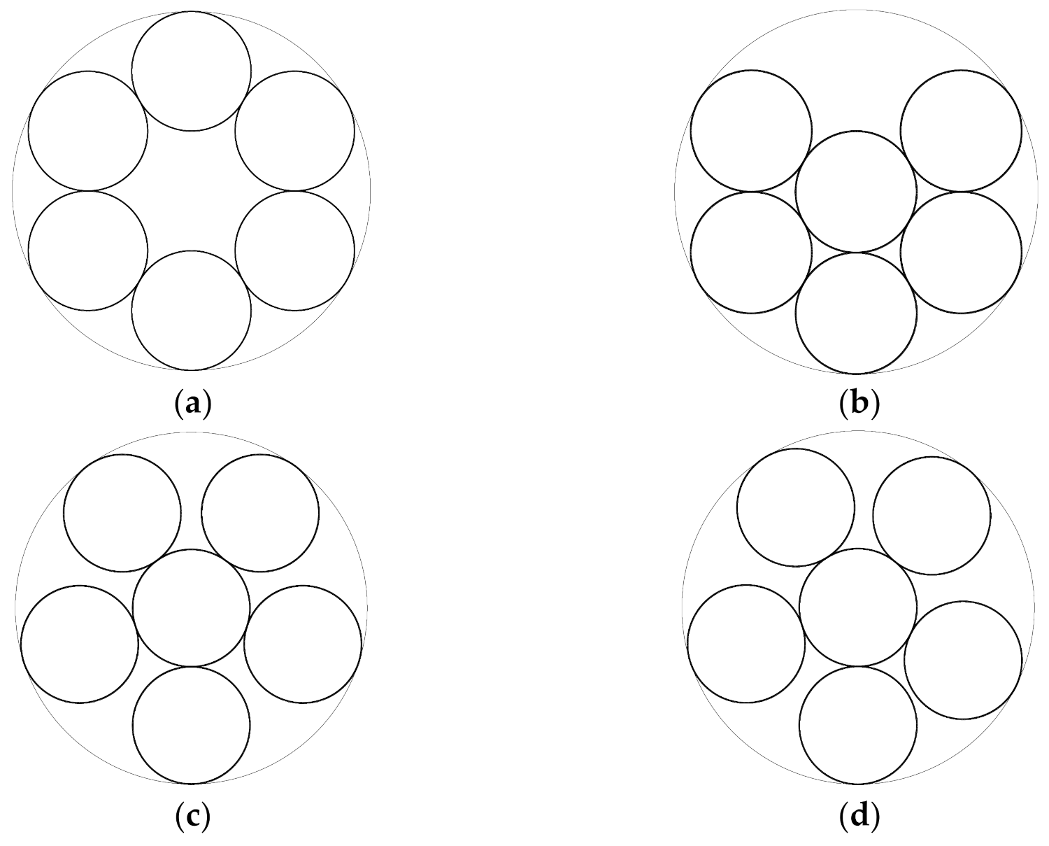
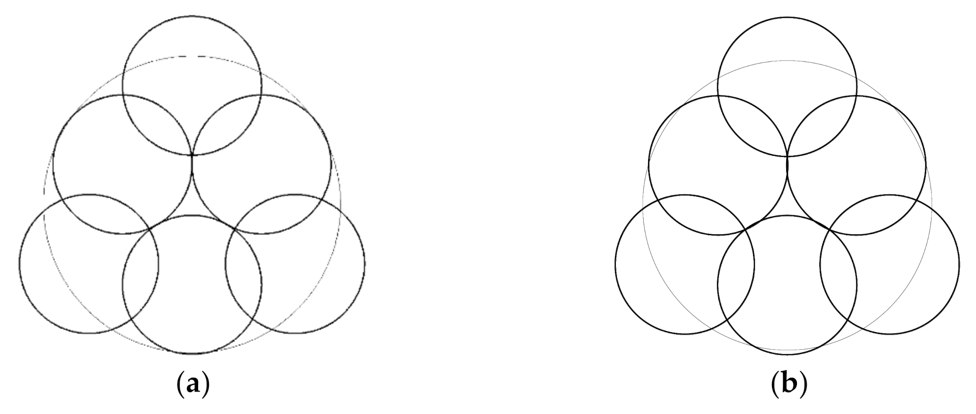
| 0.3333333333 | 1,6 | 0 | 0.6666666667 | 0.6666666667 | 2a | |
| 2–5 | 0.5773502692 | 0.3333333333 | ||||
| 0.3333333333 | 1 | 0 | 0 | 0.6666666667 | 2b | |
| 2–5 | 0.5773502692 | 0.3333333333 | ||||
| 6 | 0 | −0.6666666667 | ||||
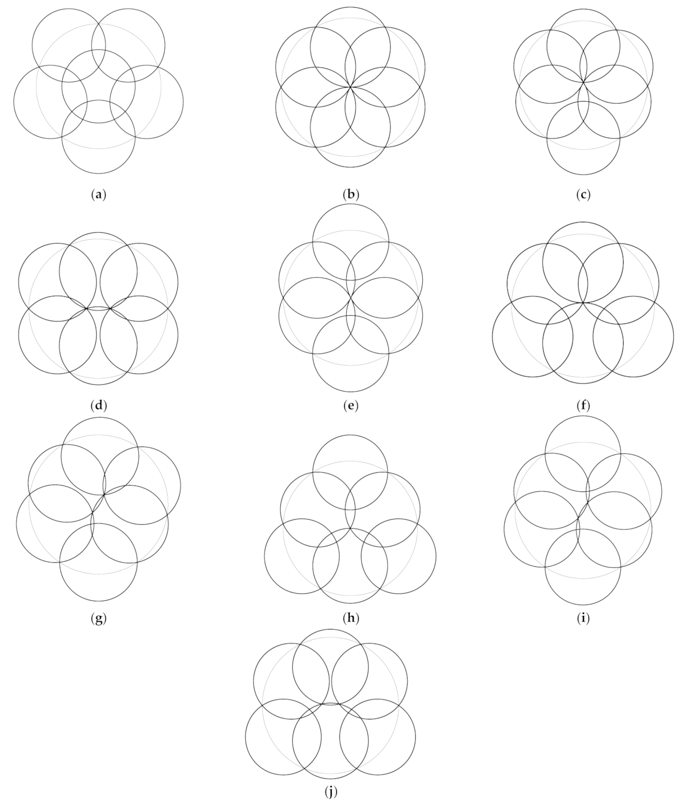
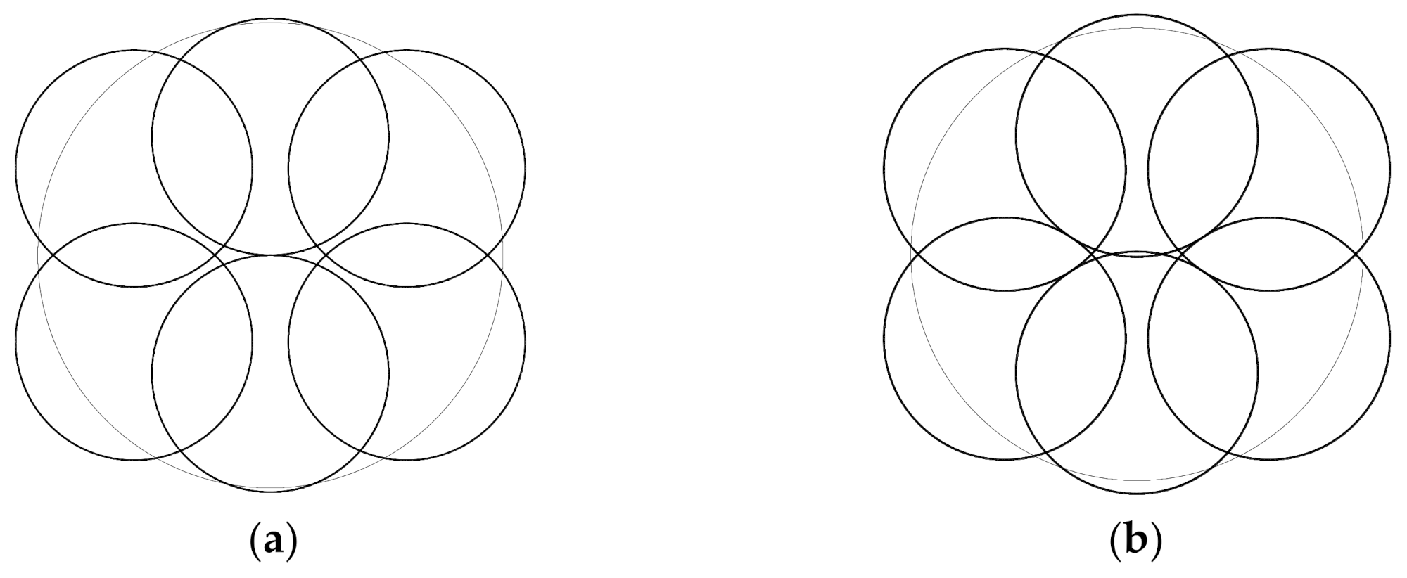
| 0.5877852523 | 1 | 0 | 0 | 1 | 3a | |
| 2,3 | 0.4755285518 | 0.6545089014 | ||||
| 4,5 | 0.7694213635 | −0.2500001557 | ||||
| 6 | 0 | −0.8090171626 | ||||
| 0.5773502692 | 1,6 | 0 | 0.5773502691 | 1 | 3b | |
| 2–5 | 0.5 | 0.2886751345 | ||||
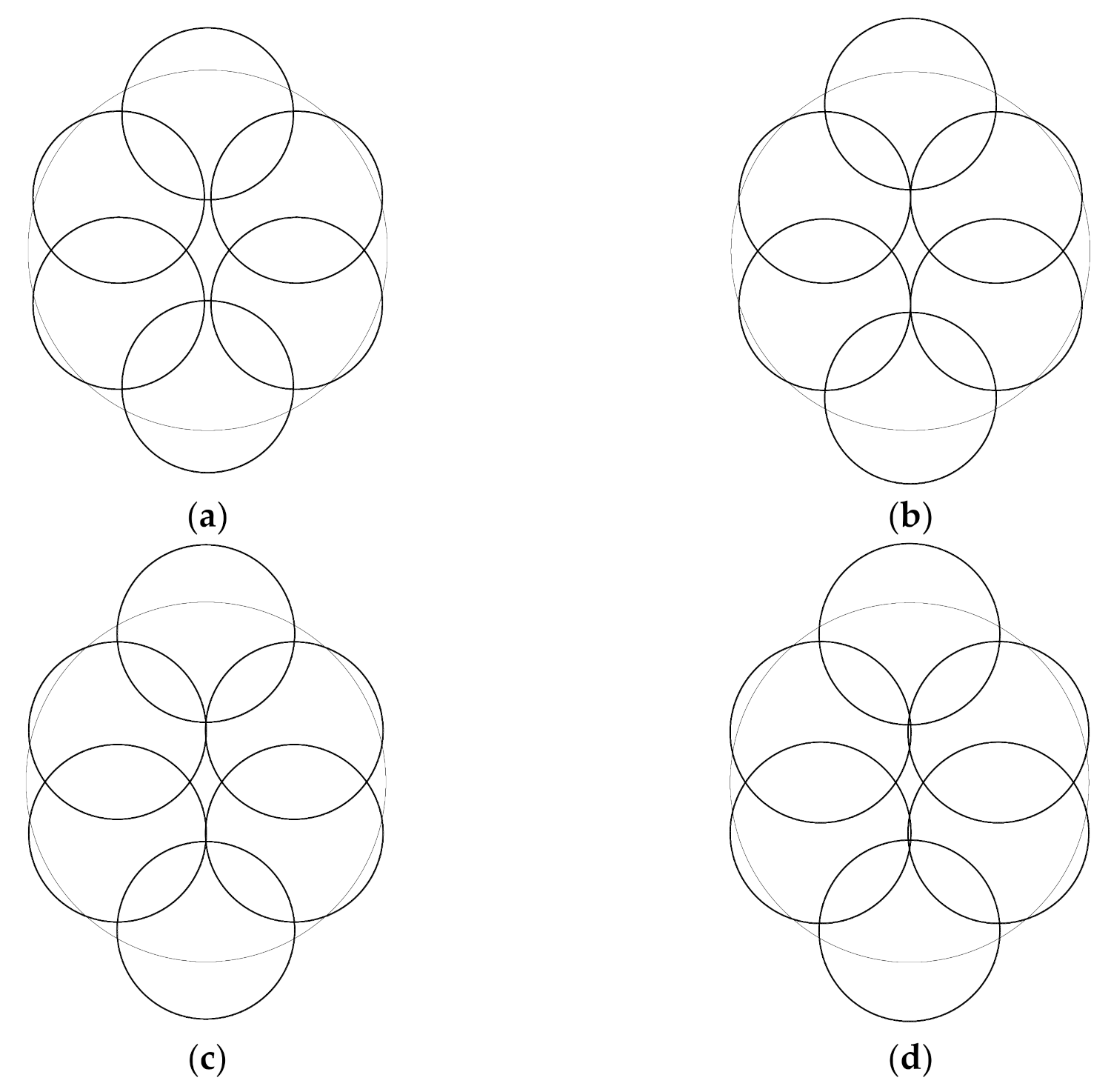
| 0.5701976646 | 1 | 0 | 0.6127107125 | 1 | 3c | |
| 2,4 | 0.5151767615 | 0.2868862895 | ||||
| 3,5 | 0.4847337508 | −0.2577511152 | ||||
| 6 | 0 | −0.8215075308 | ||||
| 0.5600968657 | 1,6 | 0 | 0.5331709364 | 1 | 3d | |
| 2–5 | 0.5857864376 | 0.3770087846 | ||||
| 0.5651977174 | 1,6 | 0 | 0.8249554777 | 1 | 3e | |
| 2–5 | 0.5 | 0.2635307567 | ||||
| 0.5635253276 | 1 | 0 | 0.6026560414 | 1 | 3f | |
| 2,4 | 0.4974006067 | 0.3039956419 | ||||
| 3,5 | 0.7035513014 | −0.4329604734 | ||||
| 6 | 0 | −0.5243946138 | ||||
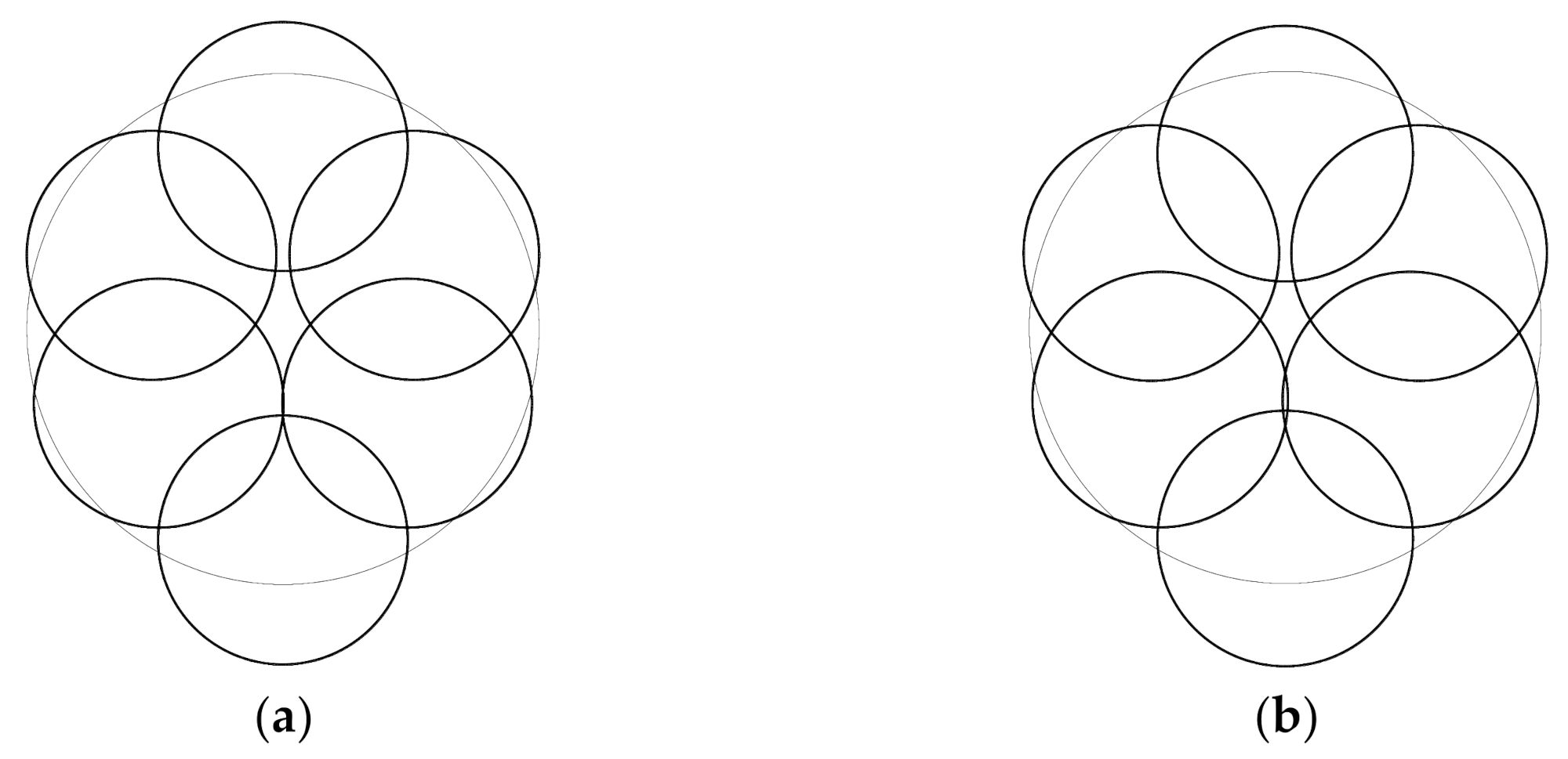
| 0.5583182642 | 1 | 0.0213089294 | 0.6939095997 | 1 | 3g | |
| 2 | 0.6222895494 | 0.2706667445 | ||||
| 3 | 0.4460901879 | −0.2827044247 | ||||
| 4 | −0.4535669631 | 0.3037046943 | ||||
| 5 | −0.6229495950 | −0.2750620915 | ||||
| 6 | 0 | −0.8296268534 | ||||
| 0.5570157181 | 1 | 0 | 0.8305019505 | 1 | 3h | |
| 2,3 | 0.4823897622 | 0.2785078591 | ||||
| 4,5 | 0.7192357870 | −0.4152509752 | ||||
| 6 | 0 | −0.5570157181 | ||||
| 0.5565264632 | 1,6 | 0 | 0.8308298838 | 1 | 3i | |
| 2,5 | 0.6031630184 | 0.2762609196 | ||||
| 3,4 | 0.4600218720 | 0.2827344832 | ||||
| 0.5559052114 | 1 | 0 | 0.5617874316 | 1 | 3j | |
| 2,3 | 0.5725482556 | 0.3549534480 | ||||
| 4,5 | 0.6907587242 | −0.4624086729 | ||||
| 6 | 0 | −0.5200412247 | ||||
| Coverage | Figure Number | |||||
|---|---|---|---|---|---|---|
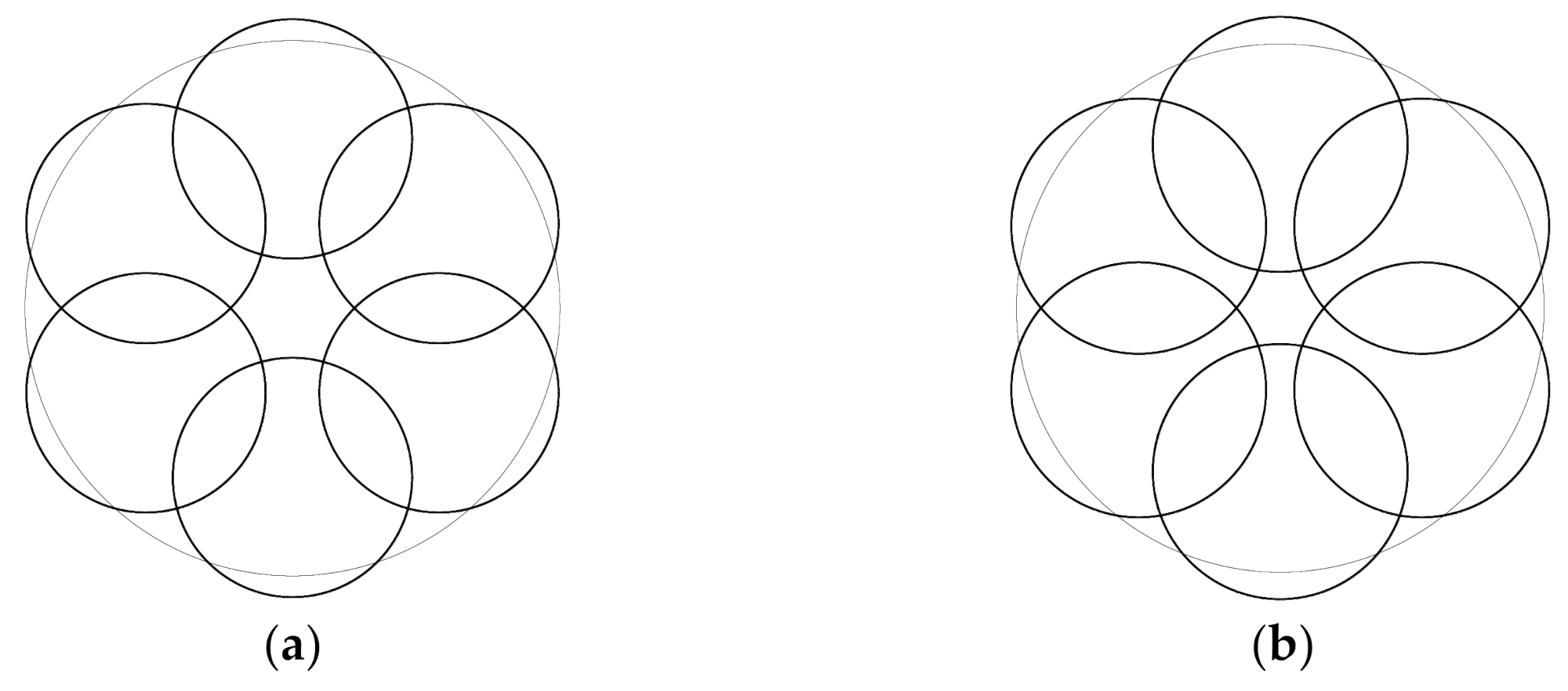
| 0.4472135955 | 1,6 | 0 | 0.6324555320 | 0.9144982941 | 5a | |
| 2–5 | 0.5477225575 | 0.3162277660 | ||||
| 0.4827200179 | 1,6 | 0 | 0.6192662531 | 0.9551984579 | 5b | |
| 2–5 | 0.5363003069 | 0.3096331265 | ||||
| 0.4681235977 | 1 | 0 | 0.8004294056 | 0.9452009602 | 6a | |
| 2,3 | 0.4681235977 | 0.2702712851 | ||||
| 4,5 | 0.6931921992 | −0.4002147028 | ||||
| 6 | 0 | −0.5405425703 | ||||
| 0.4810603043 | 1 | 0 | 0.8176825088 | 0.9621897743 | 6b | |
| 2,3 | 0.4771598040 | 0.2754883414 | ||||
| 4,5 | 0.7081338249 | −0.4088412544 | ||||
| 6 | 0 | −0.5509766826 | ||||
| 0.5089334763 | 1,6 | 0 | 0.5089334763 | 0.9791020416 | 7a | |
| 2–5 | 0.5860490667 | 0.3721826799 | ||||
| 0.5349571702 | 1,6 | 0 | 0.5233712202 | 0.9952931802 | 7b | |
| 2–5 | 0.5840892239 | 0.3730418956 | ||||
| 0.4771231753 | 1,6 | 0 | 0.7568326369 | 0.9495539652 | 8a | |
| 2–5 | 0.4952596676 | 0.2945440486 | ||||
| 0,4777166212 | 1,6 | 0 | 0,8196347452 | 0.9502891973 | 8b | |
| 2–5 | 0,4777166212 | 0,2987485232 | ||||
| 0.4932700700 | 1,6 | 0 | 0.8248914501 | 0.9676505985 | 8c | |
| 2–5 | 0.4911006728 | 0.2854100068 | ||||
| 0.5039429803 | 1,6 | 0 | 0.8242468715 | 0.9769519459 | 8d | |
| 2–5 | 0.4957014235 | 0.2799112855 | ||||
| 0.48744564 | 1 | 0 | 0.7142214866 | 0.9612059828 | 9a | |
| 2,3 | 0.5129878451 | 0.2883233530 | ||||
| 4,5 | 0.4850429130 | −0.2903674287 | ||||
| 6 | 0 | −0.8261517093 | ||||
| 0.4990334240 | 1 | 0 | 0.6785170299 | 0.9717499000 | 9b | |
| 2,3 | 0.5228790959 | 0.2905235730 | ||||
| 4,5 | 0.4884398843 | −0.2816791405 | ||||
| 6 | 0 | −0.8241558231 | ||||
| 0.5116675879 | 1,6 | 0 | 0.8214382601 | 0.9831869003 | 10 | |
| 2,5 | 0.5822443882 | 0.2762544436 | ||||
| 3,4 | 0.4298786085 | 0.2775033377 | ||||
| 0.5105307 | 1 | 0.0190552071 | 0.7035456085 | 0.9814345627 | 11 | |
| 2 | 0.6265976941 | 0.2759739046 | ||||
| 3 | 0.4227509152 | −0.2764024202 | ||||
| 4 | −0.4286600184 | 0.2871521918 | ||||
| 5 | −0.5860540509 | −0.2749466326 | ||||
| 6 | 0 | −0.8202119048 | ||||
| 0.3837971570 | 1 | 0 | 0 | 0.8178222872 | 13a | |
| 2,3 | 0.3837971570 | 0.5282514680 | ||||
| 4,5 | 0.6209968448 | 0.2017741062 | ||||
| 6 | 0 | −0.6529547237 | ||||
| 0.4653411272 | 1 | 0 | 0 | 0.9462006578 | 13b | |
| 2,3 | 0.4425657113 | 0.6091394437 | ||||
| 4,5 | 0.7160863632 | −0.2326705636 | ||||
| 6 | 0 | −0.7529377602 | ||||
| 0.513195 | 1 | 0 | 0.5259359971 | 0.9847480884 | 16a | |
| 2,3 | 0.5603956677 | 0.3365815092 | ||||
| 4,5 | 0.6812086064 | −0.4588734340 | ||||
| 6 | −0.5004540025 | |||||
| 0.5116307327 | 1 | 0 | 0.5469003509 | 0.9835433930 | 16b | |
| 2,3 | 0.5459633733 | 0.3230435978 | ||||
| 4,5 | 0.6860433004 | −0.4538634867 | ||||
| 6 | 0 | −0.5088782360 | ||||
| 0.5204159380 | 1 | 0 | 0.5853323769 | 0.9889108239 | 16c | |
| 2,3 | 0.5204159380 | 0.3091280150 | ||||
| 4,5 | 0.6957416227 | −0.4416518797 | ||||
| 6 | 0 | −0.5213170621 | ||||
| 0.364 | 1 | 0 | 0 | 0.7643588212 | 14a | |
| 2,3 | 0.3871144925 | 0.5328173887 | ||||
| 4,5 | 0.6263644065 | −0.2035181327 | ||||
| 6 | 0 | −0.6585985120 | ||||
| 0.364 | 1 | 0 | 0.04099387715 | 0.7651570086 | 14b | |
| 2,3 | 0.4794149450 | 0.4638173612 | ||||
| 4,5 | 0.6073750810 | −0.2525873740 | ||||
| 6 | 0 | −0.6521125625 | ||||
| 0.364 | 1,6 | 0 | 0.6585985120 | 0.7582353854 | 14c | |
| 2–5 | 0.5703630423 | 0.3292992560 | ||||
Publisher’s Note: MDPI stays neutral with regard to jurisdictional claims in published maps and institutional affiliations. |
© 2021 by the authors. Licensee MDPI, Basel, Switzerland. This article is an open access article distributed under the terms and conditions of the Creative Commons Attribution (CC BY) license (https://creativecommons.org/licenses/by/4.0/).
Share and Cite
Gáspár, Z.; Tarnai, T.; Hincz, K. Partial Covering of a Circle by 6 and 7 Congruent Circles. Symmetry 2021, 13, 2133. https://doi.org/10.3390/sym13112133
Gáspár Z, Tarnai T, Hincz K. Partial Covering of a Circle by 6 and 7 Congruent Circles. Symmetry. 2021; 13(11):2133. https://doi.org/10.3390/sym13112133
Chicago/Turabian StyleGáspár, Zsolt, Tibor Tarnai, and Krisztián Hincz. 2021. "Partial Covering of a Circle by 6 and 7 Congruent Circles" Symmetry 13, no. 11: 2133. https://doi.org/10.3390/sym13112133
APA StyleGáspár, Z., Tarnai, T., & Hincz, K. (2021). Partial Covering of a Circle by 6 and 7 Congruent Circles. Symmetry, 13(11), 2133. https://doi.org/10.3390/sym13112133