Abstract
This paper studies the multi-depot joint distribution vehicle routing problem considering energy consumption with time-dependent networks (MDJDVRP-TDN). Aiming at the multi-depot joint distribution vehicle routing problem where the vehicle travel time depends on the variation characteristics of the road network speed in the distribution area, considering the influence of the road network on the vehicle speed and the relationship between vehicle load and fuel consumption, a multi-depot joint distribution vehicle routing optimization model is established to minimize the sum of vehicle fixed cost, fuel consumption cost and time window penalty cost. Traditional vehicle routing problems are modeled based on symmetric graphs. In this paper, considering the influence of time-dependent networks on routes optimization, modeling is based on asymmetric graphs, which increases the complexity of the problem. A hybrid genetic algorithm with variable neighborhood search (HGAVNS) is designed to solve the model, in which the nearest neighbor insertion method and Logistic mapping equation are used to generate the initial solution firstly, and then five neighborhood structures are designed to improve the algorithm. An adaptive neighborhood search times strategy is used to balance the diversification and depth search of the population. The effectiveness of the designed algorithm is verified through several groups of numerical instances with different scales. The research can enrich the relevant theoretical research of multi-depot vehicle routing problems and provide the theoretical basis for transportation enterprises to formulate reasonable distribution schemes.
1. Introduction
Multi-depot joint distribution vehicle routing problem considering energy consumption with time-dependent networks is a study that comprehensively considers the limitation of vehicle speed on the distribution network, the relationship between vehicle load and fuel consumption, and the sharing of vehicle, cargos, and customer resources in multi-depot. In this problem, the vehicle can start from any depot. During the travel process, the vehicle speed changes continuously with time. After completing customer service, the vehicle can return to the nearest depot. In reality, the difference in time and space of traffic flow in the distribution area makes the travel speed of distribution vehicles constantly change [1]. For example, the road congestion degree varies at different times and in different sections, so the travel speed of distribution vehicles also changes dynamically. As the MDJDVRP-TDN problem is closer to the actual operation of distribution enterprises, it has become a hot issue concerned by scholars.
The problem mainly involves the research of multi-depot joint distribution vehicle routing problems (MDJDVRP) and time-dependent vehicle routing problem (TDVRP). For the research of MDJDVRP, Fan et al. [2] studied the MDJDVRP based on fresh products and established a mathematical model aiming at minimizing the sum of vehicle transportation cost, fixed cost, time window penalty cost and cargo damage cost. The fuzzy time window constraint was set in this problem and the time window penalty cost increased with the increase of the gap between the time that the vehicle arrives at the customer and the time window specified by the customer. The ant colony algorithm was designed to solve the problem. The experimental results showed that the multi-depot joint distribution mode is better than the single depot independent distribution model. Bao et al. [3] studied the MDJDVRP of the cold chain, considering the impact of carbon emissions on the distribution cost, and set a mathematical model with the goal of minimizing the sum of transportation cost, time window penalty cost, carbon emission cost and cargo damage cost, and designed an improved genetic algorithm to solve it. Yuan et al. [4] studied the MDJDVRP with simultaneous pickup and delivery and time window and designed an improved saving algorithm to solve it. Yang et al. [5] studied the MDJDVRP with fuzzy time windows and solved it with an improved ant colony algorithm. Alinaghian et al. [6] studied the MDJDVRP with multiple carriages and multiple cargos and designed a hybrid heuristic algorithm combining adaptive large neighborhood search algorithm and variable neighborhood search algorithm to solve the problem. Ge et al. [7] studied the problem of split delivery MDJDVRP with simultaneous pickup and delivery and designed an improved genetic algorithm to solve it. Wang et al. [8] studied the MDJDVRP under time-dependent networks and proposed a new traffic resource sharing strategy and designed a heuristic algorithm, which combined saving algorithm, scanning algorithm and multi-objective particle swarm optimization algorithm. Li et al. [9] studied the multi-objective green MDJDVRP with time windows and solved it with an improved ant colony algorithm. Many scholars have further deepened the research on MDJDVRP from the aspects of time windows, heterogeneous fleet, splitting demand and simultaneous pickup and delivery.
For the research of TDVRP, Sabar et al. [10] studied the dynamic vehicle routing problem with different road traffic conditions in different periods and established a mathematical model to minimize transportation cost, and designed an adaptive evolutionary algorithm to solve it. Zhang et al. [11] established a heterogeneous vehicle routing optimization model considering dynamic road congestion and designed an improved genetic algorithm to solve the problem, considering the different travel times of vehicles in different time segments of the distribution network. Haghani et al. [12] considered the variation of travel time between two nodes and the demand of newly added customers and established a mathematical model with the goal of the shortest delivery time, and solved it by using a genetic algorithm. Cai et al. [13] established a vehicle routing optimization model and designed an adaptive ant colony algorithm to solve it, considering the time-dependent road network environment and the relationship between fuel consumption and vehicle load. Wu et al. [14] considered the time-dependent characteristics of road networks in the actual distribution process, and established an optimization model for the integrated production and distribution of perishable food aiming at minimizing the total cost, and designed a hybrid genetic algorithm to solve it. Liu et al. [15] proposed a cross-time domain calculation method and a method to avoid traffic congestion during peak hours, considering the impact of vehicle speed on carbon emissions, and solved the problem with an improved ant colony algorithm. Donati et al. [16] studied the TDVRP and designed an ant colony optimization algorithm to solve it to minimize the number of vehicles and travel time. Duan et al. [17] studied the multi-objective vehicle routing problem of the stochastic time-dependent road networks, and established a robust optimization model aiming at the minimum number of vehicles and travel time, and designed a non-dominated sorting ant colony algorithm to solve it. Deng et al. [18] studied the time-dependent vehicle routing problem with time windows and designed a hybrid heuristics algorithm combining the multi-type ant system algorithm and the ant colony system and the max-min ant system to solve it. Zhang et al. [19] studied the time-dependent green location-routing problem with time windows and designed a hyper-heuristic algorithm that consists of two levels, high-level heuristic and low-level heuristics to solve it.
At present, there are few studies on MDJDVRP-TDN. Wang et al. [8] studied time-dependent green MDJDVRP, which assumed that the vehicle speed on all roads was consistent and designed a hybrid heuristic algorithm to solve it. Zhang et al. [20] studied the semi-open vehicle routing problem with time-dependent speed, which assumed that the vehicle speed on all roads was consistent and abrupt, and solved it by using the variable neighborhood search algorithm.
In summary, the following aspects need further research: (1) existing research on MDJDVRP generally assume that the vehicle speed is constant, without considering the impact of continuous changes of vehicle speed on the delivery scheme in the actual delivery process; (2) in the existing research on TDVRP, most researchers do not take into account the actual situation that vehicles on different roads travel at different speeds in the same time due to differences in road grade, traffic capacity and congestion degree at different periods. Only a few researchers have considered the influence of different types of roads on vehicle speed, but most assume that vehicle speed is abrupt and is characterized by piecewise functions. This is to say, every day is divided into several periods, and vehicle speed in each period is constant, without considering the actual situation that vehicle speed changes continuously.
Based on existing research, this paper combines MDJDVRP with TDVRP to study the MDJDVRP-TDN: The road type of distribution network is divided, and the vehicle speeds on different road types are different at the same time. The continuous change trend of vehicle speed is represented by multiple trigonometric functions. That is, the vehicle speeds change continuously, rather than abruptly.
The remainder of this paper is organized as follows. Section 2 describes the problem in detail and builds a mathematical model. Section 3 designs HGAVNS to solve the MDJDVRP-TDN. Section 4 shows the effectiveness of the proposed algorithm and carries out sensitivity analysis on the vehicle speed and load on fuel consumption. Section 5 gives the conclusions.
2. Problem and Mathematical Model
2.1. Problem Description
The MDJDVRP-TDN can be described as a complete directed asymmetric graph , all nodes set in the network are represented by . represents the customers set, and represents the depots set. represents the edges set. represents the vehicles set, and is any vehicle, which the payload capacity is . There are many different types of roads in the distribution network, and represents speeds of vehicles, which change continuously. represents the working time of the depot, and is the service time window of customer . is the earliest time for customer accepting service, and is the latest time for customer accepting service. The demand of customer is . represents the distance between node and node , and the travel time between node and node is . Due to the asymmetry of the graph, , but in terms of the distance between two nodes, the distance matrix is symmetric, . represents the arrival time for vehicle at node . The service time for the vehicle at node is . The fixed cost, waiting cost per unit of time and delay cost per unit of time are , and . is whether vehicle travels from node to node . is whether customer is served by vehicle k.
2.2. Fuel Cost
The fuel consumption of the vehicle has a linear relationship with vehicle load [21]. represents the fuel consumption rate of the vehicle when it is empty and represents the fuel consumption rate when the vehicle is fully loaded. represents the price of fuel. represents the fuel consumption rate of vehicle in the process of traveling to customer after serving customer . represents the vehicle load in the process of travel to customer after serving customer . represents the fuel cost in the process of travel to customer after serving customer . and can be calculated by Equations (1) and (2) respectively.
2.3. Determination of Time-Dependent Function
In the existing research on TDVRP, the vehicle speed is mostly abrupt, and the piecewise function represents the change of vehicle speed. However, in the process of vehicle distribution, its speed changes continuously rather than suddenly. The trigonometric function is used to represent the continuous variation trend of vehicle speed, and the relationship is , which has to do with road condition [1]. This is to say, the variation trend of vehicle speed is different on different road types. In this paper, multiple trigonometric functions are used to represent the continuous variation trend of vehicle speed, and the expression is shown in Equation (3).
The values of are related to the road type and the road conditions at different times. At the same time, different types of roads have different travel speeds. The vehicle speed on the same type of road varies at different times.
According to relevant data in [22], the all-day variation trend of vehicle speed is shown in Figure 1. In Figure 1, one day is divided into five different time periods. A trig function is used to represent the variation trend of vehicle speed in each time period. The variation trend of each time period is different, which is basically consistent with the actual transportation situation.
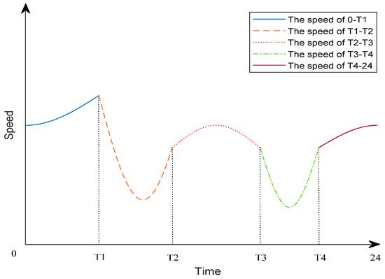
Figure 1.
Variation trend of vehicle speed.
Figure 1 is taken as an example to illustrate the driving time of the vehicle from node to node . If the time when vehicle leaves node belongs to , there are two situations of when vehicle arrives at node from node : (1) , the time that vehicle arrives at node from node belongs to , so the time that vehicle traveled from node to node can be calculated according to and in . (2) , the time that vehicle arrives at node from node does not belong to , so vehicle maybe cross period to arrive at node . represent the distances that vehicle traveled in each time period. The total travel time can be described as . represents the travel time that vehicle traveled in time period, which can be obtained according to the and in .
2.4. Mathematical Model
The objective is to minimize the total distribution cost, including fixed cost, fuel consumption cost and time window penalty cost.
The MDJDVRP-TDN model is as follows:
Constraint (5) indicates that vehicles sent from the depot cannot exceed the maximum vehicle number limit. Constraint (6) represents the constraint of vehicle entry and exit balance. Constraint (7) represents that each customer is only served by the vehicle once, and the demand is not allowed to split. Constraint (8) represents the relationship between two variables. Constraint (9) calculates the vehicle load. Constraint (10) represents the constraint on vehicle payload capacity. Constraint (11) calculates the time that vehicle leaves customer . In constraint (12), the time that vehicle arrives at the node can be obtained by calculating the upper limit of the integral according to the speed function. Constraint (13) indicates that the vehicle can only set out after the depot has worked. Constraint (14) indicates that vehicle must return to the depot before the depot has finished work. Constraint (15) is to eliminate the sub-loop. Constraints (16) and (17) define the attributes of decision variables.
3. Heuristic
The vehicle routing problem is a classic NP-hard problem, and the heuristic algorithm derived in recent years can find a satisfactory solution within a reasonable time range, which is an effective method for solving vehicle routing problems [23,24]. Genetic algorithm has the advantages of simple operation and easy to combine with other algorithms. The variable neighborhood search algorithm has a strong search ability. In this paper, HGAVNS is designed by combining the advantages of variable neighborhood search algorithms and genetic algorithms.
3.1. Coding and Decoding and Generation of Initial Population
In this paper, two methods are used to generate the initial population by integer coding. The first method is to use the nearest neighbor insertion method to generate a customer array. The nearest neighborhood insertion method can help the algorithm to obtain a better solution and accelerate the convergence speed. It selects the customer with the smallest and the shortest distance from the depot as the first customer, and then through the nearest neighbor insertion method to add other customers to the customer array. The second method is to use the Logistics mapping equation to generate the initial population. Logistic mapping equation can increase the randomness and diversity of the initial solution by utilizing the inherent randomness of a chaotic system. The logistic mapping equation is shown in Equation (18):
represents the state of population in period, . is a control parameter, .
Each chromosome in the population is tested for payload constraint. If the vehicle does not meet the payload constraint and cannot continue to serve subsequent customers, it will return to the depot and another vehicle will be sent from the depot to continue to serve other customers.
Figure 2 is taken as an example to illustrate the decoding of a chromosome. The customer arrangement (chromosome) has been generated as , and the first vehicle is sent from the depot to provide service. When the vehicle reaches customer 1, it cannot serve subsequent customers due to the payload constraint. The second vehicle is sent to serve subsequent customers and so on until the last customer has been served. The starting and ending depots are determined for each route, and depots are represented by numbers 8 and 9. The starting and ending depots for vehicle 1 are 8 and 9, and the starting and ending depots for vehicle 2 are both 9.
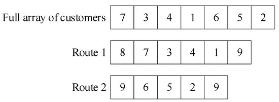
Figure 2.
Schematic diagram of decoding.
3.2. Fitness Function
In this paper, the minimum value problem is solved. The fitness function value of chromosomes is the reciprocal of the objective function value, so the smaller the objective function value is, the larger the fitness value is, the better the chromosome is, and the greater the probability of entering the next generation is. The fitness function of chromosome is shown in Equation (19).
is the objective function value of chromosome .
3.3. Selection Operation
This paper adopts the combination of elite and roulette selection strategies. Such a selection strategy ensures that the best chromosomes from each generation are retained to the next generation, but also increases the diversity of solutions to avoid the algorithm falling into local optimum. The basic idea of the elite retention strategy is to retain the optimal individual in each iteration and replace the individual with the smallest fitness function value in the contemporary population. The roulette selection strategy is to calculate the probability that each chromosome in the population will be inherited to the next generation, and its probability is proportional to the fitness function value of the chromosome. The higher the fitness function value of the chromosome, the greater the probability that the chromosome will be selected into the next generation cycle. The selection process is repeated until a population of the same size as the parent is formed. The combination of the two selection strategies ensures both the diversity and the quality of solutions and improves the convergence speed of the algorithm.
3.4. Variable Neighborhood Search
Variable neighborhood search strategy has strong search ability. Crossover and mutation operations in traditional genetic algorithms are replaced by variable neighborhood search strategy, which can increase the performance of the algorithm. Variable neighborhood search strategy: neighborhood structure , the first neighborhood structure starts to search to chromosomes . If the improved solution is not found within the search times, the next neighborhood structure will continue to search; Otherwise, , and the first neighborhood structure is searched again. In this paper, five neighborhood structures are adopted, namely, insertion, swap, 2-insertion, 2-opt and or-opt.
3.4.1. Neighborhood Structure
(1) Insertion. Node and node are selected randomly, and then node is inserted after node . As shown in Figure 3a, node 1 and node 5 are selected randomly, and node 1 is inserted after node 5.
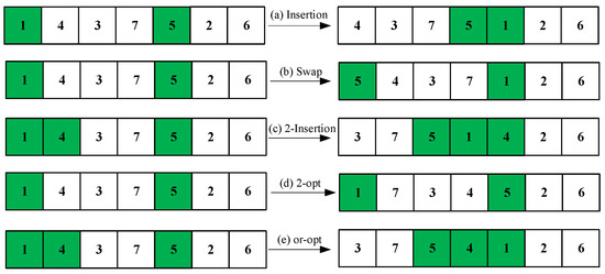
Figure 3.
Schematic diagram of the variable neighborhood search strategy.
(2) Swap. Node and node are selected randomly, and then the positions of node and node are swapped. As shown in Figure 3b, node 1 and node 5 are selected randomly, and the positions of node 1 node 5 are swapped.
(3) 2-Insertion. Continuous node , and discontinuous node are selected randomly, and node and node are inserted after node . As shown in Figure 3c node 1 and node 4 are selected randomly, and then node 1 and node 4 are inserted after node 5.
(4) 2-opt. Node and node are selected randomly, and then reverse the order of other nodes between node and node . As shown in Figure 3d, node 1 and node 5 are selected randomly, and the position of node 1 and node 5 are kept and reverse the position of other nodes between node 1 and node 5.
(5) or-opt. Consecutive node and node are selected randomly, and then insert them in reverse order after node . As shown in Figure 3e, node 1 and node 4 are selected randomly, and then insert them in reverse order after node 5.
3.4.2. Adaptive Mechanism
In this paper, we designed adaptive neighborhood search times to balance the breadth and depth required by evolution. The adaptive neighborhood search times strategy is shown as Equation (20).
are search times and adaptive search times, respectively. is the maximum iteration times, and is the current iteration times. represents round down. It can be seen from Equation (20), at the beginning of iteration that the population has a low number of search times . With the increase of iteration times, the search times of population search strategy gradually increase. Based on maintaining population diversification, the exploration of population depth should be increased.
4. Experimental Analysis
At present, there are no standard instances of MDJDVRP-TDN. In this paper, the standard instances of multi-depot vehicle routing problem (MDVRP) and time dependent vehicle routing problem with time window (TDVRPTW) are selected to verify the algorithm, and then the MDJDVRP-TDN instances are designed to conduct experiments on the problems. Finally, the sensitivity analysis of vehicle speed and the impact of vehicle load on fuel consumption are conducted.
MATLAB R2018b is used for algorithm programming. The computer operating system is Window10, the operating memory is 8G, the CPU is Intel(R)Core(TM) I7-7700, and the main frequency is 3.60 GHz. After repeated testing, the algorithm parameters are set as follows: population size , maximum number of iterations , adaptive parameter , . Parameter settings are related to the scale of instances. When , we set , and . When , we set , and . When , we set , and .
4.1. MDVRP Standard Instances Verification
To test the performance of the algorithm proposed, the MDVRP instances are downloaded from the standard instances library (source: https://neo.lcc.uma.es/vrp/vrp-instances/multiple-depot-vrp-instances/ (accessed on 1 September 2021)). Table 1 shows the solution results of genetic algorithm (GA) [25], iterative local search (ILS) [26], adaptive memetic algorithm and variable neighborhood search (AMAVNS) [27], and HGAVNS to MDVRP standard instances of different scales. Where represents the customer scale, represents the known optimal solution, is the optimal solution obtained by each algorithm, %Dev represents the deviation between the optimal solution obtained by each algorithm and the known optimal solution. The numbers in bold are the algorithm that finds the best-known solution. Figure 4 shows the optimal routes schematic diagram of some instances.

Table 1.
Comparison results of MDVRP standard instances.
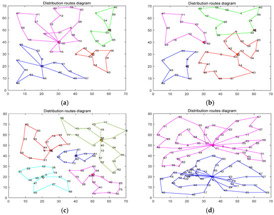
Figure 4.
Optimal routes diagram of some standard instances. (a) Optimal routes of instance p01; (b) Optimal routes of instance p02; (c) Optimal routes of instance p03; (d) Optimal routes of instance p04.
As can be seen from Table 1, GA does not work out the optimal solution of the instances, and the maximum deviation from the known optimal solution is 9.05% and the minimum deviation is 0.73%. ILS has not worked out the optimal solution of the instances, and the maximum deviation from the known optimal solution is 6.15% and the minimum deviation is 2.55%. AMAVNS works out the optimal solution of 2 instances. In other instances, it does not work out the optimal solution, and the maximum deviation from the known optimal solution is 3.86% and the minimum deviation is 0.80%. In this paper, HGAVNS works out the optimal solutions of 4 instances. In other instances, the maximum deviation from the known optimal solution is 1.72% and the minimum deviation is 0.01%. The solution results of HGAVNS are better than those of the other four algorithms, and the deviation from the optimal solution is less than 2%. It can be seen from the analysis results in Table 1 that the HGAVNS has a good solving performance and can effectively solve small-, medium- and large-scale instances. This is mainly because HGAVNS uses the logistic mapping equation to generate the initial population, which increases the diversity and randomness of the population. The adaptive mechanism designed during algorithm iteration balances the depth and breadth of population evolution and improves the solving performance of the algorithm. So, it can get a better solution in a reasonable time range.
4.2. TDVRPTW Standard Instances Verification
In this section, TDVRPTW standard instances are used to verify the algorithm and compared with iterative route construction and improvement (IRCI) [28] and parallel-simulated annealing (p-SA) [29]. Table 2 shows the solution results of TDVRPTW standard instances solved by IRCI, p-SA and HGAVNS. Where is the number of vehicles required, and represents the optimal solution obtained by each algorithm.
Table 2.
Comparison of TDVRPTW standard instances.
It can be seen from Table 2 that the optimal solutions of the four groups of time-dependent functions use 10 vehicles, and the solution results are stable. Compared with IRCI, the optimal solutions obtained by HGAVNS are superior to IRCI. Compared with p-SA, only the optimal solutions obtained by instances TD3a and TD3c are relatively poor, and the other 10 instances are superior to p-SA. As can be seen from the analysis results in Table 2, compared with IRCI and p-SA, HGAVNS has stable solution performance and can get better results. This is mainly because HGAVNS uses two methods to generate the initial population, which increases the diversity and randomness of the population. The five neighborhood structures increase the depth search ability of the algorithm. So, it can get a better solution in a reasonable time range.
4.3. MDJDVRP-TDN Instances Verification
Since there are no MDJDVRP-TDN standard instances in existing research, this paper modifies the MDVRP standard instance of p04 (source: https://neo.lcc.uma.es/vrp/vrp-instances/multiple-depot-vrp-instances/ (accessed on 1 September 2021)) to generate MDJDVRP-TDN instances, which involves 100 customers and 4 depots. The work time window of depots are , the waiting cost per unit time is 20 and the delay cost per unit time is 30. Unit cargo handling time is 10. The cost parameters of delivery vehicles are shown in Table 3.
Table 3.
Cost parameters.
Roads in the distribution area road network are divided into three types, namely trunk road, secondary trunk road and branch road, as shown in Figure 5, which the red line represents trunk road, the black line represents secondary trunk road, and nodes not connected by lines are in the branch road. The yellow stars in Figure 5 represent depots. Figure 6 shows the speed changes of different types of roads. The red line represents the vehicle speed of trunk roads, the black line represents the vehicle speed of secondary trunk roads, and the blue line represents the vehicle speed of branch roads. Table 4 shows the results of HGAVNS for MDJDVRP-TDN instances for 10 times, which represents the total distribution cost, represents the best solution, represents the average solution, represents the worst solution, CPU represents the running time, %Dev represents the deviation between the solution of each time and the best solution. The optimal distribution scheme is given in Table 5, which is the distribution route of each vehicle.
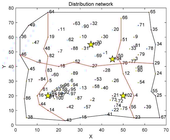
Figure 5.
Distribution network.
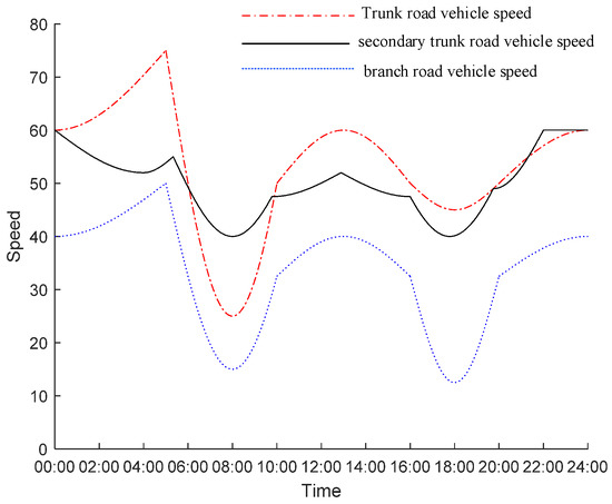
Figure 6.
Variation trend of vehicle speed.
Table 4.
Results of ten times.
Table 5.
Optimal distribution scheme.
It can be seen from Table 4 that the deviates from the best solution within 5%, and we get the best solution two out of ten times, so the solution is relatively stable. In the iterative process, the algorithm can converge to the optimal within 200s, and the algorithm has high solving efficiency.
It can be seen from Table 5 that 16 vehicles are needed to serve these 100 customers, in which the total distribution cost is 5749.06. No. 1, 2, 5, 6, 8, 9, 10, 12 and 14 vehicles return to the original depot, and the remaining 7 vehicles do not return to the original depot and return to the depot closest to the last customer visited by the vehicle, which can reduce the travel distance, and avoid roundabout transportation, and thus reduce the total distribution cost.
To verify the performance of the HGAVNS for solving different scales instances, MDJDVRP-TDN instances with customer scales of 50, 75 and 100 are randomly generated. Each instance is solved 10 times. Table 5 records the optimal solution among the 10 solutions, where is the number of depots and is the number of vehicles used in the distribution scheme.
As can be seen from Table 6, for instances with the same customer scale, geographic coordinates and customer demand have an important influence on the formulation of the scheme. For the instances with the same customer scale, the difference of total distribution cost is at least 10.43 and at most 569.31.
Table 6.
Solution results of different scales instances.
4.4. Sensitivity Analysis
4.4.1. Vehicle Speed Analysis
This section analyzes the impact of different vehicle speeds on the distribution scheme, and sets 5 different vehicle speeds, and makes a comparative analysis of the optimal distribution scheme under different vehicle speeds. Where Case1 is the vehicle speed set in Section 4.3; Case2 and Case3 are increased and decreased by 6 km/h respectively based on the vehicle speed set in Section 4.3. In Case4, it is assumed that the vehicle speed of the trunk road and the secondary road is constant 55 km/h and 45 km/h, while the vehicle speed of the branch road is constant. In Case5, it is assumed that the vehicle speed of the trunk road and the secondary road is constant 50 km/h, and the vehicle speed of the branch road is constant. Table 7 shows the optimal solution under different vehicle speeds, and the last column is the deviations of optimal solution between Case2-Case5 and Case1, in which is the sum of penalty costs of each vehicle’s time window, is the sum of fuel consumption costs of each vehicle.
Table 7.
Vehicle speed sensitivity analysis results.
It can be seen from Table 7 that the change of vehicle speed will lead to the change of time window penalty cost and fuel consumption cost. As can be seen from the second column in Table 7, the time window penalty cost in Case2 is the lowest, mainly because the assumed vehicle speed increases by 6 km/h. The time window penalty cost in Case3 is the highest, mainly because the assumed vehicle speed decreases by 6 km/h. It can be seen from the third column that the fuel consumption cost is the lowest in Case2 and the highest in Case4. As can be seen from the fourth column, the number of vehicles in use under 5 different vehicle speeds is equal. As can be seen from the last column, only when the vehicle speed increases by 6 km/h, the total distribution cost decreases by 1.77%, and in other cases, the total distribution cost increases by 7.78% at most and 2.48% at least. Through the analysis of the above results, the time window penalty cost, fuel consumption cost and total distribution cost of the optimal distribution scheme are greatly different when the vehicle speed is different, and the vehicle speed has a great influence on the formulation of the distribution scheme. In this paper, the multi-depot joint distribution vehicle routing problem considering energy consumption under time-dependent networks is closer to the actual transportation situation of logistics enterprises and has important research significance.
4.4.2. Influence Analysis of Load on Fuel Consumption
In the above experiments, there is a linear relationship between vehicle fuel consumption and vehicle load. In this section, the influence of load on fuel consumption is analyzed. It is assumed that the fuel consumption per unit distance of the distribution vehicle is fixed, and the final fuel consumption is only related to the travel distance, not the vehicle load. According to Equation (1) and parameter settings in Section 4.3, it can be known that the fuel consumption per unit distance of unit cargo is . We set the fuel consumptions per unit distance are , and respectively. Table 8 shows the solution results of different unit distance fuel consumption, where , , and respectively represent the distribution cost under the consideration of the influence of load on fuel consumption and different parameter values of the fuel consumptions per unit distance. %Dev1, %Dev2 and %Dev3 are the deviations between the total distribution cost calculated by using fixed fuel consumption per unit distance and the total distribution cost calculated by considering the impact of load on fuel consumption.
Table 8.
Influence analysis of load on fuel consumption.
As can be seen from Table 8, the maximum deviation of the total distribution cost calculated by using fixed fuel consumption per unit distance is −24.98% and the minimum deviation is 0.87% compared with the total distribution cost calculated by considering the impact of load on fuel consumption. The experimental results show that the total distribution cost is closer to reality considering the influence of load on energy consumption.
5. Conclusions
This paper studies the multi-depot joint distribution vehicle routing problem considering energy consumption with time-dependent networks and draws the following conclusions:
- (1)
- This paper establishes the MDJDVRP-TDN model based on fixed cost, fuel consumption cost and time window penalty cost, which truly reflects the cost composition of logistics enterprises’ distribution vehicles and provides the theoretical basis for logistics enterprises to formulate vehicle scheduling schemes.
- (2)
- The MDJDVRP-TDN model can truly reflect the continuous variation trend of vehicle speed, and the division of road types in the regional road network is the deepening and expansion of the vehicle routing problem.
- (3)
- Using the nearest neighbor insertion method and Logistic mapping equation to generate the initial population, which not only ensures the quality of the initial solution but also improves the randomness of the initial solution. The selection operation combining elite reservation and roulette improves the diversity of the population and the convergence speed of the algorithm. Five kinds of variable neighborhood search structures are designed to improve the local search capability and improve the performance of the algorithm. Adaptive neighborhood search times strategy is used to balance the diversification and depth search of population.
This study can provide a solution for transportation enterprises with multiple depots to develop a multi-depot joint distribution scheme according to the changes in historical road networks. However, vehicle scheduling will be affected by real-time changes of road networks, especially by some emergencies. Therefore, how to plan vehicle routes according to real-time traffic information is a direction that needs further research in the future.
Author Contributions
D.H. and H.F. provided the core idea of this paper, analyzed the data, and wrote the manuscript. X.R. contributed to the conceptualization of this paper, data collection, and provision of valuable comments. All authors have read and agreed to the published version of the manuscript.
Funding
This work was supported by the Special Project of National Emergency Management System Construction of the National Social Science Fund of China, Grant number 20VYJ024.
Institutional Review Board Statement
Not applicable.
Informed Consent Statement
Not applicable.
Data Availability Statement
Not applicable.
Conflicts of Interest
The authors declare no conflict of interest.
References
- Xu, Z.; Elomri, A.; Pokharel, S.; Mutlu, F. A model for capacitated green vehicle routing problem with the time varying vehicle speed and soft time windows. Comput. Ind. Eng. 2019, 137, 106011. [Google Scholar] [CrossRef]
- Fan, H.; Yang, X.; Li, D.; Li, Y.; Liu, P. Half-open multi depot vehicle routing problem based on joint distribution mode of fresh food. Comput. Integ. Manufact. Syst. 2019, 25, 256–266. [Google Scholar]
- Bao, C.; Zhang, S. Route optimization of cold logistics in joint distribution: With consideration of carbon emission. Ind. Eng. Manag. 2018, 23, 95–100, 107. [Google Scholar]
- Yuan, S.; Meng, C.; Ting, Q.; Wei, L. Vehicle routing problem of an innovative B2C and O2O joint distribution service. Procedia CIRP 2019, 83, 680–683. [Google Scholar]
- Yang, X.; Fan, H.; Zhang, X.; Li, Y. Optimization of multi-depot open vehicle routing problem with fuzzy window. Comput. Integ. Manufact. Sys. 2016, 22, 1768–1778. [Google Scholar]
- Alinaghian, M.; Shokouhi, N. Multi-depot multi-compartment vehicle routing problem, solved by a hybrid adaptive large neighborhood search. Omega 2018, 76, 85–99. [Google Scholar] [CrossRef]
- Ge, X.; Zhou, D. Vehicle routing problem of multi-distribution centers with cross-docking in the supply chain. Control Decis. 2018, 33, 2169–2176. [Google Scholar]
- Wang, Y.; Assogba, K.; Fan, J.; Liu, Y. Multi-depot green vehicle routing problem with shared transportation resource: Integration of time-dependent speed and piecewise penalty cost. J. Clean. Prod. 2019, 232, 12–29. [Google Scholar] [CrossRef]
- Li, Y.; Soleimani, H.; Zohal, M. An improved ant colony optimization algorithm for the multi-depot green vehicle routing problem with multiple objectives. J. Clean. Prod. 2019, 227, 1161–1172. [Google Scholar] [CrossRef]
- Sabar, N.R.; Bnaskar, A.; Turky, A.; Song, A. A self-adaptive evolutionary algorithm for dynamic vehicle routing problems with traffic congestion. Swarm Evol. Comput. 2018, 44, 1018–1027. [Google Scholar] [CrossRef]
- Zhang, C.; Zhang, Y. Study on vehicle route Problem under dynamic road system. J. Transp. Eng. Inf. 2017, 15, 112–118. [Google Scholar]
- Haghani, A.; Jung, S. A dynamic vehicle routing problem with time-dependent travel times. Comput. Oper. Res. 2005, 32, 2959–2986. [Google Scholar] [CrossRef]
- Cai, Y.; Tang, Y.; Cal, H. Adaptive ant colony optimization for vehicle routing problem in time varying networks environment. Appl. Res. Comput. 2015, 32, 2309–2312, 2346. [Google Scholar]
- Wu, Y.; Ma, A. Time-dependent production-delivery problem with time windows for perishable foods. Syst. Eng. Theory Pract. 2017, 37, 172–181. [Google Scholar]
- Liu, C.; Kou, G.; Zhou, X.; Peng, Y.; Sheng, H. Time-dependent vehicle routing problem with time windows of city logistics with a congestion avoidance approach. Knowl. Based Syst. 2020, 188, 104813. [Google Scholar] [CrossRef]
- Donati, A.V.; Montemanni, R.; Casagrande, N.; Rizzoli, A.E.; Gambardella, L.M. Time dependent vehicle routing problem with a multi ant colony system. Eur. J. Oper. Res. 2008, 185, 1174–1191. [Google Scholar] [CrossRef]
- Duan, Z.Y.; Lei, Z.X.; Sun, S.; Yang, D.Y. Multi-objective robust optimization method for stochastic time-dependent vehicle routing problem. J. Southwest Jiaotong Univ. 2019, 54, 565–572. [Google Scholar]
- Deng, Y.; Zhu, W.; Li, H.; Zheng, Y. Multi-type ant system algorithm for the time dependent vehicle routing problem with time windows. IEEE Access 2018, 29, 625–638. [Google Scholar]
- Zhang, C.; Zhao, Y.; Leng, L. A Hyper-Heuristic Algorithm for Time-Dependent Green Location Routing Problem with Time Windows. IEEE Access 2020, 8, 83092–83104. [Google Scholar] [CrossRef]
- Zhang, K.; Ji, Q. Research on multi-depot half-open vehicle routing problem with time-varying speed. J. Syst. Simul. 2021, 1–11. [Google Scholar] [CrossRef]
- Xiao, Y.; Zhao, Q.; Kaku, I.; Xu, Y. Development of a fuel consumption optimization model for the capacitated vehicle routing problem. Comput. Oper. Res. 2012, 39, 1419–1431. [Google Scholar] [CrossRef]
- Yang, H. Research of Urban Recurrent Congestion Evolution Based on Taxi GPS Data; Harbin Institute of Technology: Harbin, China, 2018. [Google Scholar]
- Fava, L.P.; Furtado, J.C.; Helfer, G.A.; Barbosa, J.L.V.; Beko, M.; Correia, S.D.; Leithardt, V.R.Q. A Multi-Start Algorithm for Solving the Capacitated Vehicle Routing Problem with Two-Dimensional Loading Constraints. Symmetry 2021, 13, 1697. [Google Scholar] [CrossRef]
- Nasri, M.; Hafidi, I.; Metrane, A. Multithreading Parallel Robust Approach for the VRPTW with Uncertain Service and Travel Times. Symmetry 2020, 13, 36. [Google Scholar] [CrossRef]
- Karakatic, S.; Podgorelec, V. A survey of genetic algorithms for solving multi depot vehicle routing problem. Appl. Soft Comput. J. 2015, 27, 519–532. [Google Scholar] [CrossRef]
- Tlili, T.; Krichen, S.; Drira, G.; Faiz, S. On solving the multi-depot vehicle routing problem. In Proceedings of the 3rd International Conference on Advanced Computing, Networking and Informatics, Orissa, India, 23–25 June 2015; pp. 103–108. [Google Scholar]
- Fan, H.; Liu, P.; Hou, D. The multi-depot vehicle routing problem with simultaneous deterministic delivery and stochastic pickup based on joint distribution. Acta Auto Sin. 2021, 47, 1–5. [Google Scholar]
- Figliozzi, M. The time dependent vehicle routing problem with time windows: Benchmark problems, an efficient solution algorithm, and solution characteristics. Transp. Res. Part E Logist. Transp. Rev. 2012, 48, 616–636. [Google Scholar] [CrossRef]
- Mu, D.; Wang, C.; Wang, S.; Zhou, S. Solving TDVRP based on parallel-simulated annealing algorithm. Comput. Integr. Manuf. Syst. 2015, 21, 1626–1636. [Google Scholar]
Publisher’s Note: MDPI stays neutral with regard to jurisdictional claims in published maps and institutional affiliations. |
© 2021 by the authors. Licensee MDPI, Basel, Switzerland. This article is an open access article distributed under the terms and conditions of the Creative Commons Attribution (CC BY) license (https://creativecommons.org/licenses/by/4.0/).