On Unconditionally Stable New Modified Fractional Group Iterative Scheme for the Solution of 2D Time-Fractional Telegraph Model

Abstract

In this study, a new modified group iterative scheme for solving the two-dimensional (2D) fractional hyperbolic telegraph differential equation with Dirichlet boundary conditions is obtained from the 2h-spaced standard and rotated Crank–Nicolson FD approximations. The findings of new four-point modified explicit group relaxation method demonstrates the rapid rate of convergence of proposed method as compared to the existing schemes. Numerical tests are performed to test the capability of the group iterative scheme in comparison with the point iterative scheme counterparts. The stability of the derived modified group method is proven by the matrix norm algorithm. The obtained results are tabulated and concluded that exact solutions are exactly symmetric with approximate solutions.

1. Introduction

Partial differential equations have a wide range of applications in applied sciences, including wave propagation, electric signal propagation, and atomic physics [1,2,3,4,5]. In recent years, several numerical techniques for multidimensional hyperbolic partial differential equations have been developed [6,7,8,9,10,11]. For example, Gao and Chi [12] solved one-space-dimensional linear hyperbolic model based on unconditionally stable difference schemes. Youssef [13] studied the class of fractional functional integro-differential equations of the Caputo–Katugampola type. Many techniques have been used to solve fractional partial differential equations using the Caputo and the Caputo–Fabrizio type operators [14,15,16]. Lai and Liu [17] solved the second order fractional partial differential equation using the Galerkin finite element method and Riesz fractional derivative. Akram et al. [18,19] proposed unconditionally stable methods for the fractional hyperbolic models via B-spline approaches. Several years before this, the unconditionally stable alternating dimension implicit schemes for 2D and three-dimensional hyperbolic equations were derived by Mohanty and Jain [20,21]. Later, Mohanty [22] also proposed new difference approach for the solution of telegraphic equation. Meanwhile, Dehghan and Mehebbi [23,24] suggested numerical approaches for 2D linear hyperbolic equations by applying collocation finite difference (FD) approximations. The other derived numerical schemes for hyperbolic partial differential equations can be seen in [25,26].

Most of the researchers discretized their presented issues using various types of discretization techniques such as the FD approach [27], the finite element scheme [28], and the boundary element approach [29], among others. A sparse system of linear equations is obtained in the following form:

$$\mathbf{A}\upsilon =\mathbf{b}.$$

(1)

Iterative approaches are ideal for solving this sparse system of linear equations in this case. These iterative methods utilized all of the grid points in the solution domain ${\mathrm{\Omega }}_{\mathit{h}}$, ($\mathit{h}$ is grid spacing in both x and y direction) including the boundary points to achieve the convergence. Due to the involvement of all the grid knots in the suggested domain ${\mathrm{\Omega }}_{\mathit{h}}$, these methods are forced to utilize a lot of algebraic operations in the iterative loop that resulted in large computational complexities and consume more execution time per iteration for their evaluation.

A number of studies on iterative schemes have been presented to improve the convergence rate in solving Equation (1). One of them is the establishment of the group iterative algorithms capable of reducing iterative process convergence times. We divide the entire domain into groups of knots, and values on each group are explicitly assessed using properly stated FD formulas that reduce the overall amount of arithmetic operations. Evans [30] used the Explicit Group (EG) iterative method to solve the Poisson problem by creating a 4-point block iterative scheme. Evans and Yousif [31,32], Evans and Sahimi [33], Evans and Hasan [11] and Kew and Ali [10] have extensively researched a range of EG iterative techniques for various forms of partial differential equations based on this idea. In addition, another type of group iterative method based on the half-sweep technique called Explicit Decoupled Group (EDG) approach is presented by Abdullah [34] for solving Poisson differential equation. Later, Yousif and Evans [35] and Ibrahim and Abdullah [36] initiated half-sweep approach via EDG iterative scheme for the numerical solution of the elliptic partial differential and diffusion equations, respectively. Later, many authors utilized this approach for several other types of differential equations.

The use of modified groups quarter-sweep technique have been widely shown to provide faster rate of convergence. This approach can be constructed by implementation of FD approximation with 2h grid spacing in the discretized region. The quarter-sweep approach’s basic concept is based on time reduction techniques that use nearly the quarter grid points of the solution region and these points are treat as iterative points that involved in the iterative process. Just by using the quarter grid points of the suggested domain, iterative process reduces the computational complexity of the algorithm and hence ultimately decreases the execution of time per iteration. The remaining grid points that are not included in the iterative process are referred to as direct points, and they can be evaluated directly using the point iterative approach. On the basis of this concept, Othman and Abdullah [37] discovered Modified Explicit Group (MEG) iterative approach for the numerical solution of 2D Poisson differential equation by utilizing the quarter grids stencil of the solution domain and results were found much better and faster than the results obtained from EDG iterative method derived from utilizing the half grids stencil for the same 2D Poission equation [34].

Many authors applied this technique on several types of partial differential equations with promising results [9,38]. Because of the technique’s success with integer derivative PDEs, researchers are now attempting to adapt it to fractional differential equations. Balasim and Ali [39,40,41] recently published preliminary work on parabolic partial differential equations of fractional order. The main purpose of this research is to investigate the capability of this technique for solving the 2D fractional telegraph equation on a family of four points with 2h grid spacing.

Consider the second-order time-fractional hyperbolic telegraph equation [6],

$$\frac{{\partial }^{2\alpha }\mathrm{{\rm Y}}}{\partial t^{2\alpha }}+2\mu (x,y,t)\frac{{\partial }^{\alpha }\mathrm{{\rm Y}}}{\partial t^{\alpha }}+{\eta }^2(x,y,t)\mathrm{{\rm Y}}=a(x,y,t)\frac{{\partial }^2\mathrm{{\rm Y}}}{\partial x^2}+b(x,y,t)\frac{{\partial }^2\mathrm{{\rm Y}}}{\partial y^2}+f(x,y,t),$$

(2)

where $1/2<\alpha <1$, $\mu (x,y,t)>0,\eta (x,y,t)>0.\mathrm{Also},a(x,y,t)>0,$$b(x,y,t)$ are positive real constants and $f(x,y,t)$ is the forcing term. If $\eta (x,y,t)=0,$ then Equation (2), reduces to the fractional damped wave equation.

Initial and boundary conditions are as follows:

$$\mathrm{{\rm Y}}(x,y,0)={\psi }_1(x,y),{\mathrm{{\rm Y}}}_t(x,y,0)={\psi }_2(x,y),$$

$$\mathrm{{\rm Y}}(0,y,t)=g_1(y,t),\mathrm{{\rm Y}}(L,y,t)=g_2(y,t),$$

$$\mathrm{{\rm Y}}(x,0,t)=g_3(x,t),\mathrm{{\rm Y}}(x,L,t)=g_4(x,t),$$

where ${\mathrm{\Omega }}_{\Delta }=\{(x,y,t)/0<x,y<L,0\le t\le T\}.$

Discretize the spatial domain as $t_k=k\tau ,k=0,1,2,\cdots N$, $x_i=i\Delta x,i=0,1,2,\cdots M_x$ and $y_i=j\Delta y,j=0,1,2,\cdots M_y$ where $\tau =\frac{T}{N}$, $\Delta x=\frac{L}{M_x}$ and $\Delta y=\frac{L}{M_y}$ and N, $M_x$ and $M_y$ are the positive integers. The grid points of the discretized solution domain are given by $(x_i,y_j,t_k)=(i\Delta x,j\Delta y,k\tau )$. The exact solution of the fractional differential Equation (2) is ${\mathrm{{\rm Y}}}_{i,j,k}$, while the approximate solution is ${\upsilon }_{i,j,k}$ and consider the following,

$$f(x_i,y_j,t_k)=f_{i,j}^k,\hspace{1em}a(x_i,y_j,t_k)=a_{i,j}^k,\hspace{1em}b(x_i,y_j,t_k)=b_{i,j}^k,$$

$$\eta (x_i,y_j,t_k)={\eta }_{i,j}^k,\hspace{1em}\mu (x_i,y_j,t_k)={\mu }_{i,j}^k.$$

The Caputo’s time fractional derivative is defined as follows:

$$\frac{{\partial }^{\alpha }\upsilon (x,y,t)}{\partial t^{\alpha }}=\frac{1}{\mathrm{\Gamma }(m-\alpha )}{\int }_0^t\frac{\partial {\upsilon }^m(x,y,\xi )}{\partial {\xi }^m}\frac{d\xi }{{(t-\xi )}^{\alpha +1-m}},m-1<\alpha <m.$$

(3)

The following two equations of Caputo’s fractional derivatives of order $2\alpha$ and $\alpha$ can be derived from Equation (3) by using the first and second time differential operators.

$$\frac{{\partial }^{2\alpha }\upsilon (x_i,y_j,t_{k+1/2})}{\partial t^{2\alpha }}=\frac{1}{\mathrm{\Gamma }(3-2\alpha ){\tau }^{2\alpha }}\sum _{s=1}^k{\omega }_s^{*}[{\upsilon }_{i,j}^{k-s+2}-2{\upsilon }_{i,j}^{k-s+1}+{\upsilon }_{i,j}^{k-s}]+O\left({\tau }^{3-2\alpha }\right)$$

(4)

where ${\omega }_s^{*}=s^{2(1-\alpha )}-{(s-1)}^{2(1-\alpha )},s=1,2\cdots k$ and

$$\frac{{\partial }^{\alpha }\upsilon (x_i,y_j,t_{k+1/2})}{\partial t^{\alpha }}=\frac{1}{\mathrm{\Gamma }(2-\alpha ){\tau }^{\alpha }}\sum _{s=1}^k{\omega }_s[{\upsilon }_{i,j}^{k-s+2}-{\upsilon }_{i,j}^{k-s+1}]+O\left({\tau }^{2-\alpha }\right)$$

(5)

where ${\omega }_s=s^{1-\alpha }-{(s-1)}^{1-\alpha },s=1,2\cdots k.$

The structure of this paper is as follows: The derivation of MFEG iterative scheme based on 2h-spaced standard Crank–Nicolson FD approximation is explained in Section 2. Section 3 discusses the MFEG iterative scheme’s stability and convergence. Numerical Experimental and Results are discussed in Section 4. The Conclusions are provided in the last Section 5.

2. Modified Fractional Explicit Group (MFEG) Iterative Scheme

The $\mathit{h}$-spaced point and group iterative schemes for 2D fractional telegraph equation have been derived by Ali and Ali in [6]. The following standard 2h-spaced iterative scheme can be obtain by utilizing standard 2h-spaced Crank–Nicolson scheme for space-derivatives and Caputo fractional derivatives from Equations (4) and (5) for time-derivatives in Equation (2), we have the following expression,

$${\upsilon }_{i,j}^{k+1}=\frac{1}{(p_1+p_2+r_1/4+r_2/4+q)}[\frac{r_1}{8}({\upsilon }_{i-2,j}^{k+1}+{\upsilon }_{i+2,j}^{k+1})+\frac{r_2}{8}({\upsilon }_{i,j-2}^{k+1}+{\upsilon }_{i,j+2}^{k+1})$$

$$+\frac{r_1}{8}({\upsilon }_{i-2,j}^k+{\upsilon }_{i+2,j}^k)+\frac{r_2}{8}({\upsilon }_{i,j-2}^k+{\upsilon }_{i,j+2}^k)+(p_1(1-{\omega }_2)-p_2+q(2-{\omega }_2^{*})-r_1/4-r_2/4){\upsilon }_{i,j}^k$$

$$+(p_1{\omega }_k+2q{\omega }_k^{*}){\upsilon }_{i,j}^1-q{\upsilon }_{i,j}^{k-1}+p_1\sum _{s=2}^{k-1}({\omega }_s-{\omega }_{s-1}){\upsilon }_{i,j}^{k-s+1}+q\sum _{s=2}^{k-1}(2{\omega }_s^{*}-{\omega }_{s-1}^{*}){\upsilon }_{i,j}^{k-s+1}$$

$$-q\sum _{s=2}^{k-1}{\omega }_s^{*}{\upsilon }_{i,j}^{k-s}+m_0{f}_{i,j}^{k+1/2}]$$

(6)

with initial and boundary conditions,

$${\upsilon }_{i,j}^0={\psi }_1(x_i,y_j),\upsilon t_{i,j}^0={\psi }_2(x_i,y_j)$$

$${\upsilon }_{0,j}^k=g_1(y_j,t),{\upsilon }_{L,j}^k=g_2(y_j,t)$$

$${\upsilon }_{i,0}^k=g_3(x_i,t),{\upsilon }_{i,L}^k=g_4(x_i,t)$$

for all $i=2,4\cdots M_x-2$, $j=2,4\cdots M_y-2$ and $k=0,1,2,3\cdots N$ where,

$$m_0={\tau }^{2\alpha }\mathrm{\Gamma }(3-2\alpha )\mathrm{\Gamma }(2-\alpha ),q=\mathrm{\Gamma }(2-\alpha )$$

$$p_1=2{\tau }^{\alpha }\mathrm{\Gamma }(3-2\alpha ){\mu }_{i,j}^k,p_2=m_0{2}^{-1}{\left({\eta }_{i,j}^k\right)}^2$$

$$r_1=a_{i,j}^k\frac{m_0}{{(\Delta x)}^2},r_2=b_{i,j}^k\frac{m_0}{{(\Delta y)}^2}.$$

The suggested domain is discretized as, ${\upsilon }_t(x_i,y_j,0)=\frac{{\upsilon }^1(x_i,y_j)-{\upsilon }^{-1}(x_i,y_j)}{2\tau }$. From the initial condition, we have ${\upsilon }_t(x_i,y_j,0)={\psi }_2(x_i,y_j)$ which implies ${\upsilon }_{i,j}^{-1}={\upsilon }_{i,j}^1-2\tau {\psi }_2(x_i,y_j)$.

For $k=0$,

$${\upsilon }_{i,j}^1=\frac{1}{(p_1+p_2+r_1/4+r_2/4+2q)}[\frac{r_1}{8}({\upsilon }_{i-2,j}^1+{\upsilon }_{i+2,j}^1)+\frac{r_2}{8}({\upsilon }_{i,j-2}^1+{\upsilon }_{i,j+2}^1)+\frac{r_1}{8}({\upsilon }_{i-2,j}^0+{\upsilon }_{i+2,j}^0)$$

$$+\frac{r_2}{8}({\upsilon }_{i,j-2}^0+{\upsilon }_{i,j+2}^0)+(p_1(1-{\omega }_2)-p_2+q(2-{\omega }_2^{*})-r_1/4-r_2/4){\upsilon }_{i,j}^0+2q\tau {\psi }_2(x_i,y_j)+m_0{f}_{i,j}^{1/2}]$$

for all $i=2,4\cdots M_x-2$, $j=2,4\cdots M_y-2$ and $k=0,1,2,3\cdots N$.

When Equation (6) is applied to a group of four points, the result is a $4\times 4$ system of equations, as shown below.

$$\left(\begin{array}{cccc}D& -a_1& a_2& -a_3\\ -a_1& D& -a_3& a_2\\ a_2& -a_3& D& -a_1\\ -a_3& a_2& -a_1& D\end{array}\right)\left(\begin{array}{c}{\upsilon }_{i,j}^{k+1}\\ {\upsilon }_{i+2,j}^{k+1}\\ {\upsilon }_{i+2,j+2}^{k+1}\\ {\upsilon }_{i,j+2}^{k+1}\end{array}\right)=\left(\begin{array}{c}rh{s}_{i,j}\\ rh{s}_{i+2,j}\\ rh{s}_{i+2,j+2}\\ rh{s}_{i,j+2}\end{array}\right)$$

(7)

where $D=p_1+p_2+r_1/4+r_2/4+q$, $a_1=r_1/8$, $a_2=0$, $a_3=r_2/8$,

$$rh{s}_{i,j}=\frac{r_1}{8}\left({\upsilon }_{i-2,j}^{k+1}\right)+\frac{r_2}{8}\left({\upsilon }_{i,j-2}^{k+1}\right)+\frac{r_1}{8}({\upsilon }_{i-2,j}^k+{\upsilon }_{i+2,j}^k)+\frac{r_2}{8}({\upsilon }_{i,j-2}^k+{\upsilon }_{i,j+2}^k)$$

$$+(p_1(1-{\omega }_2)-p_2+q(2-{\omega }_2^{*})-r_1/4-r_2/4){\upsilon }_{i,j}^k+(p_1{\omega }_k+2q{\omega }_k^{*}){\upsilon }_{i,j}^1-q{\upsilon }_{i,j}^{k-1}$$

$$+p_1\sum _{s=2}^{k-1}({\omega }_s-{\omega }_{s-1}){\upsilon }_{i,j}^{k-s+1}+q\sum _{s=2}^{k-1}(2{\omega }_s^{*}-{\omega }_{s-1}^{*}){\upsilon }_{i,j}^{k-s+1}-q\sum _{s=2}^{k-1}{\omega }_s^{*}{\upsilon }_{i,j}^{k-s}+m_0{f}_{i,j}^k,$$

$$rh{s}_{i+2,j}=\frac{r_1}{8}\left({\upsilon }_{i+4,j}^{k+1}\right)+\frac{r_2}{8}\left({\upsilon }_{i+2,j-2}^{k+1}\right)+\frac{r_1}{8}({\upsilon }_{i,j}^k+{\upsilon }_{i+4,j}^k)+\frac{r_2}{8}({\upsilon }_{i+2,j-2}^k+{\upsilon }_{i+2,j+2}^k)$$

$$+(p_1(1-{\omega }_2)-p_2+q(2-{\omega }_2^{*})-r_1/4-r_2/4){\upsilon }_{i+2,j}^k+(p_1{\omega }_k+2q{\omega }_k^{*}){\upsilon }_{i+2,j}^1-q{\upsilon }_{i+2,j}^{k-1}$$

$$+p_1\sum _{s=2}^{k-1}({\omega }_s-{\omega }_{s-1}){\upsilon }_{i+2,j}^{k-s+1}+q\sum _{s=2}^{k-1}(2{\omega }_s^{*}-{\omega }_{s-1}^{*}){\upsilon }_{i+2,j}^{k-s+1}-q\sum _{s=2}^{k-1}{\omega }_s^{*}{\upsilon }_{i+2,j}^{k-s}+m_0{f}_{i+2,j}^k,$$

$$rh{s}_{i+2,j+2}=\frac{r_1}{8}\left({\upsilon }_{i+4,j+2}^{k+1}\right)+\frac{r_2}{8}\left({\upsilon }_{i+2,j+4}^{k+1}\right)+\frac{r_1}{8}({\upsilon }_{i,j+2}^k+{\upsilon }_{i+4,j+2}^k)+\frac{r_2}{8}({\upsilon }_{i+2,j}^k+{\upsilon }_{i+2,j+4}^k)$$

$$+(p_1(1-{\omega }_2)-p_2+q(2-{\omega }_2^{*})-r_1/4-r_2/4){\upsilon }_{i+2,j+2}^k+(p_1{\omega }_k+2q{\omega }_k^{*}){\upsilon }_{i+2,j+2}^1-q{\upsilon }_{i+2,j+2}^{k-1}$$

$$+p_1\sum _{s=2}^{k-1}({\omega }_s-{\omega }_{s-1}){\upsilon }_{i+2,j+2}^{k-s+1}+q\sum _{s=2}^{k-1}(2{\omega }_s^{*}-{\omega }_{s-1}^{*}){\upsilon }_{i+2,j+2}^{k-s+1}-q\sum _{s=2}^{k-1}{\omega }_s^{*}{\upsilon }_{i+2,j+2}^{k-s}+m_0{f}_{i+2,j+2}^k,$$

$$rh{s}_{i,j+2}=\frac{r_1}{8}\left({\upsilon }_{i-2,j+2}^{k+1}\right)+\frac{r_2}{8}\left({\upsilon }_{i,j+4}^{k+1}\right)+\frac{r_1}{8}({\upsilon }_{i-2,j+2}^k+{\upsilon }_{i+2,j+2}^k)+\frac{r_2}{8}({\upsilon }_{i,j}^k+{\upsilon }_{i,j+4}^k)$$

$$+(p_1(1-{\omega }_2)-p_2+q(2-{\omega }_2^{*})-r_1/4-r_2/4){\upsilon }_{i,j+2}^k+(p_1{\omega }_k+2q{\omega }_k^{*}){\upsilon }_{i,j+2}^1-q{\upsilon }_{i,j+2}^{k-1}$$

$$+p_1\sum _{s=2}^{k-1}({\omega }_s-{\omega }_{s-1}){\upsilon }_{i,j+2}^{k-s+1}+q\sum _{s=2}^{k-1}(2{\omega }_s^{*}-{\omega }_{s-1}^{*}){\upsilon }_{i,j+2}^{k-s+1}-q\sum _{s=2}^{k-1}{\omega }_s^{*}{\upsilon }_{i,j+2}^{k-s}+m_0{f}_{i,j+2}^k.$$

Re-write the matrix Equation (7) as:

$$\left(\begin{array}{c}{\upsilon }_{i,j}^{k+1}\\ {\upsilon }_{i+2,j}^{k+1}\\ {\upsilon }_{i+2,j+2}^{k+1}\\ {\upsilon }_{i,j+2}^{k+1}\end{array}\right)=\frac{1}{B_1}\left(\begin{array}{cccc}{\omega }_1& {\omega }_2& {\omega }_3& {\omega }_4\\ {\omega }_2& {\omega }_1& {\omega }_4& {\omega }_3\\ {\omega }_3& {\omega }_4& {\omega }_1& {\omega }_2\\ {\omega }_4& {\omega }_3& {\omega }_2& {\omega }_1\end{array}\right)\left(\begin{array}{c}rh{s}_{i,j}\\ rh{s}_{i+2,j}\\ rh{s}_{i+2,j+2}\\ rh{s}_{i,j+2}\end{array}\right)$$

(8)

where,

$$B_1={(p_1+p_2+r_1/4+r_2/4+q)}^4-(1/32){(p_1+p_2+r_1/4+r_2/4+q)}^2(r_1^2+r_2^2)+1/{\left(64\right)}^2{(r_1^2-r_2^2)}^2,$$

$${\omega }_1=(p_1+p_2+r_1/4+r_2/4+q)\{{(p_1+p_2+r_1/4+r_2/4+q)}^2-\left(r_1^2\right)/64-\left(r_2^2\right)/64\},$$

$${\omega }_2=\left(r_1\right)/8\{{(p_1+p_2+r_1/4+r_1/4+q)}^2-\left(r_1^2\right)/64-\left(r_2^2\right)/64\},$$

$${\omega }_3=1/32(p_1+p_2+r_1/4+r_2/4+q)\left(r_1\right)\left(r_2\right),$$

$${\omega }_4=\left(r_2\right)/8\{{(p_1+p_2+r_1/4+r_2/4+q)}^2+{\left(r_1\right)}^2/64-{\left(r_2\right)}^2/64\}.$$

For the evaluation of Equation (8), we divide the solution domain into groups of four-points with 2h grid spacing as described in [9]. The iterations are generated on group of four-points on some initial guess and continue until predefined tolerance factor $\epsilon$ is achieved. This group is examined explicitly as a single point in the iterative process. The values at the remaining grid points (ungrouped points) can be obtained using the traditional $textith$-spaced FD approximation equation once convergence has occurred.

Equation (7) can be written in the following form,

$$\left\{\begin{array}{cc}A{\upsilon }^1=B{\upsilon }^0+m_0{\mathbf{f}}^{1/2}\hfill & k=0\hfill \\ A{\upsilon }^{k+1}=B{\upsilon }^k+C{\upsilon }^{k-1}+D_k{\upsilon }^1+\sum _{s=2}^{k-1}{C}_{s-1}{\upsilon }^{k-s+1}+\sum _{s=2}^{k-1}{C}_{s-1}^{*}{\upsilon }^{k-s+1}\hfill \\ +\sum _{s=2}^{k-1}{D}_s^{*}{\upsilon }^{k-s}+m_0{\mathbf{f}}^{k+1/2}\hfill & k>0\hfill \\ {\upsilon }^0=\varphi \hfill \end{array}\right.$$

(9)

Here are matrices A, B, C, $C_s$, $C_s^{*}$, $D_k$, $D_s^{*}$ and vectors $\upsilon$, f and $\varphi$ are defined in Appendix A.

Lemma 1.

The coefficients ${\omega }_s$ and ${\omega }_s^{*}$ defined in Equations (4) and (5) for all $s=1,2,\cdots k$ satisfies the following properties [7],

(1). ${\omega }_s>0$ and ${\omega }_1=1$, $\forall s=1,2,\cdots k$

(2). ${\omega }_{s-1}>{\omega }_s$, $\forall s=1,2,\cdots k$

(3). ${\omega }_s^{-1}\le {\omega }_k^{-1}$, $\forall s=1,2,\cdots k$

(4). ${\sum }_{s=1}^{k-1}({\omega }_{k-s}-{\omega }_{k-s+1})+{\omega }_k={\omega }_1$, $\forall s=1,2,\cdots k$

(5). ${\sum }_{s=2}^{k-1}({\omega }_s-{\omega }_{s-1})+{\omega }_1={\omega }_{k-1}$, $\forall s=1,2,\cdots k$

(6). ${\sum }_{s=2}^{k-1}(2{\omega }_s^{*}-{\omega }_{s-1}^{*})+{\omega }_1={\sum }_{s=2}^{k-1}({\omega }_s^{*}+{\omega }_{k-1}^{*})$, $\forall s=1,2,\cdots k$.

3. Stability and Convergence of the MFEG Iterative Scheme

3.1. Stability Analysis

Suppose that ${\upsilon }_{i,j}^k$ is the approximate solution and ${\mathrm{{\rm Y}}}_{i,j}^k$ is the exact solution of Equation (7) for all ($i=2,6\cdots M_x-2$), ($j=2,6\cdots M_y-2$) and ($k=0,1,2,\cdots N$), then the error ${\epsilon }_{i,j}^k=|{\mathrm{{\rm Y}}}_{i,j}^k-u_{i,j}^k|$ will satisfy the matrix Equation (7) at all time levels for all ($i=2,6\cdots M_x-2$), ($j=2,6\cdots M_y-2$) and ($k=0,1,2,\cdots N$). Equation (7) will take the following form,

$$\left(\begin{array}{cccc}D& -a_1& a_2& -a_3\\ -a_1& D& -a_3& a_2\\ a_2& -a_3& D& -a_1\\ -a_3& a_2& -a_1& D\end{array}\right)\left(\begin{array}{c}{\epsilon }_{i,j}^{k+1}\\ {\epsilon }_{i+2,j}^{k+1}\\ {\epsilon }_{i+2,j+2}^{k+1}\\ {\epsilon }_{i,j+2}^{k+1}\end{array}\right)=\left(\begin{array}{c}rh{s}_{i,j}\\ rh{s}_{i+2,j}\\ rh{s}_{i+2,j+2}\\ rh{s}_{i,j+2}\end{array}\right).$$

(10)

The above Equation (10) can be written as,

$$\left\{\begin{array}{cc}A{\mathbf{E}}^1=B{\mathbf{E}}^0\hfill & k=0\hfill \\ A{\mathbf{E}}^{k+1}=B{\mathbf{E}}^k+C{\mathbf{E}}^{k-1}+D_k{\mathbf{E}}^1+\sum _{s=2}^{k-1}{C}_{s-1}{\mathbf{E}}^{k-s+1}\hfill \\ +\sum _{s=2}^{k-1}{C}_{s-1}^{*}{\mathbf{E}}^{k-s+1}+\sum _{s=2}^{k-1}{D}_s^{*}{\mathbf{E}}^{k-s}\hfill & k>0\hfill \end{array}\right.$$

(11)

where,

$${\mathbf{E}}^{k+1}=\left(\begin{array}{c}{E}_2^{k+1}\\ E_6^{k+1}\\ ⋮\\ E_{M_x-6}^{k+1}\\ E_{M_x-2}^{k+1}\end{array}\right),E_i^{k+1}=\left(\begin{array}{c}{\theta }_{i,2}^{k+1}\\ {\theta }_{i,6}^{k+1}\\ ⋮\\ {\theta }_{i,M_y-6}^{k+1}\\ {\theta }_{i,M_y-2}^{k+1}\end{array}\right),{\theta }_{i,j}^{k+1}=\left(\begin{array}{c}{\epsilon }_{i,j}^{k+1}\\ {\epsilon }_{i+2,j}^{k+1}\\ {\epsilon }_{i+2,j+2}^{k+1}\\ {\epsilon }_{i,j+2}^{k+1}\end{array}\right)$$

$i=2,6,\cdots M_x-2$, $j=2,6,\cdots M_y-2$.

Theorem 1.

For $k=0,1,2,\cdots N$ we have $\parallel {\mathit{E}}^{k+1}\parallel \le \parallel {\mathit{E}}^0\parallel$.

Proof. 

Consider the Equation (11) for $k=0$,

$$\parallel {\mathbf{E}}^1\parallel \le \parallel A^{-1}B\parallel \parallel {\mathbf{E}}^0\parallel$$

$$\parallel {\mathbf{E}}^1\parallel \le \parallel A^{-1}\parallel \parallel B\parallel \le \frac{\parallel B\parallel }{\underset{2<i<M_x-2}{min}\{|a_{i,i}|-{\sum }_{i\ne j,j=2}^{M_y-2}|a_{i,j}|\}}\parallel {\mathbf{E}}^0\parallel$$

$$=\frac{|p_1(1-{\omega }_2)-p_2+q(2-{\omega }_2^{*})-r_1/4-r_2/4|+\{|r_1/8|+|r_1/8|+|r_2/8|+|r_2/8|\}}{|p_1+p_2+2q+r_1/4+r_2/4|-\{|-r_1/8|+|-r_1/8|+|-r_2/8|+|-r_2/8|\}}\parallel {\mathbf{E}}^0\parallel$$

$$\parallel {\mathbf{E}}^1\parallel \le \frac{|p_1(1-{\omega }_2)-p_2+q(2-{\omega }_2^{*})|}{|p_1+p_2+2q|}\parallel {\mathbf{E}}^0\parallel .$$

Since $0<{\omega }_2,{\omega }_2^{*}<1$ so the numerator’s $p1$ and q coefficients are less than the denominator’s $p1$ and q coefficients. Therefore,

$$\parallel {\mathbf{E}}^1\parallel \le \parallel {\mathbf{E}}^0\parallel .$$

Assume that $\parallel E^s\parallel \le \parallel E^0\parallel$ for all $s=1,2,\cdots k$, we prove for $k+1$. Again consider Equation (11) for $k>0$,

$$\parallel {\mathbf{E}}^{k+1}\parallel \le \parallel A^{-1}B\parallel \parallel {\mathbf{E}}^k\parallel +\parallel A^{-1}C\parallel \parallel {\mathbf{E}}^{k-1}\parallel +\parallel A^{-1}{D}_k\parallel \parallel {\mathbf{E}}^1\parallel +\sum _{s=2}^{k-1}\parallel A^{-1}{C}_{s-1}\parallel \parallel {\mathbf{E}}^{k-s+1}\parallel$$

$$+\sum _{s=2}^{k-1}\parallel A^{-1}{C}_{s-1}^{*}\parallel \parallel {\mathbf{E}}^{k-s+1}\parallel +\sum _{s=2}^{k-1}\parallel A^{-1}{D}_s^{*}\parallel \parallel {\mathbf{E}}^{k-s}\parallel$$

$$=[|p_1(1-{\omega }_2)-p_2+q(2-{\omega }_2^{*})|+|-q|+|p_1{\omega }_k+2q{\omega }_k^{*}|+|\sum _{s=2}^{k-1}{p}_1({\omega }_s-{\omega }_{s-1})|$$

$$+|\sum _{s=2}^{k-1}q(2{\omega }_s^{*}-{\omega }_{s-1}^{*})|+|\sum _{s=2}^{k-1}q(-{\omega }_s^{*})|].[\frac{1}{|p_1+p_2+q|}]\parallel {\mathbf{E}}^0\parallel .$$

(12)

The following expression is obtained by adding the coefficients of $p1$ and q:

$$\parallel {\mathbf{E}}^{k+1}\parallel \le |p_1\{(1-{\omega }_2)+\sum _{s=2}^{k-1}({\omega }_s-{\omega }_{s-1})+{\omega }_k\}-p_2$$

$$+q\{1-{\omega }_2^{*}+2{\omega }_k^{*}+\sum _{s=2}^{k-1}(2{\omega }_s^{*}-{\omega }_{s-1}^{*})-\sum _{s=2}^{k-1}{\omega }_s^{*}\}|[\frac{1}{|p_1+p_2+q|}]\parallel {\mathbf{E}}^0\parallel .$$

Using (5) and (6) in Lemma 1, we have

$$\parallel {\mathbf{E}}^{k+1}\parallel \le |p_1\{({\omega }_{k-1}+{\omega }_k)-{\omega }_2\}-p_2+q\{({\omega }_{k-1}^{*}+2{\omega }_k^{*})-{\omega }_2^{*}\}|[\frac{1}{|p_1+p_2+q|}]\parallel {\mathbf{E}}^0\parallel .$$

As $\tau \to 0$ ( i.e the number of time levels increases), $p_1,p_2\to 0$, therefore

$$\parallel {\mathbf{E}}^{k+1}\parallel \le \frac{|q\{({\omega }_{k-1}^{*}+2{\omega }_k^{*})-{\omega }_2^{*}|}{|q|}]\parallel {\mathbf{E}}^0\parallel .$$

Using (2) in Lemma 1, we have

$$1={\omega }_0^{*}>{\omega }_1^{*}>{\omega }_2^{*}>\cdots >{\omega }_{k-1}^{*}>{\omega }_k^{*}.$$

As $k\to \infty$, both the terms ${\omega }_{k-1}^{*}$ and ${\omega }_k^{*}$ both approaches to zero.

Since $0<{\omega }_2^{*}<1$, thus

$$\parallel {\mathbf{E}}^{k+1}\parallel \le \parallel {\mathbf{E}}^0\parallel .$$

 □

3.2. Convergence

Let $\mathrm{{\rm Y}}(x_i,y_j,t_{k+1/2})$ be the analytical solution of Equation (6) and suppose we represent the truncation error by $R^{k+1/2}$ at the point $(x_i,y_j,t_{k+1/2})$ such that

$$\parallel R^{k+1/2}\parallel \le c({\tau }^{3-2\alpha }+{(\Delta x)}^2+{(\Delta y)}^2)$$

where c is constant. Define ${\eta }_{i,j}^k=|\mathrm{{\rm Y}}(x_i,y_j,t_{k+1/2})$ − ${\upsilon }_{i,j}^{k+1/2}|$ for all $i=2,6,\cdots M_x-2$, $j=2,6,\cdots M_y-2$, $k=0,1,2,\cdots N$ and ${\mathbf{e}}^{k+1}={(e_2^{k+1},e_6^{k+1},\cdots e_{M_x-2}^{k+1})}^T$ using ${\mathbf{e}}^0=0$ where,

$${\mathbf{e}}_i^{k+1}=\left(\begin{array}{c}{\vartheta }_{i,2}^{k+1}\\ {\vartheta }_{i,6}^{k+1}\\ ⋮\\ {\vartheta }_{i,M_y-6}^{k+1}\\ {\vartheta }_{i,M_y-2}^{k+1}\end{array}\right),{\vartheta }_{i,j}^{k+1}=\left(\begin{array}{c}{\eta }_{i,j}^{k+1}\\ {\eta }_{i+2,j}^{k+1}\\ {\eta }_{i+2,j+2}^{k+1}\\ {\eta }_{i,j+2}^{k+1}\end{array}\right)$$

for all $i=2,6,\cdots M_x-2$, $j=2,6,\cdots M_y-2$.

Therefore, Equation (11) can be written as,

for $k=0$,

$$A{\mathbf{e}}^1=R^{1/2}$$

(13)

for $k>0$,

$$A{\mathbf{e}}^{k+1}=B{\mathbf{e}}^k+C{\mathbf{e}}^{k-1}+D_k{\mathbf{e}}^1+\sum _{s=2}^{k-1}{C}_{s-1}{\mathbf{e}}^{k-s+1}+\sum _{s=2}^{k-1}{C}_{s-1}^{*}{\mathbf{e}}^{k-s+1}+\sum _{s=2}^{k-1}{D}_s^{*}{\mathbf{e}}^{k-s}+R^{k+1/2}.$$

(14)

Theorem 2.

The scheme defined in Equation (7) is convergent, hence the following estimate is correct.

$$\parallel {\mathbf{e}}^{k+1}\parallel \le z\left(\alpha \right)({\tau }^{3-2\alpha }+{(\Delta x)}^2+{(\Delta y)}^2)$$

where $\parallel {\mathbf{e}}_k\parallel =\underset{2\le i\le M_x-2,2\le j\le M_y-2,0\le k\le N}{\max }|e_{i,j}^k|.$

Proof. 

We use mathematical induction to prove the theorem by setting

$\parallel \frac{{\omega }_0^{*}}{2}+\frac{{\omega }_0}{2}\parallel =1$. Assume Equation (13) for the case when $k=0$,

$${\mathbf{e}}^1=A^{-1}{R}^{1/2}$$

$$\parallel {\mathbf{e}}^1\parallel \le \parallel A^{-1}\parallel \parallel R^{1/2}\parallel \le \frac{c}{\mathrm{\Gamma }(2-\alpha )}(\frac{{\omega }_0^{*}}{2}+\frac{{\omega }_0}{2})({\tau }^{3-2\alpha }+{(\Delta x)}^2+{(\Delta y)}^2)$$

where $z\left(\alpha \right)=\frac{c}{\mathrm{\Gamma }(2-\alpha )}$.

We will prove this result using mathematical induction. Now assume that $\parallel {\mathbf{e}}^s\parallel \le z\left(\alpha \right)\parallel R^{s+1/2}\parallel$ is true for all $s=1,2,\cdots k$ and we prove it for $k+1$.

Assume Equation (14) for the case when $k>0$,

$$\parallel {\mathbf{e}}^{k+1}\parallel \le \parallel A^{-1}B\parallel \parallel {\mathbf{e}}^k\parallel +\parallel A^{-1}C\parallel \parallel {\mathbf{e}}^{k-1}\parallel +\parallel A^{-1}{D}_k\parallel \parallel {\mathbf{e}}^1\parallel +\sum _{s=2}^{k-1}\parallel A^{-1}{C}_{s-1}\parallel \parallel {\mathbf{e}}^{k-s+1}\parallel$$

$$+\sum _{s=2}^{k-1}\parallel A^{-1}{C}_{s-1}^{*}\parallel \parallel {\mathbf{e}}^{k-s+1}\parallel +\sum _{s=2}^{k-1}\parallel A^{-1}{D}_s^{*}\parallel \parallel {\mathbf{e}}^{k-s}\parallel +\parallel A^{-1}\parallel c\parallel R^{k+1/2}\parallel$$

$$=[\frac{{\omega }_k^{*}}{m_o}+\frac{{\omega }_k}{m_o}+\parallel A^{-1}B\parallel +\parallel A^{-1}C\parallel +\parallel A^{-1}{D}_k\parallel +\sum _{s=2}^{k-1}\parallel A^{-1}{C}_{s-1}\parallel$$

$$+\sum _{s=2}^{k-1}\parallel A^{-1}{C}_{s-1}^{*}\parallel +\sum _{s=2}^{k-1}\parallel A^{-1}{D}_s^{*}\parallel ]c\parallel R^{k+1/2}\parallel$$

$$=[\frac{|\frac{{\omega }_k^{*}}{m_o}+\frac{{\omega }_k}{m_o}+p_1\{({\omega }_{k-1}+{\omega }_k)-{\omega }_2\}-p_2+q\{({\omega }_{k-1}^{*}+2{\omega }_k^{*})-{\omega }_2^{*}\}}{|p_1+p_2+q|}]c\parallel R^{k+1/2}\parallel .$$

By collecting the coefficients of $p_1$ and q and (2) of Lemma (1), we have ${\omega }_0>{\omega }_1>{\omega }_2>{\omega }_3>\cdots {\omega }_{k-1}>{\omega }_k$. When the number of time levels k is increased, the terms ${\omega }_k,{\omega }_{k-1},{\omega }_k^{*},{\omega }_{k-1}^{*}$ approaches to zero. As a results,

$$\parallel {\mathbf{e}}^{k+1}\parallel \le [\frac{|-p_1{\omega }_2-p_2+q{\omega }_2^{*}|}{|p_1+p_2+q|}]c|R^{k+1/2}\parallel .$$

Since coefficients of $p_1$ and q in the denominator are larger than the coefficients of $p_1$ and q in the numerator, therefore

$$\parallel {\mathbf{e}}^{k+1}\parallel \le c|R^{k+1/2}\parallel =[\frac{m_o}{{\omega }_k^{*}+{\omega }_k}]\parallel R^{k+1/2}\parallel$$

or

$$\parallel {\mathbf{e}}^{k+1}\parallel \le [\frac{m_o}{\frac{1}{k^{2\alpha }\left(\frac{{\left({\omega }_k^{*}\right)}^{-1}}{k^{2\alpha }}\right)}+\frac{1}{k^{\alpha }\left(\frac{{\omega }_k^{-1}}{k^{\alpha }}\right)}}]\parallel R^{k+1/2}\parallel .$$

Since

$$\underset{k⟶\infty }{lim}\frac{{\left({\omega }_k^{*}\right)}^{-1}}{k^{2\alpha }}=\underset{k⟶\infty }{lim}\frac{k^{-2\alpha }}{{\left(k\right)}^{2-2\alpha }-{(k-1)}^{2-2\alpha }}=\frac{1}{2-2\alpha }$$

and

$$\underset{k⟶\infty }{lim}\frac{{\omega }_k^{-1}}{k^{\alpha }}=\underset{k⟶\infty }{lim}\frac{k^{-\alpha }}{{\left(k\right)}^{1-\alpha }-{(k-1)}^{1-\alpha }}=\frac{1}{1-\alpha }.$$

Therefore,

$$\parallel {\mathbf{e}}^{k+1}\parallel \le [\frac{m_o}{\frac{1}{k^{2\alpha }(2-2\alpha )}+\frac{1}{k^{\alpha }(1-\alpha )}}]\parallel R^{k+1/2}\parallel$$

or

$$\parallel {\mathbf{e}}^{k+1}\parallel \le [\frac{m_o{k}^{2\alpha }(2-2\alpha )k^{\alpha }(1-\alpha )}{k^{2\alpha }(2-2\alpha )+k^{\alpha }(1-\alpha )}]\parallel R^{k+1/2}\parallel .$$

Multiply and divide the denominator by $k^{2\alpha }$, we have the following inequality,

$$\parallel {\mathbf{e}}^{k+1}\parallel \le [\frac{m_o{k}^{\alpha }(2-2\alpha )(1-\alpha )}{(2-2\alpha )+\frac{(1-\alpha )}{k^{\alpha }}}]\parallel R^{k+1/2}\parallel .$$

Since $k\to \infty$, therefore term $\frac{(1-\alpha )}{k^{\alpha }}$ will be zero, hence

$$\parallel {\mathbf{e}}^{k+1}\parallel \le {\left(k{\tau }^2\right)}^{\alpha }\mathrm{\Gamma }(2-\alpha )\mathrm{\Gamma }(3-2\alpha )(1-\alpha )\parallel R^{k+1/2}\parallel .$$

As ${\left(k{\tau }^2\right)}^{\alpha }\le T$, therefore

$$\parallel {\mathbf{e}}^{k+1}\parallel \le z\left(\alpha \right)({\tau }^{3-2\alpha }+{(\Delta x)}^2+{(\Delta y)}^2)$$

where $z\left(\alpha \right)=\mathrm{\Gamma }(2-\alpha )\mathrm{\Gamma }(3-2\alpha )(1-\alpha )$.

This completes the proof.  □

4. Numerical Problems and Results

Two numerical problems are performed to test the viability of the proposed schemes in solving 2D hyperbolic telegraph differential Equation (2). The numerical tests are run on a PC with a Core 2 Duo 2.8 GHz processor and 2GB of RAM Windows XP SP3 with Cygwin C in Mathematica 11 software. We assume that the step sizes in both x and y directions are the same, i.e., $\mathit{h}=\Delta x=\Delta y$ in both numerical experiments. Throughout our numerical calculations, we employed the Gauss Seidel method with a relaxation factor of $\omega e$ equal to 1. The $linfty$ norm was utilized for the convergence criterion, with a tolerance factor of $\epsilon ={10}^{-5}$. Various mesh sizes of 20, 30, 40 and 50 were considered for different time steps of 1/20, 1/30, 1/40 and 1/50 in Example 1 and mesh sizes of 25, 35, 45 and 55 were considered for different time steps of 1/25, 1/35, 1/45 and 1/55 in Example 2. The numerical results in

Table 1. Approximate results of FSP, FEG and MFEG methods for various values of $\alpha$ of Example 1.

		$\mathit{\alpha }$ = 0.55				$\mathit{\alpha }$ = 0.75				$\mathit{\alpha }$ = 0.95
${\mathit{h}}^{-\mathbf{1}}$	Method	Time(s)	Ite.	Ave.Err	Max.Err	Time(s)	Ite.	Ave.Err	Max.Err	Time(s)	Ite.	Ave.Err	Max.Err
20	FSP	8.3625	67	7.364 $\times {10}^{-2}$	9.432 $\times {10}^{-2}$	4.8754	48	6.853 $\times {10}^{-3}$	7.562 $\times {10}^{-3}$	3.6854	32	8.742 $\times {10}^{-4}$	9.347 $\times {10}^{-4}$
	FEG	6.8324	42	5.940 $\times {10}^{-2}$	6.380 $\times {10}^{-2}$	3.0765	29	7.543 $\times {10}^{-3}$	8.804 $\times {10}^{-3}$	2.1832	20	4.774 $\times {10}^{-4}$	5.559 $\times {10}^{-4}$
	MFEG	3.4972	21	6.632 $\times {10}^{-2}$	7.521 $\times {10}^{-2}$	2.6423	16	8.053 $\times {10}^{-3}$	9.063 $\times {10}^{-3}$	1.7632	10	5.942 $\times {10}^{-4}$	6.347 $\times {10}^{-4}$
30	FSP	32.783	94	6.376 $\times {10}^{-2}$	8.543 $\times {10}^{-2}$	17.321	73	5.746 $\times {10}^{-3}$	6.654 $\times {10}^{-3}$	9.8743	44	7.774 $\times {10}^{-4}$	8.454 $\times {10}^{-4}$
	FEG	18.936	45	4.656 $\times {10}^{-2}$	5.687 $\times {10}^{-2}$	8.8743	41	6.123 $\times {10}^{-3}$	7.543 $\times {10}^{-3}$	5.7054	25	3.087 $\times {10}^{-4}$	4.762 $\times {10}^{-4}$
	MFEG	9.3742	25	5.635$\times {10}^{-2}$	6.073$\times {10}^{-2}$	5.3865	22	7.756$\times {10}^{-3}$	8.664$\times {10}^{-3}$	2.8312	12	4.589$\times {10}^{-4}$	5.784$\times {10}^{-4}$
40	FSP	74.096	128	5.384$\times {10}^{-2}$	7.543$\times {10}^{-2}$	37.493	101	4.543$\times {10}^{-3}$	5.765$\times {10}^{-3}$	19.420	62	6.995$\times {10}^{-4}$	7.788$\times {10}^{-4}$
	FEG	40.295	68	3.599$\times {10}^{-2}$	4.843$\times {10}^{-2}$	21.784	53	5.755$\times {10}^{-3}$	6.142$\times {10}^{-3}$	11.096	35	2.850$\times {10}^{-4}$	3.424$\times {10}^{-4}$
	MFEG	21.842	37	4.421$\times {10}^{-2}$	5.602$\times {10}^{-2}$	12.785	27	6.348$\times {10}^{-3}$	7.264$\times {10}^{-3}$	7.7539	16	3.640$\times {10}^{-4}$	4.847$\times {10}^{-4}$
50	FSP	112.74	163	4.596$\times {10}^{-2}$	6.563$\times {10}^{-2}$	57.732	136	3.954$\times {10}^{-3}$	4.543$\times {10}^{-3}$	27.842	87	5.543$\times {10}^{-4}$	6.807$\times {10}^{-4}$
	FEG	59.094	79	2.596$\times {10}^{-2}$	3.803$\times {10}^{-2}$	31.285	76	4.684$\times {10}^{-3}$	5.843$\times {10}^{-3}$	16.832	47	1.984$\times {10}^{-4}$	2.852$\times {10}^{-4}$
	MFEG	29.543	36	3.947$\times {10}^{-2}$	4.826$\times {10}^{-2}$	15.272	32	5.931$\times {10}^{-3}$	6.631$\times {10}^{-3}$	7.1679	21	2.915$\times {10}^{-4}$	3.642$\times {10}^{-4}$

and

Table 2. Approximate results of FSP, FEG and MFEG methods for various value of $\alpha$ of Example 2.

		$\mathit{\alpha }$ = 0.60				$\mathit{\alpha }$ = 0.75				$\mathit{\alpha }$ = 0.90
${\mathit{h}}^{-\mathbf{1}}$	Method	Time(s)	Ite.	Ave.Err	Max.Err	Time(s)	Ite.	Ave.Err	Max.Err	Time(s)	Ite.	Ave.Err	Max.Err
25	FSP	7.5321	64	6.652$\times {10}^{-2}$	7.360$\times {10}^{-2}$	4.1273	45	5.789$\times {10}^{-3}$	6.870$\times {10}^{-3}$	3.0523	29	8.376$\times {10}^{-4}$	9.665$\times {10}^{-4}$
	FEG	6.0432	34	4.634$\times {10}^{-2}$	5.631$\times {10}^{-2}$	2.4328	24	5.784$\times {10}^{-3}$	6.327$\times {10}^{-3}$	1.5532	14	6.346$\times {10}^{-4}$	7.833$\times {10}^{-4}$
	MFEG	3.0898	15	6.743$\times {10}^{-2}$	7.287$\times {10}^{-2}$	1.6287	13	5.849$\times {10}^{-3}$	6.428$\times {10}^{-3}$	0.9937	9	4.332$\times {10}^{-4}$	5.354$\times {10}^{-4}$
35	FSP	30.843	88	5.850$\times {10}^{-2}$	6.826$\times {10}^{-2}$	16.435	70	4.584$\times {10}^{-3}$	5.876$\times {10}^{-3}$	8.7843	42	7.766$\times {10}^{-4}$	8.425$\times {10}^{-4}$
	FEG	17.485	43	3.421$\times {10}^{-3}$	4.698$\times {10}^{-2}$	7.6943	36	4.733$\times {10}^{-2}$	5.073$\times {10}^{-3}$	4.4958	19	5.047$\times {10}^{-4}$	6.369$\times {10}^{-4}$
	MFEG	8.4542	23	5.753$\times {10}^{-2}$	6.241$\times {10}^{-2}$	4.7342	19	4.392$\times {10}^{-3}$	5.673$\times {10}^{-3}$	2.0206	10	3.354$\times {10}^{-4}$	4.734$\times {10}^{-4}$
45	FSP	72.172	112	4.562$\times {10}^{-2}$	5.387$\times {10}^{-2}$	35.654	97	3.870$\times {10}^{-3}$	4.685$\times {10}^{-3}$	18.998	58	6.897$\times {10}^{-4}$	7.426$\times {10}^{-4}$
	FEG	39.632	58	2.522$\times {10}^{-2}$	3.947$\times {10}^{-2}$	20.992	47	3.585$\times {10}^{-3}$	4.205$\times {10}^{-3}$	10.984	28	4.384$\times {10}^{-4}$	5.388$\times {10}^{-4}$
	MFEG	20.286	27	4.754$\times {10}^{-2}$	5.785$\times {10}^{-2}$	11.985	20	3.731$\times {10}^{-3}$	4.673$\times {10}^{-3}$	6.0362	14	2.983$\times {10}^{-4}$	3.755$\times {10}^{-4}$
55	FSP	110.84	146	3.782$\times {10}^{-2}$	4.846$\times {10}^{-2}$	55.450	126	2.589$\times {10}^{-3}$	3.695$\times {10}^{-3}$	26.996	83	5.583$\times {10}^{-4}$	6.480$\times {10}^{-4}$
	FEG	57.908	74	1.764$\times {10}^{-2}$	2.628$\times {10}^{-2}$	30.643	62	2.699$\times {10}^{-3}$	3.126$\times {10}^{-3}$	15.997	38	3.354$\times {10}^{-4}$	4.349$\times {10}^{-4}$
	MFEG	27.853	39	3.467$\times {10}^{-2}$	4.437$\times {10}^{-3}$	14.654	34	2.789$\times {10}^{-3}$	3.735$\times {10}^{-3}$	9.9857	18	1.473$\times {10}^{-4}$	2.630$\times {10}^{-4}$

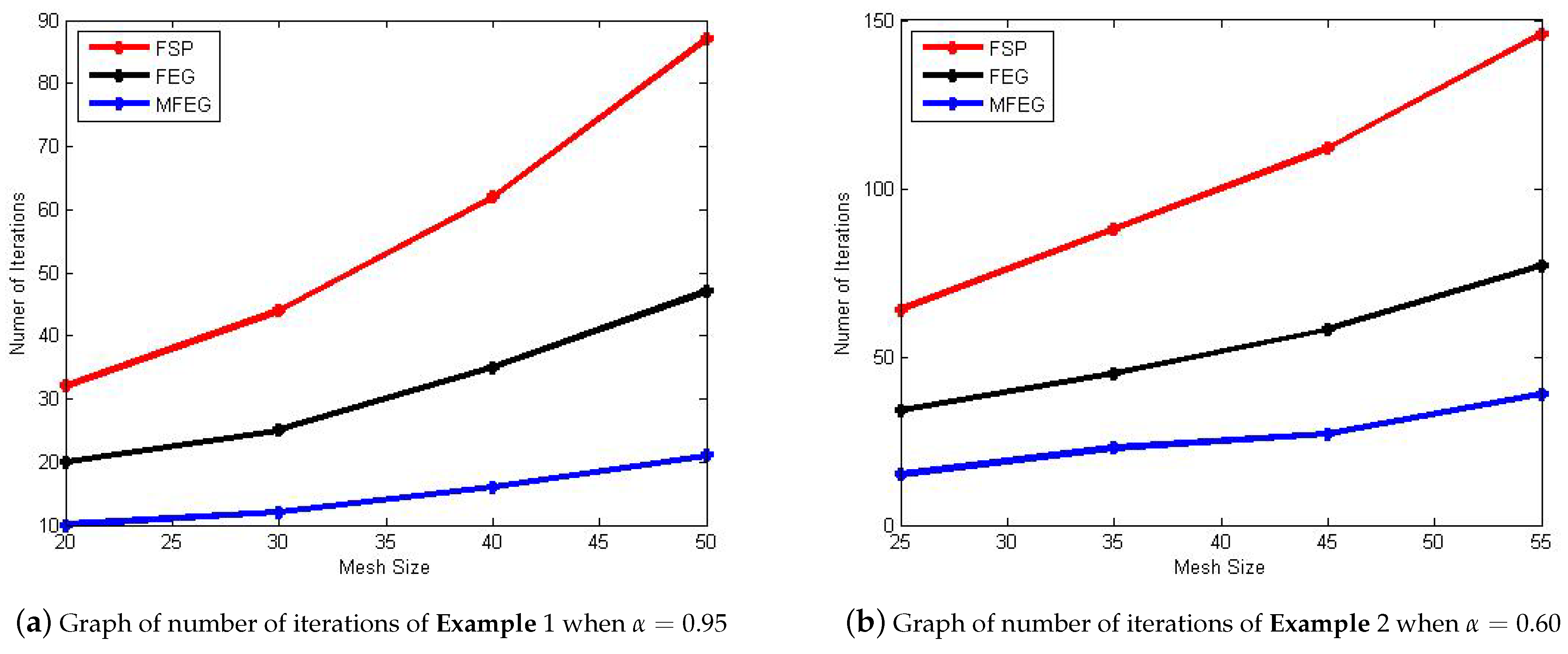
are obtained using the FSP, FEG, and MFEG iterative methods in terms of elapsed time (in seconds), number of iterations, average absolute error, and maximum absolute error. The fractional standard point (FSP) and fractional explicit group (FEG) iterative schemes are derived in [6] for 2D fractional telegraph equation. Graphs of execution time and iteration count are illustrated in Figure 1 and Figure 2 at various values of $\alpha$ for Example 1 and Example 2.

Example 1.

Consider the 2D time-fractional telegraph model together where the forcing term is defined by [6],

$$\frac{{\partial }^{2\alpha }\upsilon }{\partial t^{2\alpha }}+\frac{{\partial }^{\alpha }\upsilon }{\partial t^{\alpha }}+\upsilon =\frac{{\partial }^2\upsilon }{\partial x^2}+\frac{{\partial }^2\upsilon }{\partial y^2}-2sin\left(x\right)sin\left(y\right)(sin\left(t\right)-cos\left(t\right)).$$

Initial and boundary conditions are defined as follows:

$$\upsilon (x,y,0)={\psi }_1(x,y)=sin\left(x\right)sin\left(y\right),{\upsilon }_t(x,y,0)={\psi }_2(x,y)=0$$

$$\upsilon (0,y,t)=g_1(y,t)=0,\upsilon (1,y,t)=g_2(1,y,t)=cos\left(t\right)sin\left(1\right)sin\left(y\right)$$

$$\upsilon (x,0,t)=g_3(x,t)=0,\upsilon (x,1,t)=g_4(x,1,t)=cos\left(t\right)sin\left(x\right)sin\left(1\right).$$

The exact solution is $\upsilon (x,y,t)=sin\left(x\right)sin\left(y\right)cos\left(t\right).$

Example 2.

The 2D telegraph equation of fractional order is given by the following expression [6],

$$\frac{{\partial }^{2\alpha }\upsilon }{\partial t^{2\alpha }}+\frac{{\partial }^{\alpha }\upsilon }{\partial t^{\alpha }}+\upsilon =\frac{{\partial }^2\upsilon }{\partial x^2}+\frac{{\partial }^2\upsilon }{\partial y^2}-sinh\left(x\right)sinh\left(y\right)(2\alpha sin\left(t\right)-{\beta }^{2}cos\left(t\right)+3cos\left(t\right))$$

Let $\alpha =10$ and $\beta =5$, thus we have,

$$f(x,y,t)=sinh\left(x\right)sinh\left(y\right)(25cos(t)-20sin(t)-3cos(t\left)\right),$$

with the initial and boundary conditions:

$$\upsilon (x,y,0)={\psi }_1(x,y)=sinh\left(x\right)sinh\left(y\right),{\upsilon }_t(x,y,0)={\psi }_2(x,y)=0$$

$$\upsilon (0,y,t)=g_1(y,t)=0,\upsilon (1,y,t)=g_2(1,y,t)=cos\left(t\right)sinh\left(1\right)sinh\left(y\right)$$

$$\upsilon (x,0,t)=g_3(x,t)=0,\upsilon (x,1,t)=g_4(x,1,t)=cos\left(t\right)sinh\left(x\right)sinh\left(1\right).$$

The exact solution is $\upsilon (x,y,t)=cos\left(t\right)sinh\left(x\right)sinh\left(y\right).$

In Table 1 and Table 2, it is can be seen that execution time and iteration count decrease as value of $\alpha$ moves towards 2 by providing more accurate results.

The average absolute error and maximum absolute error are calculated by taking the absolute average and maximum absolute value of the column vector of errors, respectively. The maximum absolute error of the exact solution ${\mathrm{{\rm Y}}}_{i,j,k}$ and approximate solution ${\upsilon }_{i,j,k}$ is defined as follows:

$$e(\tau ,h)=\underset{2\le i\le M_x-2,2\le j\le M_y-2,0\le k\le N}{max}\{|{\mathrm{{\rm Y}}}_{i,j}^k-{\upsilon }_{i,j}^k|\}.$$

The temporal convergence order of the proposed method is defined as,

$${\gamma }_1-order\approx {log}_2\left(\frac{e(2\tau ,h)}{e(\tau ,h)}\right),$$

and the spatial convergence order of the proposed method is defined as,

$${\gamma }_2-order\approx {log}_2\left(\frac{e(\tau ,2h)}{e(\tau ,h)}\right)$$

Table 3. The maximum absolute error and temporal convergence order of MFEG iterative scheme at various values of $\alpha$ when $h=\frac{\pi }{200}$ subject to Example 1.

$\mathit{h}/\mathit{\tau }$		$\mathit{\alpha }$ = 0.65		$\mathit{\alpha }$ = 0.85
$\mathit{h}$	$\mathbf{\tau }$	$\mathit{e}(\mathbf{\tau },\mathit{h})$	${\mathbf{\gamma }}_{\mathbf{1}}$-order	$\mathit{e}(\mathbf{\tau },\mathit{h})$	${\mathbf{\gamma }}_{\mathbf{1}}$-order
$\frac{\pi }{200}$	1/50	7.6432 $\times {10}^{-4}$	-	5.6311 $\times {10}^{-4}$	-
	1/100	6.8721 $\times {10}^{-4}$	1.7432	4.6543 $\times {10}^{-4}$	1.9973
	1/150	8.9074 $\times {10}^{-5}$	1.7653	6.2953 $\times {10}^{-5}$	2.0016
	1/200	7.4285 $\times {10}^{-5}$	1.7862	5.8514 $\times {10}^{-5}$	2.0014

and

Table 4. The maximum absolute error and temporal convergence order of MFEG iterative scheme at various values of $\alpha$ when $h=\frac{\pi }{200}$ and subject to Example 2.

$\mathit{h}/\mathit{\tau }$		$\mathit{\alpha }$ = 0.70		$\mathit{\alpha }$ = 0.95
$\mathit{h}$	$\mathbf{\tau }$	$\mathit{e}(\mathbf{\tau },\mathit{h})$	${\mathbf{\gamma }}_{\mathbf{1}}$-order	$\mathit{e}(\mathbf{\tau },\mathit{h})$	${\mathbf{\gamma }}_{\mathbf{1}}$-order
$\frac{\pi }{200}$	1/100	4.6210 $\times {10}^{-4}$	-	5.6532 $\times {10}^{-4}$	-
	1/150	3.6778 $\times {10}^{-4}$	1.8045	4.7654 $\times {10}^{-4}$	2.0001
	1/200	2.9816 $\times {10}^{-4}$	1.8257	8.3680 $\times {10}^{-5}$	2.0008
	1/250	8.8243 $\times {10}^{-5}$	1.8466	7.6328 $\times {10}^{-5}$	2.0006

represent the values of maximum absolute error and temporal convergence order of MFEG iterative scheme at various values of $\alpha$ of Example 1 and Example 2. For fixed value of $h=\frac{\pi }{200}$ and different values of $\tau$, it is observed that MFEG iterative scheme generates $(3-2\alpha )$ temporal convergence order as shown in Table 3 and Table 4. Meanwhile, the

Table 5. The maximum absolute error and spatial convergence order of MFEG iterative scheme at various values of $\alpha$ when $\tau =0.001$ subject to Example 1.

$\mathit{h}/\mathit{\tau }$		$\mathit{\alpha }$ = 0.65		$\mathit{\alpha }$ = 0.85
$\mathit{h}$	$\mathbf{\tau }$	$\mathit{e}(\mathbf{\tau },\mathit{h})$	${\mathbf{\gamma }}_{\mathbf{2}}$-order	$\mathit{e}(\mathbf{\tau },\mathit{h})$	${\mathbf{\gamma }}_{\mathbf{2}}$-order
$\frac{1}{1000}$	$\frac{\pi }{20}$	3.6532 $\times {10}^{-3}$	-	2.5443 $\times {10}^{-3}$	-
	$\frac{\pi }{40}$	2.5321 $\times {10}^{-3}$	1.9264	1.7632 $\times {10}^{-3}$	2.0023
	$\frac{\pi }{60}$	5.7423 $\times {10}^{-4}$	1.9553	8.6432 $\times {10}^{-4}$	2.0019
	$\frac{\pi }{80}$	4.6234 $\times {10}^{-4}$	1.9823	7.7425 $\times {10}^{-4}$	2.0014

and

Table 6. The maximum absolute error and spatial convergence order of MFEG iterative scheme at various values of $\alpha$ when $\tau =0.001$ subject to Example 2.

$\mathit{h}/\mathit{\tau }$		$\mathit{\alpha }$ = 0.70		$\mathit{\alpha }$ = 0.95
$\mathit{h}$	$\mathbf{\tau }$	$\mathit{e}(\mathbf{\tau },\mathit{h})$	${\mathbf{\gamma }}_{\mathbf{2}}$-order	$\mathit{e}(\mathbf{\tau },\mathit{h})$	${\mathbf{\gamma }}_{\mathbf{2}}$-order
$\frac{1}{1000}$	$\frac{\pi }{25}$	3.6743 $\times {10}^{-3}$	-	7.6843 $\times {10}^{-4}$	-
	$\frac{\pi }{45}$	2.6743 $\times {10}^{-3}$	1.9043	6.7843 $\times {10}^{-4}$	2.0034
	$\frac{\pi }{65}$	9.9743 $\times {10}^{-4}$	1.9345	8.6743 $\times {10}^{-5}$	2.0028
	$\frac{\pi }{85}$	8.6743 $\times {10}^{-4}$	1.9584	7.5843 $\times {10}^{-5}$	2.0015

show the values of maximum absolute error and spatial convergence order of MFEG iterative scheme at various values of $\alpha$ of Example 1 and Example 2. For fixed value of $\tau =0.001$ and different values of h, it shows that MFEG iterative scheme gets second-order spatial accuracy as exposed in Table 5 and Table 6.

The ranges of percentages of MFEG method against FSP and FEG methods in terms of execution time and number of iterations of Example 1 at $\alpha =0.55$ and Example 2 at $\alpha =0.90$ are summarized in

Table 7. The percentages of MFEG method against FSP and FEG methods at $\alpha =0.55$ in Example 1.

Method	Execution Time (sec.)	Number of Iterations (Ite.)
FSP	(26.20–41.82)%	(22.30–32.60)%
FEG	(49.60–54.80)%	(45.40–56.30)%

and

Table 8. The percentages of MFEG method against FSP and FEG methods at $\alpha =0.90$ in Example 2.

Method	Execution Time (sec.)	Number of Iterations (Ite.)
FSP	(23.74–37.24)%	(21.64–31.90)%
FEG	(44.62–63.25)%	(47.20–65.25)%

, respectively.

Table 7 and Table 8 refer to the study of the percentages of MFEG method in term of the execution timings and number of iterations against FSP and FEG methods for solving the 2D fractional telegraph equation. Table 7 shows efficiency of execution of timings of MFEG method in Example 1 is about (26.0–42.0)% and (50.0–55.0)% of FSP and FEG methods while Table 8 indicates the execution of timings of MFEG method in Example 2 is merely about (24.0–37.0)% and (45.0–63.0)% of FSP and FEG method. The efficient percentages of MFEG iterative method for the number of iterations for both examples can also been seen in Table 7 and Table 8.

5. Conclusions

In this study, the unconditionally stable modified group relaxation method is constructed in the numerical solution of 2D hyperbolic telegraph equation. The MFEG method is derived from the standard Crank–Nicolson FD approximation with 2h grid spacing. It is observed that the suggested algorithm has more efficiency as compared to the other existing methods such as fractional standard point and fractional explicit group methods presented in [6]) in terms of number of iterations and elapsed CPU-timings. Amongst the schemes tested, the MFEG method is proven to require the least computational cost in terms of execution of timings. Moreover, it shown that the derived numerical temporal and spatial convergence order support our theoretical derivations. For a better convergence rate, in future, we will apply splitting-type preconditioner in block formulation applied to a class of group relaxation iterative methods for the numerical solution of various types of 2D time-fractional problems.

References

1. Lin, Y.H.; Liu, H.; Liu, X. Determining a nonlinear hyperbolic system with unknown sources and nonlinearity. arXiv 2021, arXiv:2107.10219. [Google Scholar]
2. Li, J.; Liu, H.; Ma, S. Determining a random Schrödinger operator: Both potential and source are random. Commun. Math. Phys. 2021, 381, 527–556. [Google Scholar] [CrossRef]
3. Liu, H.; Uhlmann, G. Determining both sound speed and internal source in thermo- and photo-acoustic tomography. Inverse Probl. 2015, 31, 105005. [Google Scholar] [CrossRef] [Green Version]
4. Cao, X.; Liu, H. Determining a fractional Helmholtz system with unknown source and medium parameter. Commun. Math. Sci. 2019, 17, 1861–1876. [Google Scholar] [CrossRef]
5. Cao, X.; Lin, Y.H.; Liu, H. Simultaneously recovering potentials and embedded obstacles for anisotropic fractional Schrödinger operators. Inverse Probl. Imaging 2019, 13, 197–210. [Google Scholar] [CrossRef] [Green Version]
6. Ali, A.; Ali, N.H.M. Explicit group iterative methods for the solution of two-dimensional time-fractional telegraph equation. In Proceedings of the 4th Innovation and Analytics Conference and Exhibition, AIP Conference Proceedings 2138, Sintok Kedah, Malaysia, 25–28 March 2019; pp. 1–6. [Google Scholar]
7. Ali, A.; Ali, N.H.M. On skewed grid point iterative method for solving 2D hyperbolic telegraph fractional differential equation. Adv. Differ. Equ. 2019, 303, 1–29. [Google Scholar] [CrossRef]
8. Ali, A.; Ali, N.H.M. New group fractional damped wave iterative solvers using Mathematica. In Proceedings of the International Conference on Mathematical Sciences and Technology, AIP Conference Proceedings 2184, Penang, Malaysia, 25–28 March 2019; pp. 1–10. [Google Scholar]
9. Ali, N.H.M.; Kew, L.M. New explicit group iterative methods in the solution of two-dimensional hyperbolic equations. J. Comput. Phys. 2012, 231, 6953–6968. [Google Scholar] [CrossRef]
10. Kew, L.M.; Ali, N.H.M. New explicit group iterative methods in the solution of three-dimensional hyperbolic telegraph equations. J. Comput. Phys. 2015, 294, 382–404. [Google Scholar] [CrossRef]
11. Evans, D.J.; Hasan, B. The numerical solution of the telegraph equation by the alternating group explicit (AGE) method. Int. J. Comput. Math. 2003, 80, 1289–1297. [Google Scholar] [CrossRef]
12. Gao, F.; Chi, C. Unconditionally stable difference schemes for a one-space-dimensional linear hyperbolic equation. Appl. Math. Comput. 2007, 187, 1272–1276. [Google Scholar] [CrossRef]
13. Youssef, M.I. Caputo–Katugampola fractional Volterra functional differential equations with a vanishing lag function. J. Nonlinear Sci. Appl. 2020, 13, 293–302. [Google Scholar] [CrossRef]
14. Asaduzzaman, M.; Kilicman, A.; Ali, M.Z. Presence and diversity of positive solutions for a Caputo–type fractional order nonlinear differential equation with an advanced argument. J. Math. Comput. Sci. 2020, 23, 230–244. [Google Scholar] [CrossRef]
15. Jassim, H.K.; Shareef, M.A. On approximate solutions for fractional system of differential equations with Caputo–Fabrizio fractional operator. J. Math. Comput. Sci. 2020, 23, 58–66. [Google Scholar] [CrossRef]
16. El-hady, E.S.; Öğrekçi, S. On Hyers-Ulam-Rassias stability of fractional differential equations with Caputo derivative. J. Math. Comput. Sci. 2020, 22, 325–332. [Google Scholar] [CrossRef]
17. Lai, J.; Liu, H. On a novel numerical scheme for Riesz fractional partial differential equations. Mathematics 2021, 9, 2014. [Google Scholar] [CrossRef]
18. Akram, T.; Abbas, M.; Ismail, A.I.; Ali, N.M.; Baleanu, D. Extended cubic B-splines in the numerical solution of time fractional telegraph equation. Adv. Differ. Equ. 2019, 365, 1–20. [Google Scholar] [CrossRef] [Green Version]
19. Akram, T.; Abbas, M.; Iqbal, A.; Baleanu, D.; Asad, J.H. Novel numerical approach based on modified extended cubic B-spline functions for solving non-linear time-fractional telegraph equation. Symmetry 2020, 12, 1154. [Google Scholar] [CrossRef]
20. Mohanty, R.K.; Jain, M.K. An unconditionally stable alternating direction implicit scheme for two space dimensional linear hyperbolic equation. Numer. Methods Partial Differ. Equ. 2001, 7, 684–688. [Google Scholar] [CrossRef]
21. Mohanty, R.K.; Jain, M.K.; Arora, U. An unconditionally stable {ADI} method for linear hyperbolic equation in three space dimensional. Int. J. Comput. Math. 2002, 79, 133–142. [Google Scholar] [CrossRef]
22. Mohanty, R.K. A new unconditionally stable diffierence schemes for the solution of multi-dimensional telegraphic equation. Int. J. Comput. Math. 2009, 86, 2061–2071. [Google Scholar] [CrossRef]
23. Dehghan, M.; Mehebbi, A. The combination of collocation finite difference and multigrid methods for solution of the two-dimensional wave equation. Numer. Methods Partial Differ. Equ. 2008, 24, 897–910. [Google Scholar] [CrossRef]
24. Dehghan, M.; Mehebbi, A. A high order implicit collocation method for the solution of two-dimensional linear hyperbolic equation. Numer. Methods Partial Differ. Equ. 2009, 25, 232–243. [Google Scholar] [CrossRef]
25. Saadatmandi, A.; Dehghan, M. Numerical solution of hyperbolic telegraph equation using the Chebyshev tau method. Numer. Methods Partial Differ. Equ. 2010, 26, 239–252. [Google Scholar] [CrossRef]
26. Dehghan, M.; Ghesmati, A. Combination of meshless local weak and strong {(MLWS)} forms to solve the two dimensional hyperbolic telegraph equation. Eng. Anal. Bound. Elem. 2010, 34, 324–336. [Google Scholar] [CrossRef]
27. Zhang, Y. A finite difference method for fractional partial differential equation. Appl. Math. Comput. 2009, 215, 524–529. [Google Scholar] [CrossRef]
28. Zhu, X.; Yuan, Z.; Wang, J.; Nie, Y.; Yang, Z. Finite element method for time-space-fractional schrodinger equation. Electron. J. Differ. Equ. 2017, 166, 1–18. [Google Scholar]
29. Katsikadelis, J.T. The boundary element method (BEM) for numerical solution of partial fractional differential equations. Comput. Math. Appl. 2011, 62, 891–901. [Google Scholar] [CrossRef] [Green Version]
30. Evans, D.J. Group explicit iterative methods for solving the large linear systems. Int. J. Comput. Math. 1985, 17, 81–108. [Google Scholar] [CrossRef]
31. Evans, D.J.; Yousif, W. Explicit group iterative methods for solving elliptic partial differential equations in 3-space dimensions. Int. J. Comput. Math. 1986, 18, 323–340. [Google Scholar] [CrossRef]
32. Evans, D.J.; Yousif, W. The explicit block relaxation method as grid smoother in the mutigrid V-cycle scheme. Int. J. Comput. Math. 1990, 34, 71–78. [Google Scholar] [CrossRef]
33. Evans, D.J.; Sahimi, M.S. The alternating group explicit iterative method AGE to solve the parabolic and hyperbolic partial differential equations. Annu. Rev. Numer. Fluid Mech. Heat Transf. 1988, 2, 383–389. [Google Scholar]
34. Abdullah, A.R. The four point explicit decoupled group EDG method: A fast Poisson solver. Int. J. Comput. Math. 1991, 38, 61–70. [Google Scholar] [CrossRef]
35. Yousif, W.S.; Evans, D.J. Explicit de-coupled group iterative methods anf their parallel implementations. Parallel Algorithms Appl. 1995, 7, 53–71. [Google Scholar] [CrossRef]
36. Ibrahim, A.; Abdullah, A.R. Solving the two-dimensional diffusion equation by the four point explicit decoupled EDG iterative method. Int. J. Comput. Math. 1995, 58, 253–256. [Google Scholar] [CrossRef]
37. Othman, M.; Abdullah, A.R. An efficient four points modified explicit group poisson solver. Int. J. Comput. Math. 2000, 76, 203–217. [Google Scholar] [CrossRef]
38. Sulaiman, J.; Othman, M.; Hasan, M.K. {MEGSOR} iterative schemes for the solution of {2D} elliptic {PDEs}. World Acad. Sci. Eng. Technol. 2010, 4, 418–424. [Google Scholar]
39. Balasim, A.T.; Ali, N.H.M. The Solution of {2D} Time fractional Diffusion Equation by the Fractional Modified Explicit Group Iterative Method. In Proceedings of the International Conference on Mathematics, Engineering and Industrial Applications, AIP Conference Proceedings 1775, Songkhla, Thailand, 24–26 July 2016; pp. 1–8. [Google Scholar]
40. Balasim, A.T.; Ali, N.H.M. Group Iterative Methods for the Solution of Two dimensional Time-fractional Diffusion Equation. In Proceedings of the Advances in Industrial and Applied Mathematics, AIP Conference Proceedings 1750, Johor Bahru, Malaysia, 24–26 November 2016; pp. 1–7. [Google Scholar]
41. Balasim, A.T.; Ali, N.H.M. New group iterative schemes in the numerical solution of the two-dimensional time fractional advection-diffusion equation. Cogent Math. 2017, 4, 1–19. [Google Scholar] [CrossRef]
Figure 1. Graphs of execution timings of point and group iterative schemes on various mesh sizes for Example 1 and Example 2.
Symmetry 13 02078 g001
Figure 2. Graphs of number of iterations of point and group iterative schemes on various mesh sizes for Example 1 and Example 2.
Symmetry 13 02078 g002