
A Generalized Two-Dimensional Index to Measure the Degree of Deviation from Double Symmetry in Square Contingency Tables


Abstract
:1. Introduction
2. Two-Dimensional Index to Measure Deviation from DS
3. Approximate Confidence Region for the Proposed Two-Dimensional Index
4. Examples
4.1. Utility of the Proposed Two-Dimensional Index
4.2. Example with Real Data
5. Concluding Remarks
Author Contributions
Funding
Institutional Review Board Statement
Informed Consent Statement
Data Availability Statement
Acknowledgments
Conflicts of Interest
Appendix A. Existing Index
Appendix B. Existing Index
References
- Bowker, A.H. A test for symmetry in contingency tables. J. Am. Stat. Assoc. 1948, 43, 572–574. [Google Scholar] [CrossRef] [PubMed]
- Bishop, Y.M.M.; Fienberg, S.E.; Holland, P.W. Discrete Multivariate Analysis: Theory and Practice; The MIT Press: Cambridge, MA, USA, 1975. [Google Scholar]
- Tan, T.K. Doubly Classified Model with R; Springer: Singapore, 2017. [Google Scholar]
- Agresti, A. An Introduction to Categorical Data Analysis, 3rd ed.; Wiley: Hoboken, NJ, USA, 2018. [Google Scholar]
- Wall, K.D.; Linert, G.A. A test for point-symmetry in J-dimensional contingency-cubes. Biom. J. 1976, 18, 259–264. [Google Scholar]
- Tomizawa, S. Double symmetry model and its decomposition in a square contingency table. J. Jpn. Stat. Soc. 1985, 15, 17–23. [Google Scholar]
- Tomizawa, S.; Seo, T.; Yamamoto, H. Power-divergence-type measure of departure from symmetry for square contingency tables that have nominal categories. J. Appl. Stat. 1998, 25, 387–398. [Google Scholar] [CrossRef]
- Tomizawa, S.; Yamamoto, K.; Tahata, K. An entropy measure of departure from point-symmetry for two-way contingency tables. Symmetry Cult. Sci. 2007, 18, 279–297. [Google Scholar]
- Yamamoto, K.; Komatsu, M.; Tomozawa, S. Measure of departure from double-symmetry for square contingency tables. J. Stat. Appl. 2010, 5, 105–118. [Google Scholar]
- Ando, S.; Tahata, K.; Tomizawa, S. A bivariate index vector for measuring departure from double symmetry in square contingency tables. Adv. Data Anal. Classif. 2019, 9, 519–529. [Google Scholar] [CrossRef] [Green Version]
- Cressie, N.A.C.; Read, T.R.C. Multinomial goodness-of-fit tests. J. R. Stat. Ser. B 1984, 46, 440–464. [Google Scholar] [CrossRef]
- Read, T.R.C.; Cressie, N.A.C. Goodness-of-Fit Statistics for Discrete Multivariate Data; Springer: New York, NY, USA, 1988. [Google Scholar]
- Agresti, A. Categorical Data Analysis, 3rd ed.; Wiley: Hoboken, NJ, USA, 2013. [Google Scholar]
- Andersen, E.B. Introduction to the Statistical Analysis of Categorical Data; Springer: Berlin, Germany, 1997. [Google Scholar]
- Tomizawa, S.; Miyamoto, N.; Iwamoto, M. Linear column-parameter symmetry model for square contingency tables: Application to decayed teeth data. Biom. Lett. 2006, 43, 91–98. [Google Scholar]
- Tomizawa, S.; Miyamoto, N.; Ohba, N. Improved approximate unbiased estimators of measures of asymmetry for square contingency tables. Adv. Appl. Stat. 2007, 7, 47–63. [Google Scholar]

| (a) | (b) | |||||||
| 137 | 71 | 948 | 986 | 801 | 247 | 132 | 104 | |
| 291 | 605 | 400 | 997 | 964 | 973 | 56 | 406 | |
| 1 | 450 | 268 | 361 | 85 | 952 | 333 | 393 | |
| 22 | 645 | 639 | 124 | 809 | 697 | 625 | 727 | |
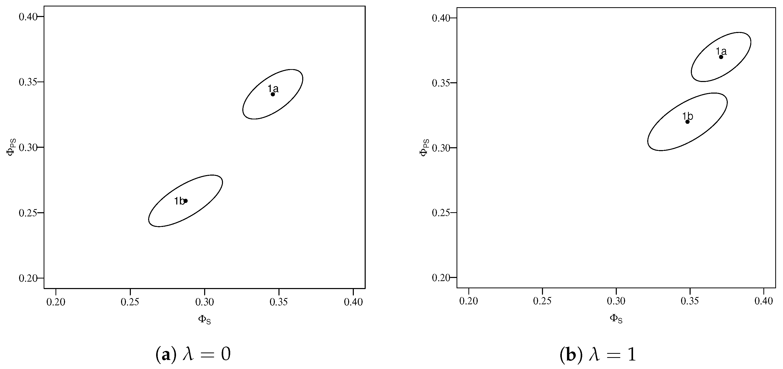
| (a) For Table 1a | |||||
| Index | Covariate Matrix | ||||
| 0 | 0.346 | 0.341 | 0.471 | 0.278 | 0.417 |
| 1 | 0.371 | 0.370 | 0.472 | 0.267 | 0.416 |
| (b) For Table 1b | |||||
| Index | Covariate Matrix | ||||
| 0 | 0.287 | 0.259 | 0.853 | 0.488 | 0.538 |
| 1 | 0.348 | 0.320 | 1.006 | 0.557 | 0.682 |
| (a) For prices | ||||
| Actual | ||||
| Forecast | Higher | No Change | Lower | Total |
| Higher | 209 | 169 | 6 | 384 |
| No change | 190 | 3073 | 184 | 3447 |
| Lower | 3 | 62 | 81 | 146 |
| Total | 402 | 3304 | 271 | 3977 |
| (b) For production | ||||
| Actual | ||||
| Forecast | Higher | No Change | Lower | Total |
| Higher | 532 | 394 | 69 | 995 |
| No change | 447 | 1727 | 334 | 2508 |
| Lower | 39 | 230 | 231 | 500 |
| Total | 1018 | 2351 | 634 | 4003 |
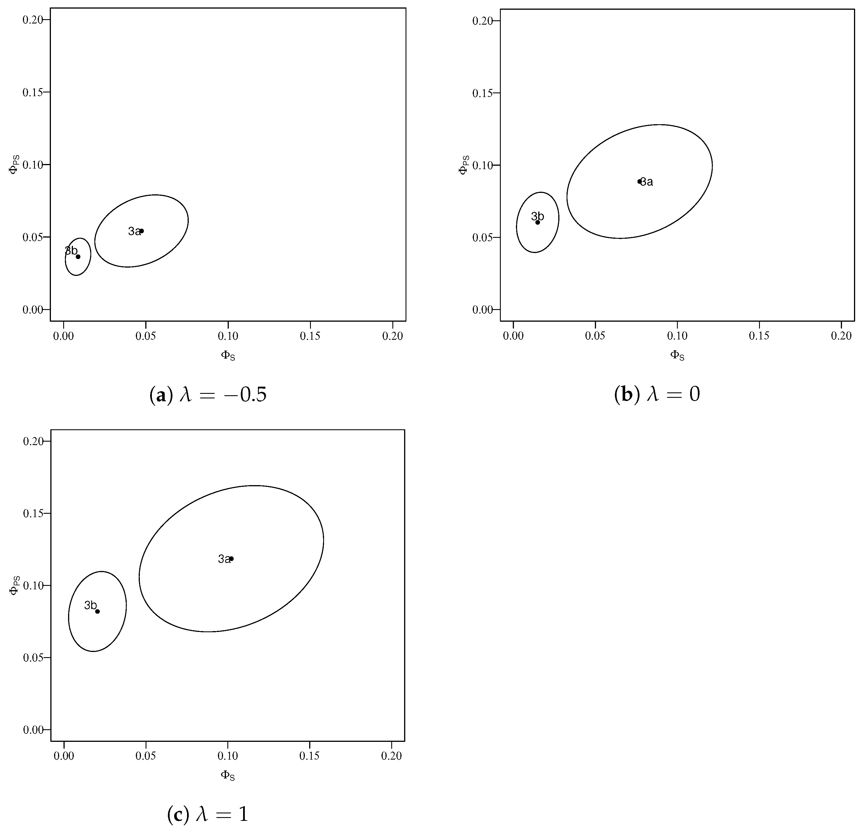
| (a) For Table 3a | |||||
| Index | Covariate Matrix | ||||
| −0.5 | 0.047 | 0.054 | 0.535 | 0.139 | 0.411 |
| 0 | 0.077 | 0.089 | 1.305 | 0.315 | 1.029 |
| 1 | 0.102 | 0.119 | 2.105 | 0.478 | 1.707 |
| (b) For Table 3b | |||||
| Index | Covariate Matrix | ||||
| −0.5 | 0.009 | 0.036 | 0.040 | 0.010 | 0.110 |
| 0 | 0.015 | 0.060 | 0.111 | 0.027 | 0.290 |
| 1 | 0.020 | 0.082 | 0.208 | 0.048 | 0.513 |
| (a) For female with left and right decayed teeth | ||||
| Right | ||||
| Left | 0 to 4 | 5 to 8 | 9 and above | Total |
| 0 to 4 | 103 | 45 | 1 | 149 |
| 5 to 8 | 35 | 84 | 33 | 152 |
| 9 and above | 3 | 17 | 42 | 62 |
| Total | 141 | 146 | 76 | 363 |
| (b) For female with lower and upper decayed data | ||||
| Upper | ||||
| Lower | 0 to 4 | 5 to 8 | 9 and above | Total |
| 0 to 4 | 97 | 62 | 15 | 174 |
| 5 to 8 | 20 | 63 | 75 | 158 |
| 9 and above | 2 | 6 | 23 | 31 |
| Total | 119 | 131 | 113 | 363 |
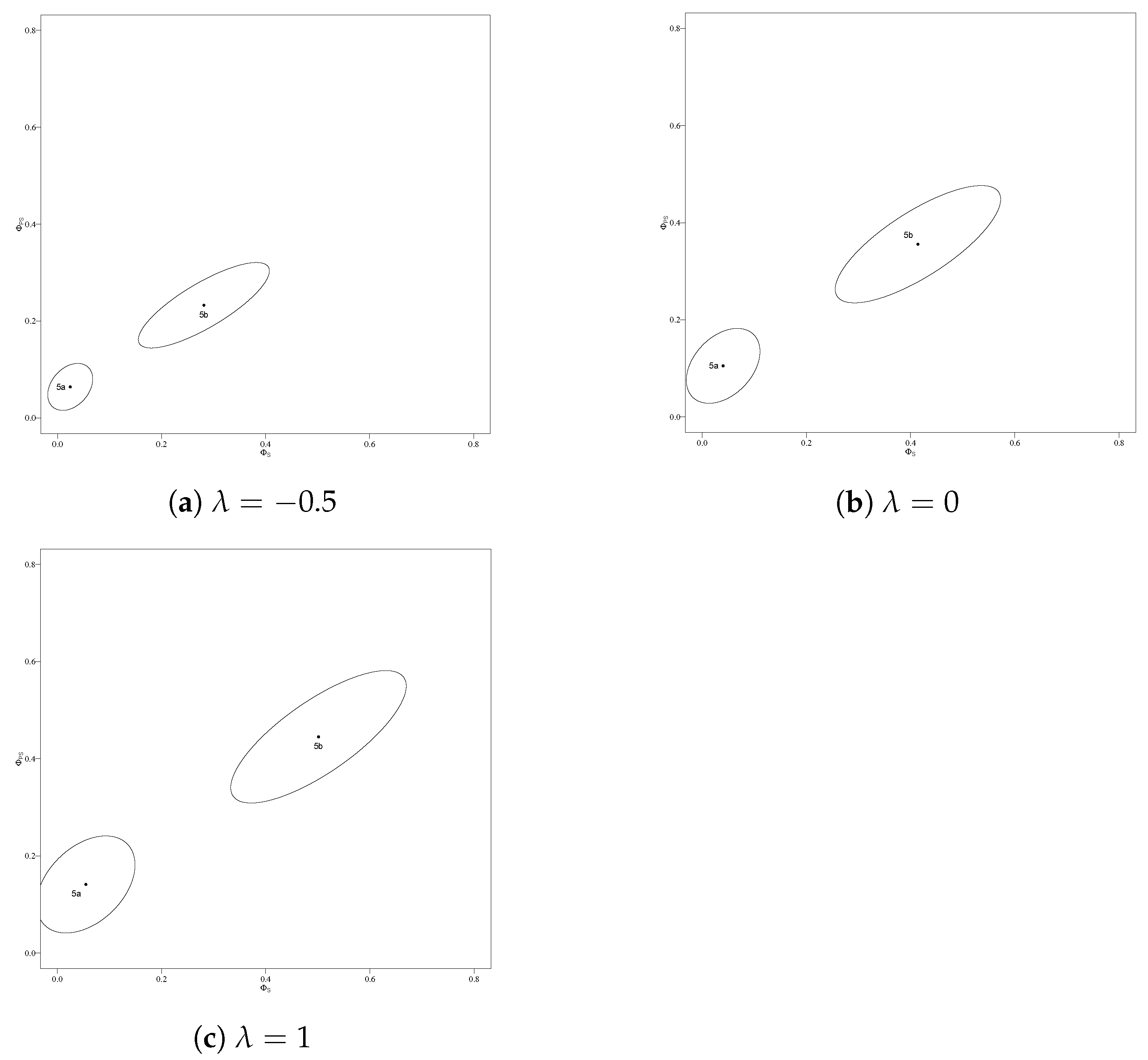
| (a) For Table 5a | |||||
| Index | Covariate Matrix | ||||
| −0.5 | 0.024 | 0.064 | 0.113 | 0.043 | 0.142 |
| 0 | 0.040 | 0.105 | 0.302 | 0.127 | 0.361 |
| 1 | 0.055 | 0.141 | 0.540 | 0.231 | 0.605 |
| (b) For Table 5b | |||||
| Index | Covariate Matrix | ||||
| −0.5 | 0.281 | 0.233 | 0.962 | 0.541 | 0.472 |
| 0 | 0.414 | 0.356 | 1.526 | 0.890 | 0.884 |
| 1 | 0.501 | 0.445 | 1.718 | 1.067 | 1.127 |
Publisher’s Note: MDPI stays neutral with regard to jurisdictional claims in published maps and institutional affiliations. |
© 2021 by the authors. Licensee MDPI, Basel, Switzerland. This article is an open access article distributed under the terms and conditions of the Creative Commons Attribution (CC BY) license (https://creativecommons.org/licenses/by/4.0/).
Share and Cite
Ando, S.; Hoshi, H.; Ishii, A.; Tomizawa, S. A Generalized Two-Dimensional Index to Measure the Degree of Deviation from Double Symmetry in Square Contingency Tables. Symmetry 2021, 13, 2067. https://doi.org/10.3390/sym13112067
Ando S, Hoshi H, Ishii A, Tomizawa S. A Generalized Two-Dimensional Index to Measure the Degree of Deviation from Double Symmetry in Square Contingency Tables. Symmetry. 2021; 13(11):2067. https://doi.org/10.3390/sym13112067
Chicago/Turabian StyleAndo, Shuji, Hikaru Hoshi, Aki Ishii, and Sadao Tomizawa. 2021. "A Generalized Two-Dimensional Index to Measure the Degree of Deviation from Double Symmetry in Square Contingency Tables" Symmetry 13, no. 11: 2067. https://doi.org/10.3390/sym13112067
APA StyleAndo, S., Hoshi, H., Ishii, A., & Tomizawa, S. (2021). A Generalized Two-Dimensional Index to Measure the Degree of Deviation from Double Symmetry in Square Contingency Tables. Symmetry, 13(11), 2067. https://doi.org/10.3390/sym13112067