Aboodh Transform Iterative Method for Solving Fractional Partial Differential Equation with Mittag–Leffler Kernel

Abstract

The major aim of this paper is the presentation of Aboodh transform of the Atangana–Baleanu fractional differential operator both in Caputo and Riemann–Liouville sense by using the connection between the Laplace transform and the Aboodh transform. Moreover, we aim to obtain the approximate series solutions for the time-fractional differential equations with an Atangana–Baleanu fractional differential operator in the Caputo sense using the Aboodh transform iterative method, which is the modification of the Aboodh transform by combining it with the new iterative method. The relation between the Laplace transform and the Aboodh transform is symmetrical. Some graphical illustrations are presented to describe the effect of the fractional order. The outcome reveals that Aboodh transform iterative method is easy to implement and adequately captures the behavior and the fractional effect of the fractional differential equation.

1. Introduction

The role of fractional differential operations in evaluating and simulating history dependent evolution models in physics and engineering cannot be over emphasized because of their properties [1,2,3,4,5]. Several definitions of fractional differential operator exist in literature. For extensive study on fractional derivative operators, refer to [6,7,8,9,10].

Recently, Atangana and Baleanu presented a new fractional differential operator which utilizes the Mittag–Leffler function as the kernel to replace the exponential function kernel of the Caputo-Fabrizo fractional differential operator [11,12]. This is performed with the purpose of introducing a non-local, non-singular kernel and to overcome the limitations of other fractional differential operators. For instance, the Riemman–Liouville fractional differential operator did not properly account for the initial condition, while the Caputo fractional differential operator was able to resolve this issue with the initial condition but was confronted with the limitation of singular kernel.

The use of an integral transform combined with analytical methods for the solution of fractional differential equations in the fast convergence series form is popular among researchers [13,14,15,16,17]. The concept of the Caputo–Fabrizio fractional derivative was extended to the model of HIV-1 infection of CD4${}^{+}$ T-cell using the homotopy analysis transform method in [18]. The fractional Caputo–Fabrizio derivative was utilized to introduce two types of new high order derivative with their existence solutions in [19]. The authors in [20] studied the Laplace transform, Sumudu transform, Fourier transform and Mellin transform of the Atangana–Baleanu fractional differential operator. Moreover, the Shehu transform was applied on the Atangana–Baleanu fractional derivative in [21], and some new related properties are established.

The novelty of this paper is the establishment of the Aboodh transform of the Atangana–Baleanu fractional differential operator both in the Caputo and Riemman–Liouville sense using the connection between the Laplace transform and the Aboodh transform. Moreover, we validate the Aboodh transform iterative method [4] for the solution of Atangana–Baleanu fractional differential equation.

We structure this paper as follows. Section 2 consist of the fundamental concept while, in Section 3, we discuss the basic idea of Aboodh transform iterative method. In Section 4, we validate the Aboodh transform iterative method for the solution of Atangana–Baleanu fractional differential equation and provide some concluding remarks in Section 5.

2. Preliminaries

In this section, some definitions, theorems and properties that will be useful in this paper is given.

Definition 1.

The Aboodh transform of a function Q(t) with exponential order over the class of functions [4]

$$\mathcal{C}=\{Q:|Q\left(t\right)|<B{e}^{p_j\left|t\right|},if t\in {(-1)}^j\times [0,\infty ),j=1,2;(B,p_1,p_2>0)\}$$

(1)

is written as

$$\mathcal{A}\left[Q\right(t\left)\right]=\mathcal{M}\left(\psi \right),$$

(2)

and defined as

$$\mathcal{A}\left[Q\left(t\right)\right]=\frac{1}{\psi }{\int }_0^{\infty }Q\left(t\right)e^{-\psi t}dt=\mathcal{M}\left(\psi \right),p_1\le \psi \le p_2.$$

(3)

Obviously, The Aboodh transform is linear as the Laplace transform.

Definition 2.

The inverse Aboodh transform of a function Q(t) is defined as [4].

$$Q\left(t\right)={\mathcal{A}}^{-1}\left[\mathcal{M}\left(\psi \right)\right].$$

(4)

Definition 3.

Let Q(t)$\in \mathcal{C},$ then the Laplace transform is defined by the following integral [22].

$$\mathcal{Q}\left(t\right)={\int }_0^{\infty }Q\left(t\right)e^{-st}dt.$$

(5)

The Laplace transform of Q(t) is written as follows.

$$\mathcal{L}\left[Q\right(t\left)\right]=\mathcal{Q}\left(s\right).$$

(6)

If ψ and s are unity, then Equations (3) and (5) are equal; hence, the relationships between the Aboodh transform and the Laplace transform are symmetrical.

Theorem 1

([23]). If Q(t) $\in \mathcal{C}$ with the Aboodh transform $\mathcal{A}$[Q(t)] and Laplace transform $\mathcal{L}$[Q(t)], then the following is the case.

$$\mathcal{M}\left(\psi \right)=\frac{1}{\psi }\mathcal{Q}\left(\psi \right).$$

(7)

Definition 4.

The Mittag–Leffler function is a special function that often occurs naturally in the solution of fractional order calculus, and it is defined as follows [24].

$$E_{\beta }\left(Z\right)=\sum _{\rho =0}^{\infty }\frac{Z^{\rho }}{\mathsf{\Gamma }(\rho \beta +1)},\beta ,Z\in \mathbb{C},\mathbb{R}e\left(\beta \right)\ge 0,$$

(8)

In generalized form [24], it is defined as follows.

$$E_{\beta ,\gamma }^{\mu }=\sum _{\rho =0}^{\infty }\frac{Z^{\rho }{\left(\mu \right)}_{\rho }}{\mathsf{\Gamma }(\gamma +\rho \beta )\rho !},\beta ,\gamma ,Z\in \mathbb{C},\mathbb{R}e\left(\beta \right)\ge 0,\mathbb{R}e\left(\gamma \right)\ge 0,$$

(9)

Moreover, we assume ${\left(\mu \right)}_{\rho }$ to be the Pochhammer’s symbol.

Definition 5.

Let Q $\in H^1(0,1)$ and $0<\beta <1,$ then the Atangana–Baleanu fractional derivative defined in the Caputo sense is given as follows [11].

$${}_0^{ABC}{D}_t^{\beta }Q\left(t\right)=\frac{N\left(\beta \right)}{1-\beta }{\int }_0^t{Q}^{{}^{\prime }}\left(x\right)E_{\beta }\left(\frac{-\beta {(t-x)}^{\beta }}{1-\beta }\right)dx.$$

(10)

Definition 6.

Let Q $\in H^1(0,1)$ and $0<\beta <1,$ then the Atangana–Baleanu fractional derivative defined in the Riemann–Liouville sense is given as follows [11].

$${}_0^{ABR}{D}_t^{\beta }Q\left(t\right)=\frac{N\left(\beta \right)}{1-\beta }\frac{d}{dt}{\int }_0^{t}Q\left(x\right)E_{\beta }\left(\frac{-\beta {(t-x)}^{\beta }}{1-\beta }\right)dx,$$

(11)

The normalization function N(β) > 0 satisfies the condition $N\left(0\right)=N\left(1\right)=1.$

Theorem 2

([11]). The Laplace transform of Atangana–Baleanu fractional derivative according to the Caputo sense is derived as follows:

$$\mathcal{L}\left[{}_0^{ABC}{D}_t^{\beta }Q\left(t\right)\right]=\frac{N\left(\beta \right)}{1-\beta }\times \frac{s^{\beta }F\left(s\right)-s^{\beta -1}f\left(0\right)}{s^{\beta }+\frac{\beta }{1-\beta }},$$

(12)

Moreover, the Laplace transform of Atangana–Baleanu fractional derivative according to the Riemann–Liouville sense is derived as follows.

$$\mathcal{L}\left[{}_0^{ABR}{D}_t^{\beta }Q\left(t\right)\right]=\frac{N\left(\beta \right)}{1-\beta }\times \frac{s^{\beta }F\left(s\right)}{s^{\beta }+\frac{\beta }{1-\beta }}.$$

(13)

Theorem 3.

If $\mathsf{\Omega },\beta \in \mathbb{C},$ with $\mathbb{R}e\left(\beta \right)>0,$ then the Aboodh transform of $E_{\beta }\left(\mathsf{\Omega }{t}^{\beta }\right)$ is derived as the following:

$$\mathcal{M}\left(E_{\beta }\left(\mathsf{\Omega }{t}^{\beta }\right)\right)=\frac{1}{{\psi }^2}{\left(1-\frac{\mathsf{\Omega }}{{\psi }^{\beta }}\right)}^{-1},$$

(14)

where $|\mathsf{\Omega }{\psi }^{-\beta }|<1.$

Proof of Theorem 3. 

Let us use the following Laplace transform formula:

$$\mathcal{L}\left[E_{\beta }\left(\mathsf{\Omega }{t}^{\beta }\right)\right]=\frac{1}{s}{(1-\mathsf{\Omega }{s}^{-\beta })}^{-1},$$

(15)

then by using Equation (7), we have the following.

$$\mathcal{M}\left(\psi \right)=\frac{1}{\psi }\mathcal{Q}\left(\psi \right)$$

$$=\frac{1}{\psi }\left(\frac{1}{\psi }{(1-\mathsf{\Omega }{\psi }^{-\beta })}^{-1}\right)$$

(16)

$$={\psi }^{-2}{(1-\mathsf{\Omega }{\psi }^{-\beta })}^{-1}.$$

(17)

□

Theorem 4.

Let $\beta ,$γ$\in \mathbb{C},$ with $\mathbb{R}e\left(\beta \right)>0,$$\mathbb{R}e\left(\gamma \right)>0,$ the Aboodh transform of $t^{\gamma -1}{E}_{\beta ,\mu }^{\mu }\left(\mathsf{\Omega }{t}^{\beta }\right)$ is derived as follows.

$$t^{\gamma -1}{E}_{\beta ,\mu }^{\mu }\left(\mathsf{\Omega }{t}^{\beta }\right)=\frac{1}{{\psi }^{\gamma +1}}{(1-\mathsf{\Omega }{\psi }^{-\beta })}^{-\mu },\left|\mathsf{\Omega }{\psi }^{-\beta }\right|<1.$$

(18)

Proof of Theorem 4. 

Let us use the Laplace transform formula:

$$\mathcal{L}\left[t^{\gamma -1}{E}_{\beta ,\gamma }^{\mu }\left(\mathsf{\Omega }{t}^{\beta }\right)\right]=s^{-\mu }{(1-\mathsf{\Omega }{s}^{-\beta })}^{-\mu },$$

(19)

then by using Equation (7), we have the following.

$$\mathcal{M}\left(t^{\gamma -1}{E}_{\beta ,\gamma }^{\mu }\left(\mathsf{\Omega }{t}^{\beta }\right)\right)=\frac{1}{\psi }\mathcal{Q}\left(\psi \right)$$

(20)

$$=\frac{1}{\psi }\left(\frac{1}{{\psi }^{\gamma }}{(1-\mathsf{\Omega }{\psi }^{-\beta })}^{-\mu }\right)$$

$$=\frac{1}{{\psi }^{\gamma +1}}{(1-\mathsf{\Omega }{\psi }^{\beta })}^{\mu }.$$

(21)

□

Theorem 5.

If $\mathcal{M}$(ψ) is the Aboodh transform of Q(t) $\in \mathcal{C}$ and $\mathcal{Q}$(s) is the Laplace transform of Q(t)$\in \mathcal{C},$ then the Aboodh transform of Atangana–Baleanu fractional derivative according to the Caputo sense is derived as follows.

$$\mathcal{M}\left({}_0^{ABC}{D}_t^{\beta }Q\left(t\right)\right)=\frac{N\left(\beta \right)(\mathcal{M}\left(\psi \right)-{\psi }^{-2}Q\left(0\right))}{1-\beta +\beta {\psi }^{-\beta }}.$$

(22)

Proof of Theorem 5. 

Using the relationship between the Aboodh transform and Laplace transform, we obtain the following.

$$\mathcal{M}\left({}_0^{ABC}{D}_t^{\beta }Q\left(t\right)\right)=\frac{1}{\psi }\left(\frac{N\left(\beta \right)}{1-\beta }\times \frac{{\psi }^{\beta }\mathcal{Q}\left(\psi \right)-{\psi }^{\beta -1}Q\left(0\right)}{{\psi }^{\beta }+\frac{\beta }{1-\beta }}\right)$$

$$={\psi }^{\beta }\left(N\left(\beta \right)\times \frac{\mathcal{M}\left(\psi \right)-{\psi }^{-2}Q\left(0\right)}{{\psi }^{\beta }(1-\beta +\beta {\psi }^{-\beta })}\right)$$

(23)

$$=N\left(\beta \right)\times \frac{(\mathcal{M}\left(\psi \right)-{\psi }^{-2}Q\left(0\right))}{1-\beta +\beta {\psi }^{-\beta }}.$$

□

Theorem 6.

Assume that $\mathcal{M}$(ψ) is the Aboodh transform of Q(t) $\in \mathcal{C}$ and $\mathcal{Q}\left(s\right)$ is the Laplace transform of Q(t) $\in \mathcal{C},$ then the Aboodh transform of Atangana–Baleanu fractional derivative according to the Riemann–Liouville sense is derived as follows.

$$\mathcal{M}\left({}_0^{ABR}{D}_t^{\beta }Q\left(t\right)\right)=\frac{N\left(\beta \right)\mathcal{M}\left(\psi \right)}{1-\beta +\beta {\psi }^{-\beta }}.$$

(24)

Proof of Theorem 6. 

By using the relationship between the Aboodh transform transform and the Laplace transform, we obtain the following.

$$\mathcal{M}\left({}_0^{ABR}{D}_t^{\beta }Q\left(t\right)\right)=\frac{1}{\psi }\left(\frac{N\left(\beta \right)}{1-\beta }\times \frac{{\psi }^{\beta }\mathcal{Q}\left(\psi \right)}{{\psi }^{\beta }+\frac{\beta }{1-\beta }}\right)$$

$$=\frac{1}{\psi }\left(\frac{N\left(\beta \right)\mathcal{Q}\left(\psi \right)}{1-\beta +\beta {\psi }^{-\beta }}\right)$$

(25)

$$=\frac{N\left(\beta \right)\mathcal{M}\left(\psi \right)}{1-\beta +\beta {\psi }^{-\beta }}.$$

□

3. Aboodh Transform Iterative Method

In this section, we consider the fundamental solution of the initial value problem using the Aboodh transform iterative method. This iterative method is a combination of the new iterative method introduced by Daftardar–Gejji and Jafari [25] with the Aboodh transform which is a modification of the Laplace transform [4].

Basic Idea of Aboodh Transform Iterative Method

Consider the fractional differential equation of the following:

$${}_0^{ABC}{D}_t^{\beta }Q(x,t)=\mathcal{R}\left(Q(x,t)\right)+\mathcal{F}\left(Q(x,t)\right)+\mathsf{\Phi }(x,t),0<\beta \le 1,$$

(26)

that is subject to the following initial condition.

$$Q(x,0)=Q_0\left(x\right),$$

(27)

${}_0^{ABC}{D}_t^{\beta }$ is the Atangana–Baleanu fractional differential operator, $\mathsf{\Phi }(x,t)$ is the source term, $\mathcal{R}$ and $\mathcal{F}$ are the linear and non-linear operators. Using the Aboodh transform on both sides of Equation (26) with the initial condition, we obtain the following.

$$\begin{array}{c}\hfill \mathcal{A}\left[Q(x,t)\right]=\frac{1-\beta +\beta {\psi }^{-\beta }}{N\left(\beta \right)}\left(\frac{N\left(\beta \right){\psi }^{-2}Q(x,0)}{1-\beta +\beta {\psi }^{-\beta }}+\mathcal{A}\left[\mathcal{R}\left(Q\right(x,t\left)\right)+\mathcal{F}\left(Q\right(x,t\left)\right)+\mathsf{\Phi }(x,t)\right]\right),\end{array}$$

(28)

By simplifying further and taking the inverse Aboodh transform, we obtain the following.

$$Q(x,t)={\mathcal{A}}^{-1}\left[\frac{1-\beta +\beta {\psi }^{-\beta }}{N\left(\beta \right)}\left(\frac{N\left(\beta \right){\psi }^{-2}Q(x,0)}{1-\beta +\beta {\psi }^{-\beta }}+\mathcal{A}\left[\mathsf{\Phi }(x,t)\right]+\mathcal{A}\left[\mathcal{R}\left(Q\right(x,t\left)\right)+\mathcal{F}\left(Q\right(x,t\left)\right)\right]\right)\right].$$

(29)

The non-linear term in Equation (29) can be decompose as follows [25].

$$\mathcal{F}\left(Q\right(x,t\left)\right)=\mathcal{F}\left(\sum _{q=0}^{\infty }{Q}_q(x,t)\right)$$

$$=\mathcal{F}\left(Q_0(x,t)\right)+\sum _{q=1}^{\infty }\left\{\mathcal{F}\left(\sum _{j=0}^q{Q}_q(x,t)\right)-\mathcal{F}\left(\sum _{j=0}^{q-1}{Q}_q(x,t)\right)\right\}.$$

(30)

Now, we define the k-th order approximate series as the following.

$${\mathcal{Q}}^{\left(k\right)}(x,t)=\sum _{m=0}^k{Q}_m(x,t)$$

$$=Q_0(x,t)+Q_1(x,t)+Q_2(x,t)+\cdots +Q_k(x,t),k\in N.$$

(31)

Assume that the solution of Equation (26) is in a series form given as follow.

$$Q(x,t)=\underset{k\to \infty }{lim}{\mathcal{Q}}^{\left(k\right)}(x,t)=\sum _{m=0}^{\infty }{Q}_m(x,t),$$

(32)

Then, substituting Equations (31) and (30) into Equation (29), we obtain the following.

$$\begin{array}{c}\sum _{q=0}^{\infty }{Q}_q(x,t)=\hfill \\ {\mathcal{A}}^{-1}\left[\frac{1-\beta +\beta {\psi }^{-\beta }}{N\left(\beta \right)}\left(\frac{N\left(\beta \right){\psi }^{-2}Q(x,0)}{1-\beta +\beta {\psi }^{\beta }}+\mathsf{\Phi }(x,t)+\mathcal{A}\left[\mathcal{R}\left(Q_0(x,t)\right)+\mathcal{F}\left(Q_0(x,t)\right)\right]\right)\right]+\\ \hfill {\mathcal{A}}^{-1}\left[\frac{1-\beta +\beta {\psi }^{-\beta }}{N\left(\beta \right)}\left(\mathcal{A}\left[\sum _{q=1}^{\infty }\left(\mathcal{R}\left(Q_q(x,t)\right)+\left\{\mathcal{F}\left(\sum _{j=0}^q(x,t)\right)-\mathcal{F}\left(\sum _{j=0}^{q-1}{Q}_q(x,t)\right)\right\}\right)\right]\right)\right].\end{array}$$

(33)

From Equation (33), we define the following iterations.

$$Q_0(x,t)={\mathcal{A}}^{-1}\left[\frac{1-\beta +\beta {\psi }^{-\beta }}{N\left(\beta \right)}\left(\frac{N\left(\beta \right){\psi }^{-2}Q(x,0)}{1-\beta +\beta {\psi }^{\beta }}+\mathsf{\Phi }(x,t)\right)\right],$$

(34)

$$Q_1(x,t)={\mathcal{A}}^{-1}\left[\frac{1-\beta +\beta {\psi }^{-\beta }}{N(\beta )}\left(\mathcal{A}\left[\mathcal{R}\left(Q_0(x,t)\right)+\mathcal{F}\left(Q_0(x,t)\right)\right]\right)\right],$$

(35)

$$⋮$$

$$\begin{array}{c}{Q}_{q+1}=\hfill \\ {\mathcal{A}}^{-1}\left[\frac{1-\beta +\beta {\psi }^{-\beta }}{N\left(\beta \right)}\left(\mathcal{A}\left[\sum _{q=1}^{\infty }\left(\mathcal{R}\left(Q_q(x,t)\right)+\left\{\mathcal{F}\left(\sum _{j=0}^q(x,t)\right)-\mathcal{F}\left(\sum _{j=0}^{q-1}{Q}_q(x,t)\right)\right\}\right)\right]\right)\right],\\ \hfill q=1,2,\cdots \end{array}$$

(36)

Convergence Analysis

We establish the convergence analysis of the series in Equation (32) here.

Theorem 7.

Suppose that the nonlinear operator and the linear operator are from the Banach space X relative to itself, and Q(x,t) is analytic about t. Then the infinite series defined in Equation (32) computed by Equations (34), (35),…, (36) converges to the solution of Equation (26) if $0<\rho \le 1$, where ρ is a nonnegative real number.

Proof. 

Let $\left\{S_q\right\}$ be the partial sum of the series in Equation (32). Then, we have to show that $\left\{S_q\right\}$ is Cauchy sequence in X.

Consider the following.

$$\left|\right|S_{q+1}(x,t)-S_q(x,t)\left|\right|=\left|\right|Q_{q+1}(x,t)\left|\right|\le \rho \left|\right|Q_q(x,t)\left|\right|\le {\rho }^2\left|\right|Q_{q-1}(x,t)\left|\right|\le \cdots \le {\rho }^{q+1}\left|\right|Q_0(x,t)\left|\right|.$$

For every $q,r\in N$ ($r\le q$), the following is the case.

$$\left|\right|S_q-S_r\left|\right|=\left|\right|(S_q-S_{q-1})+(S_{q-1}-S_{q-2})+\cdots +(S_{r+1}-S_r)\left|\right|$$

$$\le \left|\right|(S_q-S_{q-1})\left|\right|+\left|\right|(S_{q-1}-S_{q-2})\left|\right|+\cdots +\left|\right|(S_{r+1}-S_r)\left|\right|$$

$$\le ({\rho }^q+{\rho }^{q+1}+\cdots +{\rho }^{r+1})\left|\right|Q_0(x,t)\left|\right|$$

$$\le {\rho }^{r+1}({\rho }^{q-r-1}+{\rho }^{q-r-2}+\rho +1)\left|\right|Q_0(x,t)\left|\right|$$

$$\le {\rho }^{r+1}\left(\frac{1-{\rho }^{q-r}}{1-\rho }\right)\left|\right|Q_0(x,t)\left|\right|.$$

However, $0<\rho \le 1$; therefore, $\left|\right|S_q-S_r\left|\right|=0$. Hence, the sequence $\left\{S_q\right\}$ is a Cauchy sequence. □

4. Applications

Here, we consider five distinct differential equations with the Atangana–Baleanu fractional derivative in order to validate the application of the scheme with different initial conditions.

Example 1.

Consider Equation (26) as the time-fractional gas dynamics equation:

$${}_0^{ABC}{D}_t^{\beta }Q+\frac{1}{2}{\left(Q^2\right)}_x-Q\left(1-Q\right)=0,0<\beta \le 1.$$

(37)

with the following initial condition.

$$\begin{array}{cc}\hfill & Q_0\left(x\right)=e^{-x}.\hfill \end{array}$$

(38)

From Equations (37) and (38), we set the following.

$$\begin{array}{ccc}\hfill & \mathcal{R}\left(Q(x,t)\right)=-Q,\hfill & \\ \hfill & \mathcal{F}\left(Q(x,t)\right)=\frac{1}{2}{\left(Q^2\right)}_x+Q^2,\hfill & \\ \hfill & Q_0(x,0)=e^{-x}.\hfill \end{array}$$

By employing the iteration procedure described in Section 3, we obtain the following.

$$Q_0={\mathcal{A}}^{-1}\left[\frac{1-\beta +\beta {\psi }^{-\beta }}{N\left(\beta \right)}\left(\frac{N\left(\beta \right){\psi }^{-2}\mathcal{Q}(x,0)}{1-\beta +\beta {\psi }^{-\beta }}\right)\right],0<\beta \le 1$$

$$={\mathcal{A}}^{-1}\left[{\psi }^{-2}Q(x,0)\right]$$

(39)

$$={\mathcal{A}}^{-1}\left[{\psi }^{-2}{e}^{-x}\right]$$

$$=e^{-x},$$

$$Q_1={\mathcal{A}}^{-1}\left[\frac{1-\beta +\beta {\psi }^{-\beta }}{N\left(\beta \right)}\left(\mathcal{A}\left[\mathcal{R}\left(Q_0(x,t)\right)+\mathcal{F}\left(Q_0(x,t)\right)\right]\right)\right]$$

$$={\mathcal{A}}^{-1}\left[\frac{1-\beta +\beta {\psi }^{-\beta }}{N\left(\beta \right)}\left(\mathcal{A}\left[Q_0-\left(\frac{1}{2}{\left(Q_0^2\right)}_x+Q_0^2\right)\right]\right)\right]$$

(40)

$$={\mathcal{A}}^{-1}\left[\left(\frac{(1-\beta ){\psi }^{\beta }+\beta }{N\left(\beta \right)}\right)\frac{e^{-x}}{{\psi }^{2+\beta }}\right]$$

$$=\left(\frac{(1-\beta ){\psi }^{\beta }+\beta }{N\left(\beta \right)}\right)\frac{e^{-x}}{\mathsf{\Gamma }(\beta +1)},$$

$$\begin{array}{c}{Q}_2={\mathcal{A}}^{-1}\left[\frac{1-\beta +\beta {\psi }^{-\beta }}{N\left(\beta \right)}\left(\mathcal{A}\left[\mathcal{R}\left(Q_1(x,t)\right)+\left\{\mathcal{F}\left(Q_0(x,t)+Q_1(x,t)\right)-\mathcal{F}\left(Q_0(x,t)\right)\right\}\right]\right)\right]\\ ={\mathcal{A}}^{-1}\left[\frac{1-\beta +\beta {\psi }^{-\beta }}{N\left(\beta \right)}\left(\mathcal{A}\left[Q_1+\left\{\left(\frac{1}{2}{\left({(Q_0+Q_1)}^2\right)}_x+{(Q_0+Q_1)}^2\right)+\left(\frac{1}{2}{\left(Q_0^2\right)}_x+Q_0^2\right)\right\}\right]\right)\right]\\ ={\mathcal{A}}^{-1}\left[{\left(\frac{(1-\beta ){\psi }^{\beta }+\beta }{N\left(\beta \right)}\right)}^2\frac{e^{-x}}{{\psi }^{2+2\beta }}\right]\\ ={\left(\frac{(1-\beta ){\psi }^{\beta }+\beta }{N\left(\beta \right)}\right)}^2\frac{e^{-x}}{\mathsf{\Gamma }(2\beta +1),}\end{array}$$

(41)

$$⋮$$

$$\begin{array}{c}{Q}_k={\mathcal{A}}^{-1}\left[\frac{1-\beta +\beta {\psi }^{-\beta }}{N\left(\beta \right)}\left(\mathcal{A}\left[\mathcal{R}\left(Q_{k-1}(x,t)\right)+\left\{\mathcal{F}\left(\sum _{j=0}^k{Q}_j(x,t)\right)+\mathcal{F}\left(\sum _{j=0}^{k-1}{Q}_j(x,t)\right)\right\}\right]\right)\right]\\ ={\mathcal{A}}^{-1}\left[\frac{1-\beta +\beta {\psi }^{-\beta }}{N\left(\beta \right)}\left(\mathcal{A}\left[{\left(\frac{(1-\beta ){\psi }^{\beta }+\beta }{N\left(\beta \right)}\right)}^{k-1}{Q}_{k-1}(x,t)\right]\right)\right]\\ ={\mathcal{A}}^{-1}\left[{\left(\frac{(1-\beta ){\psi }^{\beta }+\beta }{N\left(\beta \right)}\right)}^k\frac{e^{-x}}{{\psi }^{2+k\beta }}\right]\\ ={\left(\frac{(1-\beta ){\psi }^{\beta }+\beta }{N\left(\beta \right)}\right)}^k\frac{e^{-x}{t}^{k\beta }}{\mathsf{\Gamma }(k\beta +1)}.\end{array}$$

(42)

We derived the k-th approximate series solution as follows:

$${\mathcal{Q}}^{\left(k\right)}(x,t)=\sum _{m=0}^k{Q}_m(x,t)=Q_0(x,0)+Q_1(x,t)+Q_2(x,t)+\cdots +Q_k(x,t)$$

$$=e^{-x}\left(1+\left(\frac{(1-\beta ){\psi }^{\beta }+\beta }{N\left(\beta \right)}\right)\frac{t^{\beta }}{\mathsf{\Gamma }(\beta +1)}+\cdots +{\left(\frac{(1-\beta ){\psi }^{\beta }+\beta }{N\left(\beta \right)}\right)}^k\frac{t^{k\beta }}{\mathsf{\Gamma }(k\beta +1)}\right)$$

$$=e^{-x}\sum _{m=0}^k{\left(\frac{(1-\beta ){\psi }^{\beta }+\beta }{N\left(\beta \right)}\right)}^m\frac{t^{m\beta }}{\mathsf{\Gamma }(m\beta +1)},$$

(43)

when $k\to \infty$, the k-th order approximate series results in the exact solution.

$$Q(x,t)=\underset{k\to \infty }{lim}{\mathcal{Q}}^{\left(k\right)}(x,t)$$

$$=e^{-x}\underset{k\to \infty }{lim}\sum _{m=0}^k{\left(\frac{(1-\beta ){\psi }^{\beta }+\beta }{N\left(\beta \right)}\right)}^m\frac{t^{m\beta }}{\mathsf{\Gamma }(m\beta +1)}$$

(44)

$$=e^{-x}{E}_{\beta }\left(\frac{((1-\beta ){\psi }^{\beta }+\beta )t^{\beta }}{N\left(\beta \right)}\right).$$

When $\beta =1,$ we obtain the exact solution as follows:

$$=e^{-x}{E}_1\left(t\right)$$

$$=e^{t-x},$$

(45)

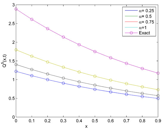
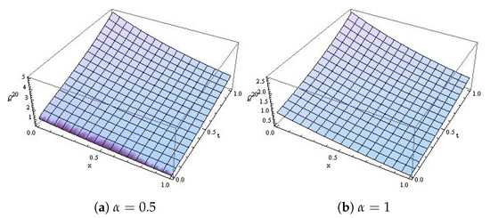
which is the exact solution obtained in [2]. Figure 1 reveals the effect of α and the natural behavior of the model at distinct values of α. Moreover, Figure 2a,b is the surface plot at $\alpha =0.5$ and 1, respectively.

Figure 1. Comparison plot of the exact and approximate solutions for Example 1.

Figure 2. The surface plot for Example 1.

Example 2.

Consider Equation (26) as the one dimensional time-fractional biological population model according to Verhulst law [26]:

$${}_0^{ABC}{D}_t^{\beta }Q={\left(Q^2\right)}_{xx}+Q\left(1-\frac{4}{25}Q\right),t>0,0<\beta \le 1,$$

(46)

with the following initial condition.

$$\begin{array}{cc}\hfill & Q_0\left(x\right)=e^{\frac{1}{5}}.\hfill \end{array}$$

(47)

From Equations (46) and (47), we set the following.

$$\begin{array}{ccc}& \mathcal{R}\left(Q(x,t)\right)=Q,\hfill & \\ & \mathcal{F}\left(Q(x,t)\right)={\left(Q^2\right)}_{xx}-\frac{4}{25}{Q}^2,\hfill & \\ & Q_0(x,0)=e^{\frac{1}{5}x}.\hfill \end{array}$$

By employing the iteration procedure described in Section 3, we obtain the following.

$$Q_0={\mathcal{A}}^{-1}\left[\frac{1-\beta +\beta {\psi }^{-\beta }}{N\left(\beta \right)}\left(\frac{N\left(\beta \right){\psi }^{-2}\mathcal{Q}(x,0)}{1-\beta +\beta {\psi }^{-\beta }}\right)\right],0<\beta \le 1$$

$$={\mathcal{A}}^{-1}\left[{\psi }^{-2}Q(x,0)\right]$$

(48)

$$={\mathcal{A}}^{-1}\left[{\psi }^{-2}{e}^{\frac{1}{5}x}\right]$$

$$=e^{\frac{1}{5}x},$$

$$Q_1={\mathcal{A}}^{-1}\left[\frac{1-\beta +\beta {\psi }^{-\beta }}{N\left(\beta \right)}\left(\mathcal{A}\left[\mathcal{R}\left(Q_0(x,t)\right)+\mathcal{F}\left(Q_0(x,t)\right)\right]\right)\right]$$

$$={\mathcal{A}}^{-1}\left[\frac{1-\beta +\beta {\psi }^{-\beta }}{N\left(\beta \right)}\left(\mathcal{A}\left[Q_0+{\left(Q_0^2\right)}_{xx}-{\displaystyle \frac{4}{25}}{Q}_0^2\right]\right)\right]$$

$$={\mathcal{A}}^{-1}\left[\left(\frac{(1-\beta ){\psi }^{\beta }+\beta }{N\left(\beta \right)}\right)\frac{e^{\frac{x}{5}}}{{\psi }^{2+\beta }}\right]$$

(49)

$$=\left(\frac{(1-\beta ){\psi }^{\beta }+\beta }{N\left(\beta \right)}\right)\frac{e^{\frac{x}{5}}{t}^{\beta }}{\mathsf{\Gamma }(\beta +1)},$$

$$Q_2={\mathcal{A}}^{-1}\left[\frac{1-\beta +\beta {\psi }^{-\beta }}{N\left(\beta \right)}\left(\mathcal{A}\left[\mathcal{R}\left(Q_1(x,t)\right)+\left\{\mathcal{F}\left(Q_0(x,t)+Q_1(x,t)\right)-\mathcal{F}\left(Q_0(x,t)\right)\right\}\right]\right)\right]$$

$$\begin{array}{c}={\mathcal{A}}^{-1}\left[\frac{1-\beta +\beta {\psi }^{-\beta }}{N\left(\beta \right)}\left(\mathcal{A}\left[Q_1+\left\{{\left({(Q_0+Q_1)}^2\right)}_{xx}-\frac{4}{25}{(Q_0+Q_1)}^2-{\left(Q_0^2\right)}_{xx}+\frac{4}{25}{Q}_0^2\right\}\right]\right)\right]\\ ={\mathcal{A}}^{-1}\left[{\left(\frac{(1-\beta ){\psi }^{\beta }+\beta }{N\left(\beta \right)}\right)}^2\frac{e^{\frac{x}{5}}}{{\psi }^{2+2\beta }}\right]\\ ={\left(\frac{(1-\beta ){\psi }^{\beta }+\beta }{N\left(\beta \right)}\right)}^2\frac{e^{\frac{x}{5}}{t}^{2\beta }}{\mathsf{\Gamma }(2\beta +1),}\end{array}$$

(50)

$$⋮$$

$$\begin{array}{c}{Q}_k={\mathcal{A}}^{-1}\left[\frac{1-\beta +\beta {\psi }^{-\beta }}{N\left(\beta \right)}\left(\mathcal{A}\left[\mathcal{R}\left(Q_{k-1}(x,t)\right)+\left\{\mathcal{F}\left(\sum _{j=0}^k{Q}_j(x,t)\right)+\mathcal{F}\left(\sum _{j=0}^{k-1}{Q}_j(x,t)\right)\right\}\right]\right)\right]\\ ={\mathcal{A}}^{-1}\left[\frac{1-\beta +\beta {\psi }^{-\beta }}{N\left(\beta \right)}\left(\mathcal{A}\left[{\left(\frac{(1-\beta ){\psi }^{\beta }+\beta }{N\left(\beta \right)}\right)}^{k-1}{Q}_{k-1}(x,t)\right]\right)\right]\\ ={\mathcal{A}}^{-1}\left[{\left(\frac{(1-\beta ){\psi }^{\beta }+\beta }{N\left(\beta \right)}\right)}^k\frac{e^{\frac{x}{5}}}{{\psi }^{2+k\beta }}\right]\\ ={\left(\frac{(1-\beta ){\psi }^{\beta }+\beta }{N\left(\beta \right)}\right)}^k\frac{e^{\frac{x}{5}}{t}^{k\beta }}{\mathsf{\Gamma }(k\beta +1)}.\end{array}$$

(51)

We derived the k-th approximate series solution as the following:

$$\begin{array}{c}{\mathcal{Q}}^{\left(k\right)}(x,t)=\sum _{m=0}^k{Q}_m(x,t)=Q_0(x,0)+Q_1(x,t)+Q_2(x,t)+\cdots +Q_k(x,t)\\ =e^{\frac{x}{5}}\left(1+\left(\frac{(1-\beta ){\psi }^{\beta }+\beta }{N\left(\beta \right)}\right)\frac{t^{\beta }}{\mathsf{\Gamma }(\beta +1)}+\cdots +{\left(\frac{(1-\beta ){\psi }^{\beta }+\beta }{N\left(\beta \right)}\right)}^k\frac{t^{k\beta }}{\mathsf{\Gamma }(k\beta +1)}\right)\\ =e^{\frac{x}{5}}\sum _{m=0}^k{\left(\frac{(1-\beta ){\psi }^{\beta }+\beta }{N\left(\beta \right)}\right)}^m\frac{t^{m\beta }}{\mathsf{\Gamma }(m\beta +1)},\end{array}$$

(52)

when $k\to \infty$, the k-th order approximate series results in the exact solution.

$$Q(x,t)=\underset{k\to \infty }{lim}{\mathcal{Q}}^{\left(k\right)}(x,t)$$

$$=e^{\frac{x}{5}}\underset{k\to \infty }{lim}\sum _{m=0}^k{\left(\frac{(1-\beta ){\psi }^{\beta }+\beta }{N\left(\beta \right)}\right)}^m\frac{t^{m\beta }}{\mathsf{\Gamma }(m\beta +1)}$$

(53)

$$=e^{\frac{x}{5}}{E}_{\beta }\left(\frac{((1-\beta ){\psi }^{\beta }+\beta )t^{\beta }}{N\left(\beta \right)}\right),$$

When $\beta =1,$ we obtain the exact solution as follows.

$$=e^{\frac{x}{5}}{E}_1\left(t\right)$$

$$=e^{(\frac{x}{5}+t)}.$$

(54)

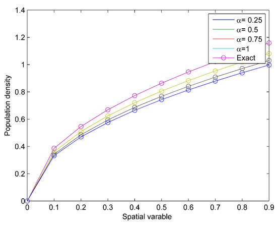
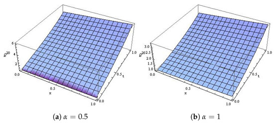
Figure 3 reveals the effect of α and the natural behavior of the model at distinct values of α. Moreover, Figure 4a,b are the surface plots at $\alpha =0.5$ and 1, respectively.

Figure 3. Comparison plot of the exact and approximate solutions for Example 2.

Figure 4. The surface plot for Example 2.

Example 3.

Consider Equation (26) as the time-fractional Fokker–Plane equation [2]:

$${}_0^{ABC}{D}_t^{\beta }Q+{\left(\frac{4}{x}{Q}^2\right)}_x-{\left(\frac{x}{3}Q\right)}_x-{\left(Q^2\right)}_{xx}=0,t>0,0<\beta \le 1,$$

(55)

with the following initial condition.

$$\begin{array}{cc}\hfill & Q_0\left(x\right)=x^2.\hfill \end{array}$$

(56)

From Equations (55) and (56), we set the following.

$$\begin{array}{ccc}& \mathcal{R}\left(Q(x,t)\right)=-{\left(\frac{x}{3}Q\right)}_x,\hfill & \\ & \mathcal{F}\left(Q(x,t)\right)=-{\left(Q^2\right)}_{xx}+{\left(\frac{4}{x}{Q}^2\right)}_x,\hfill & \\ & Q_0(x,0)=x^2.\hfill \end{array}$$

By employing the iteration procedure described in Section 3, we obtain the following.

$$Q_0={\mathcal{A}}^{-1}\left[\frac{1-\beta +\beta {\psi }^{-\beta }}{N\left(\beta \right)}\left(\frac{N\left(\beta \right){\psi }^{-2}\mathcal{Q}(x,0)}{1-\beta +\beta {\psi }^{-\beta }}\right)\right],0<\beta \le 1$$

$$={\mathcal{A}}^{-1}\left[{\psi }^{-2}Q(x,0)\right]$$

(57)

$$={\mathcal{A}}^{-1}\left[{\psi }^{-2}{x}^2\right]$$

$$=x^2,$$

$$Q_1={\mathcal{A}}^{-1}\left[\frac{1-\beta +\beta {\psi }^{-\beta }}{N\left(\beta \right)}\left(\mathcal{A}\left[\mathcal{R}\left(Q_0(x,t)\right)+\mathcal{F}\left(Q_0(x,t)\right)\right]\right)\right]$$

$$={\mathcal{A}}^{-1}\left[\frac{1-\beta +\beta {\psi }^{-\beta }}{N\left(\beta \right)}\left(\mathcal{A}\left[{\left(\frac{x}{3}Q\right)}_x-\left({\left(Q_0^2\right)}_{xx}+{\left(\frac{4}{x}{Q}_0^2\right)}_x\right)\right]\right)\right]$$

(58)

$$={\mathcal{A}}^{-1}\left[\left(\frac{(1-\beta ){\psi }^{\beta }+\beta }{N\left(\beta \right)}\right)\frac{x^2}{{\psi }^{2+\beta }}\right]$$

$$=\left(\frac{(1-\beta ){\psi }^{\beta }+\beta }{N\left(\beta \right)}\right)\frac{x^2{t}^{\beta }}{\mathsf{\Gamma }(\beta +1)},$$

$$Q_2={\mathcal{A}}^{-1}\left[\frac{1-\beta +\beta {\psi }^{-\beta }}{N\left(\beta \right)}\left(\mathcal{A}\left[\mathcal{R}\left(Q_1(x,t)\right)+\left\{\mathcal{F}\left(Q_0(x,t)+Q_1(x,t)\right)-\mathcal{F}\left(Q_0(x,t)\right)\right\}\right]\right)\right]$$

$$\begin{array}{c}\hfill ={\mathcal{A}}^{-1}\left[\frac{1-\beta +\beta {\psi }^{-\beta }}{N\left(\beta \right)}\left(\mathcal{A}\left[\frac{x}{3}{Q}_1+\left\{{\left({(Q_0+Q_1)}^2\right)}_{xx}-{\left(\frac{4}{x}{(Q_0+Q_1)}^2\right)}_x-{\left(Q_0^2\right)}_{xx}+{\left(\frac{4}{x}{Q}_0^2\right)}_x\right\}\right]\right)\right]\\ ={\mathcal{A}}^{-1}\left[{\left(\frac{(1-\beta ){\psi }^{\beta }+\beta }{N\left(\beta \right)}\right)}^2\frac{x^2}{{\psi }^{2+2\beta }}\right]\\ ={\left(\frac{(1-\beta ){\psi }^{\beta }+\beta }{N\left(\beta \right)}\right)}^2\frac{x^2{t}^{2\beta }}{\mathsf{\Gamma }(2\beta +1)},\end{array}$$

(59)

$$⋮$$

$$\begin{array}{c}\hfill Q_k={\mathcal{A}}^{-1}\left[\frac{1-\beta +\beta {\psi }^{-\beta }}{N\left(\beta \right)}\left(\mathcal{A}\left[\mathcal{R}\left(Q_{k-1}(x,t)\right)+\left\{\mathcal{F}\left(\sum _{j=0}^k{Q}_j(x,t)\right)+\mathcal{F}\left(\sum _{j=0}^{k-1}{Q}_j(x,t)\right)\right\}\right]\right)\right]\\ ={\mathcal{A}}^{-1}\left[\frac{1-\beta +\beta {\psi }^{-\beta }}{N\left(\beta \right)}\left(\mathcal{A}\left[{\left(\frac{(1-\beta ){\psi }^{\beta }+\beta }{N\left(\beta \right)}\right)}^{k-1}{Q}_{k-1}(x,t)\right]\right)\right]\\ ={\mathcal{A}}^{-1}\left[{\left(\frac{(1-\beta ){\psi }^{\beta }+\beta }{N\left(\beta \right)}\right)}^k\frac{x^2}{{\psi }^{2+k\beta }}\right]\\ ={\left(\frac{(1-\beta ){\psi }^{\beta }+\beta }{N\left(\beta \right)}\right)}^k\frac{x^2{t}^{k\beta }}{\mathsf{\Gamma }(k\beta +1)},\end{array}$$

(60)

We derived the k-th approximate series solution as the following:

$$\begin{array}{c}{\mathcal{Q}}^{\left(k\right)}(x,t)=\sum _{m=0}^k{Q}_m(x,t)=Q_0(x,0)+Q_1(x,t)+Q_2(x,t)+\cdots +Q_k(x,t)\\ =x^2\left(1+\left(\frac{(1-\beta ){\psi }^{\beta }+\beta }{N\left(\beta \right)}\right)\frac{t^{\beta }}{\mathsf{\Gamma }(\beta +1)}+\cdots +{\left(\frac{(1-\beta ){\psi }^{\beta }+\beta }{N\left(\beta \right)}\right)}^k\frac{t^{k\beta }}{\mathsf{\Gamma }(k\beta +1)}\right)\\ =x^2\sum _{m=0}^k{\left(\frac{(1-\beta ){\psi }^{\beta }+\beta }{N\left(\beta \right)}\right)}^m\frac{t^{m\beta }}{\mathsf{\Gamma }(m\beta +1)},\end{array}$$

(61)

when $k\to \infty$, the k-th order approximate series results in the exact solution.

$$Q(x,t)=\underset{k\to \infty }{lim}{\mathcal{Q}}^{\left(k\right)}(x,t)$$

$$=x^2\underset{k\to \infty }{lim}\sum _{m=0}^k{\left(\frac{(1-\beta ){\psi }^{\beta }+\beta }{N\left(\beta \right)}\right)}^m\frac{t^{m\beta }}{\mathsf{\Gamma }(m\beta +1)}$$

(62)

$$=x^2{E}_{\beta }\left(\frac{((1-\beta ){\psi }^{\beta }+\beta )t^{\beta }}{N\left(\beta \right)}\right),$$

When $\beta =1,$ we obtain the exact solution as follows:

$$=x^2{E}_1\left(t\right)$$

$$=x^2{e}^t,$$

(63)

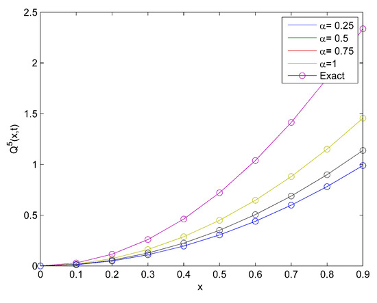
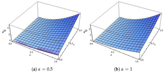
which is the exact solution obtained in [2]. Figure 5 reveals the effect of α and the natural behavior of the model at distinct values of α. Moreover, Figure 6a,b is the surface plot at $\alpha =0.5$ and 1, respectively.

Figure 5. Comparison plot of the exact and approximate solutions for Example 3.

Figure 6. The surface plot for Example 3.

Example 4.

Consider Equation (26) to be the time-fractional Klomogorov equation [2]:

$${}_0^{ABC}{D}_t^{\beta }Q+x^2{e}^t{Q}_{xx}-\left(x+1\right)Q_x=xt,t>0,0<\beta \le 1,$$

(64)

which is subject to the following initial condition.

$$\begin{array}{cc}\hfill & Q_0\left(x\right)=x+1.\hfill \end{array}$$

(65)

From Equations (64) and (65), we set the following.

$$\begin{array}{ccc}& \mathcal{R}\left(Q(x,t)\right)=-x^2{e}^t{Q}_{xx}+\left(x+1\right)Q_x,\hfill & \\ & \mathcal{F}\left(Q(x,t)\right)=0,\hfill & \\ & \mathsf{\Phi }(x,t)=xt,\hfill & \\ & Q_0(x,0)=x+1.\hfill \end{array}$$

By employing the iteration procedure described in Section 3, we obtain the following.

$$Q_0={\mathcal{A}}^{-1}\left[\frac{1-\beta +\beta {\psi }^{-\beta }}{N\left(\beta \right)}\left(\frac{N\left(\beta \right){\psi }^{-2}\mathcal{Q}(x,0)}{1-\beta +\beta {\psi }^{-\beta }}+\mathcal{A}\left[\mathsf{\Phi }(x,t)\right]\right)\right],0<\beta \le 1$$

$$={\mathcal{A}}^{-1}\left[{\psi }^{-2}Q(x,0)+\left(\frac{1-\beta +\beta {\psi }^{-\beta }}{N\left(\beta \right)}\right)\mathcal{A}\left[\mathsf{\Phi }(x,t)\right]\right]$$

(66)

$$={\mathcal{A}}^{-1}\left[{\psi }^{-2}(x+1)+\left(\frac{(1-\beta ){\psi }^{\beta }+\beta }{N\left(\beta \right)}\right)\frac{x}{{\psi }^{3+\beta }}\right]$$

$$=(x+1)+\left(\frac{(1-\beta ){\psi }^{\beta }+\beta }{N\left(\beta \right)}\right)\frac{x{t}^{\beta +1}}{\mathsf{\Gamma }(\beta +2)},$$

$$Q_1={\mathcal{A}}^{-1}\left[\frac{1-\beta +\beta {\psi }^{-\beta }}{N\left(\beta \right)}\left(\mathcal{A}\left[\mathcal{R}\left(Q_0(x,t)\right)+\mathcal{F}\left(Q_0(x,t)\right)\right]\right)\right]$$

$$={\mathcal{A}}^{-1}\left[\frac{1-\beta +\beta {\psi }^{-\beta }}{N\left(\beta \right)}\left(\mathcal{A}\left[-x^2{e}^t{\left(Q_0\right)}_{xx}+\left(x+1\right){\left(Q_0\right)}_x\right]\right)\right]$$

(67)

$$={\mathcal{A}}^{-1}\left[\frac{1-\beta +\beta {\psi }^{-\beta }}{N\left(\beta \right)}\left(\mathcal{A}\left[\left(x+1\right)\left(1+\left(\frac{(1-\beta ){\psi }^{\beta }+\beta }{N\left(\beta \right)}\right)\frac{t^{\beta +1}}{\mathsf{\Gamma }(\beta +2)}\right)\right]\right)\right]$$

$$=(x+1)\left(\left(\frac{(1-\beta ){\psi }^{\beta }+\beta }{N\left(\beta \right)}\right)\frac{t^{\beta }}{\mathsf{\Gamma }(\beta +1)}+{\left(\frac{(1-\beta ){\psi }^{\beta }+\beta }{N\left(\beta \right)}\right)}^2\frac{t^{2\beta +1}}{\mathsf{\Gamma }(2\beta +2)}\right),$$

$$Q_2={\mathcal{A}}^{-1}\left[\frac{1-\beta +\beta {\psi }^{-\beta }}{N\left(\beta \right)}\left(\mathcal{A}\left[\mathcal{R}\left(Q_1(x,t)\right)+\left\{\mathcal{F}\left(Q_0(x,t)+Q_1(x,t)\right)-\mathcal{F}\left(Q_0(x,t)\right)\right\}\right]\right)\right]$$

$$={\mathcal{A}}^{-1}\left[\frac{1-\beta +\beta {\psi }^{-\beta }}{N\left(\beta \right)}\left(\mathcal{A}\left[-x^2{e}^t{\left(Q_1\right)}_{xx}+\left(x+1\right){\left(Q_1\right)}_x\right]\right)\right]$$

(68)

$$={\mathcal{A}}^{-1}\left[\frac{1-\beta +\beta {\psi }^{-\beta }}{N\left(\beta \right)}\left(\mathcal{A}\left[(x+1)\left(\frac{1-\beta +\beta {\psi }^{-\beta }}{N\left(\beta \right)}\right)\frac{t^{\beta }}{\mathsf{\Gamma }(\beta +1)}+{\left(\frac{1-\beta +\beta {\psi }^{-\beta }}{N\left(\beta \right)}\right)}^2\frac{t^{2\beta +1}}{\mathsf{\Gamma }(2\beta +2)}\right]\right)\right]$$

$$=(x+1)\left({\left(\frac{(1-\beta ){\psi }^{\beta }+\beta }{N\left(\beta \right)}\right)}^2\frac{t^{2\beta }}{\mathsf{\Gamma }(2\beta +1)}+{\left(\frac{(1-\beta ){\psi }^{\beta }+\beta }{N\left(\beta \right)}\right)}^3\frac{t^{3\beta +1}}{\mathsf{\Gamma }(3\beta +2)}\right),$$

$$⋮$$

$$\begin{array}{c}\hfill Q_k={\mathcal{A}}^{-1}\left[\frac{1-\beta +\beta {\psi }^{-\beta }}{N\left(\beta \right)}\left(\mathcal{A}\left[\mathcal{R}\left(Q_{k-1}(x,t)\right)+\left\{\mathcal{F}\left(\sum _{j=0}^k{Q}_j(x,t)\right)+\mathcal{F}\left(\sum _{j=0}^{k-1}{Q}_j(x,t)\right)\right\}\right]\right)\right]\end{array}$$

$$={\mathcal{A}}^{-1}\left[\frac{1-\beta +\beta {\psi }^{-\beta }}{N\left(\beta \right)}\left(\mathcal{A}\left[{\left(\frac{(1-\beta ){\psi }^{\beta }+\beta }{N\left(\beta \right)}\right)}^{k-1}{\left(Q_{k-1}(x,t)\right)}_x\right]\right)\right]$$

(69)

$$={\mathcal{A}}^{-1}\left[(x+1)\left(\frac{1}{{\psi }^{2+k\beta }}{\left(\frac{(1-\beta ){\psi }^{\beta }+\beta }{N\left(\beta \right)}\right)}^k+\frac{1}{{\psi }^{3+(k+1)\beta }}{\left(\frac{(1-\beta ){\psi }^{\beta }+\beta }{N\left(\beta \right)}\right)}^{k+1}\right)\right]$$

$$=(x+1)\left({\left(\frac{(1-\beta ){\psi }^{\beta }+\beta }{N\left(\beta \right)}\right)}^k\frac{t^{k\beta }}{\mathsf{\Gamma }(k\beta +1)}+{\left(\frac{(1-\beta ){\psi }^{\beta }+\beta }{N\left(\beta \right)}\right)}^{k+1}\frac{t^{(k+1)\beta +1}}{\mathsf{\Gamma }\left(\right(k+1)\beta +2)}\right),$$

We derived the k-th approximate series solution as the following.

$$\begin{array}{c}{\mathcal{Q}}^{\left(k\right)}(x,t)=\sum _{m=0}^k{Q}_m(x,t)=Q_0(x,0)+Q_1(x,t)+Q_2(x,t)+\cdots +Q_k(x,t)\\ =(x+1)+\left((x+1)-1\right)\frac{t^{\beta +1}}{\mathsf{\Gamma }(\beta +2)}\left(\frac{(1-\beta ){\psi }^{\beta }+\beta }{N\left(\beta \right)}\right)+\\ (x+1)\left(\left(\frac{(1-\beta ){\psi }^{\beta }+\beta }{N\left(\beta \right)}\right)\frac{t^{\beta }}{\mathsf{\Gamma }(\beta +1)}+{\left(\frac{(1-\beta ){\psi }^{\beta }+\beta }{N\left(\beta \right)}\right)}^2\frac{t^{2\beta +1}}{\mathsf{\Gamma }(2\beta +2)}\right)+\\ (x+1)\left({\left(\frac{(1-\beta ){\psi }^{\beta }+\beta }{N\left(\beta \right)}\right)}^2\frac{t^{2\beta }}{\mathsf{\Gamma }(2\beta +1)}+{\left(\frac{(1-\beta ){\psi }^{\beta }+\beta }{N\left(\beta \right)}\right)}^3\frac{t^{3\beta +1}}{\mathsf{\Gamma }(3\beta +2)}\right)+\\ \hfill \cdots +(x+1)\left({\left(\frac{(1-\beta ){\psi }^{\beta }+\beta }{N\left(\beta \right)}\right)}^k\frac{t^{k\beta }}{\mathsf{\Gamma }(k\beta +1)}+{\left(\frac{(1-\beta ){\psi }^{\beta }+\beta }{N\left(\beta \right)}\right)}^{(k+1)}\frac{t^{(k+1)\beta +1}}{\mathsf{\Gamma }\left(\right(k+1)\beta +2)}\right),\end{array}$$

(70)

when $k\to \infty$, the k-th order approximate series results in the exact solution:

$$\begin{array}{c}Q(x,t)=\underset{k\to \infty }{lim}{\mathcal{Q}}^{\left(k\right)}(x,t)\\ =\frac{-t^{\beta +1}}{\mathsf{\Gamma }(\beta +2)}\left(\frac{(1-\beta ){\psi }^{\beta }+\beta }{N\left(\beta \right)}\right)+(x+1)\left(E_{\beta }\left(\frac{(1-\beta ){\psi }^{\beta }+\beta }{N\left(\beta \right)}\right)\right)+\\ \hfill (x+1)\underset{k\to \infty }{lim}\sum _{m=0}^k{\left(\frac{(1-\beta ){\psi }^{\beta }+\beta }{N\left(\beta \right)}\right)}^{m+1}\frac{t^{(m+1)\beta +1}}{\mathsf{\Gamma }\left(\right(m+1)\beta +2)},\end{array}$$

(71)

When $\beta =1,$ we obtain the exact solution as follows:

$$=\frac{-t^2}{2}+(x+1)\left(E_1\left(t\right)+\underset{k\to \infty }{lim}\sum _{m=0}^k\frac{t^{m+2}}{\mathsf{\Gamma }(m+3)}\right)$$

$$=\frac{-t^2}{2}+(x+1)\left(2e^t-t-1\right),$$

(72)

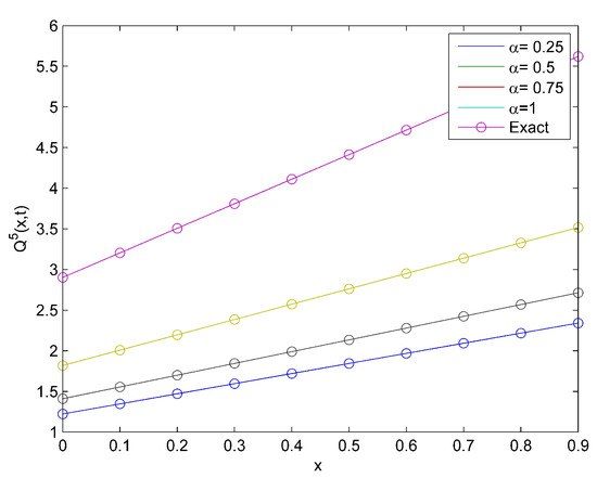
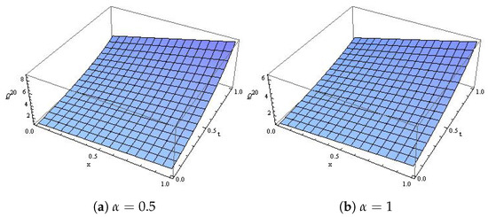
which is the exact solution obtained [2]. Figure 7 reveals the effect of α and the natural behavior of the model at distinct values of α. Moreover, Figure 8a,b is the surface plot at $\alpha =0.5$ and 1, respectively.

Figure 7. Comparison plot of the exact and approximate solutions for Example 4.

Figure 8. The surface plot for Example 4.

Example 5.

Consider Equation (26) as the one dimensional time-fractional biological population model according to Verhulst law [26]:

$${}_0^{ABC}{D}_t^{\beta }Q={\left(Q^2\right)}_{xx}+\frac{1}{4}Q,t>0,0<\beta \le 1,$$

(73)

that is subject to the following initial condition.

$$\begin{array}{cc}\hfill & Q_0\left(x\right)=x^{\frac{1}{2}}.\hfill \end{array}$$

(74)

From Equations (73) and (74), we set the following.

$$\begin{array}{ccc}& \mathcal{R}\left(Q(x,t)\right)=\frac{1}{4}Q,\hfill & \\ & \mathcal{F}\left(Q(x,t)\right)={\left(Q^2\right)}_{xx},\hfill & \\ & Q_0(x,0)=x^{\frac{1}{2}}.\hfill \end{array}$$

By employing the iteration procedure described in Section 3, we obtain the following.

$$Q_0={\mathcal{A}}^{-1}\left[\frac{1-\beta +\beta {\psi }^{-\beta }}{N\left(\beta \right)}\left(\frac{N\left(\beta \right){\psi }^{-2}\mathcal{Q}(x,0)}{1-\beta +\beta {\psi }^{-\beta }}\right)\right],0<\beta \le 1$$

$$={\mathcal{A}}^{-1}\left[{\psi }^{-2}Q(x,0)\right]$$

(75)

$$={\mathcal{A}}^{-1}\left[{\psi }^{-2}{x}^{\frac{1}{2}}\right]$$

$$=x^{\frac{1}{2}}.$$

$$Q_1={\mathcal{A}}^{-1}\left[\frac{1-\beta +\beta {\psi }^{-\beta }}{N\left(\beta \right)}\left(\mathcal{A}\left[\mathcal{R}\left(Q_0(x,t)\right)+\mathcal{F}\left(Q_0(x,t)\right)\right]\right)\right]$$

$$={\mathcal{A}}^{-1}\left[\frac{1-\beta +\beta {\psi }^{-\beta }}{N\left(\beta \right)}\left(\mathcal{A}\left[\frac{1}{4}{Q}_0+{\left(Q_0^2\right)}_{xx}\right]\right)\right]$$

$$={\mathcal{A}}^{-1}\left[\left(\frac{(1-\beta ){\psi }^{\beta }+\beta }{N\left(\beta \right)}\right)\frac{\left(\frac{1}{4}\right)}{{\psi }^{2+\beta }}{x}^{\frac{1}{2}}\right]$$

(76)

$$=\left(\frac{(1-\beta ){\psi }^{\beta }+\beta }{N\left(\beta \right)}\right)\frac{\left(\frac{1}{4}\right)t^{\beta }}{\mathsf{\Gamma }(\beta +1)}{x}^{\frac{1}{2}},$$

$$Q_2={\mathcal{A}}^{-1}\left[\frac{1-\beta +\beta {\psi }^{-\beta }}{N\left(\beta \right)}\left(\mathcal{A}\left[\mathcal{R}\left(Q_1(x,t)\right)+\left\{\mathcal{F}\left(Q_0(x,t)+Q_1(x,t)\right)-\mathcal{F}\left(Q_0(x,t)\right)\right\}\right]\right)\right]$$

$$={\mathcal{A}}^{-1}\left[\frac{1-\beta +\beta {\psi }^{-\beta }}{N\left(\beta \right)}\left(\mathcal{A}\left[\frac{1}{4}{Q}_1+\left\{{\left({\left(Q_0+Q_1\right)}^2\right)}_{xx}\right\}\right]\right)\right]$$

$$={\mathcal{A}}^{-1}\left[{\left(\frac{(1-\beta ){\psi }^{\beta }+\beta }{N\left(\beta \right)}\right)}^2\frac{{\left(\frac{1}{4}\right)}^2}{{\psi }^{2+2\beta }}{x}^{\frac{1}{2}}\right]$$

(77)

$$={\left(\frac{(1-\beta ){\psi }^{\beta }+\beta }{N\left(\beta \right)}\right)}^2\frac{{\left(\frac{1}{4}{t}^{\beta }\right)}^2}{\mathsf{\Gamma }(2\beta +1)}{x}^{\frac{1}{2}},$$

$$⋮$$

$$\begin{array}{c}\hfill Q_k={\mathcal{A}}^{-1}\left[\frac{1-\beta +\beta {\psi }^{-\beta }}{N\left(\beta \right)}\left(\mathcal{A}\left[\mathcal{R}\left(Q_{k-1}(x,t)\right)+\left\{\mathcal{F}\left(\sum _{j=0}^k{Q}_j(x,t)\right)+\mathcal{F}\left(\sum _{j=0}^{k-1}{Q}_j(x,t)\right)\right\}\right]\right)\right]\end{array}$$

$$={\mathcal{A}}^{-1}\left[\frac{1-\beta +\beta {\psi }^{-\beta }}{N\left(\beta \right)}\left(\mathcal{A}\left[{\left(\frac{(1-\beta ){\psi }^{\beta }+\beta }{N\left(\beta \right)}\right)}^{k-1}\frac{1}{4}{Q}_{k-1}(x,t)\right]\right)\right]$$

(78)

$$={\mathcal{A}}^{-1}\left[{\left(\frac{(1-\beta ){\psi }^{\beta }+\beta }{N\left(\beta \right)}\right)}^k\frac{e^{\frac{1}{5}x}}{{\psi }^{2+k\beta }}\right]$$

$$={\left(\frac{(1-\beta ){\psi }^{\beta }+\beta }{N\left(\beta \right)}\right)}^k\frac{{\left(\frac{1}{4}{t}^{\beta }\right)}^k}{\mathsf{\Gamma }(k\beta +1)}{x}^{\frac{1}{2}},$$

We derived the k-th approximate series solution as the following.

$${\mathcal{Q}}^{\left(k\right)}(x,t)=\sum _{m=0}^k{Q}_m(x,t)=Q_0(x,0)+Q_1(x,t)+Q_2(x,t)+\cdots +Q_k(x,t)$$

$$=x^{\frac{1}{2}}\left(1+\left(\frac{(1-\beta ){\psi }^{\beta }+\beta }{N\left(\beta \right)}\right)\frac{\frac{1}{4}{t}^{\beta }}{\mathsf{\Gamma }(\beta +1)}+\cdots +{\left(\frac{(1-\beta ){\psi }^{\beta }+\beta }{N\left(\beta \right)}\right)}^k\frac{{\left(\frac{1}{4}{t}^{\beta }\right)}^k}{\mathsf{\Gamma }(k\beta +1)}\right)$$

$$=x^{\frac{1}{2}}\sum _{m=0}^k{\left(\frac{(1-\beta ){\psi }^{\beta }+\beta }{N\left(\beta \right)}\right)}^m\frac{{\left(\frac{1}{4}{t}^{\beta }\right)}^m}{\mathsf{\Gamma }(m\beta +1)},$$

(79)

when $k\to \infty$, the k-th order approximate series results in the exact solution.

$$Q(x,t)=\underset{k\to \infty }{lim}{\mathcal{Q}}^{\left(k\right)}(x,t)$$

$$=x^{\frac{1}{2}}\underset{k\to \infty }{lim}\sum _{m=0}^k{\left(\frac{(1-\beta ){\psi }^{\beta }+\beta }{N\left(\beta \right)}\right)}^m\frac{{\left(\frac{1}{4}{t}^{\beta }\right)}^m}{\mathsf{\Gamma }(m\beta +1)}$$

(80)

$$=x^{\frac{1}{2}}{E}_{\beta }\left(\frac{((1-\beta ){\psi }^{\beta }+\beta )\frac{1}{4}{t}^{\beta }}{N\left(\beta \right)}\right),$$

When $\beta =1,$ we obtain the exact solution as the following:

$$=x^{\frac{1}{2}}{E}_1\left(\frac{1}{4}t\right)$$

$$=x^{\left(\frac{1}{2}\right)}{e}^{\frac{t}{4}},$$

(81)

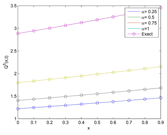
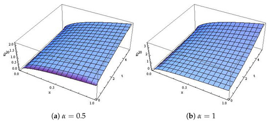
which is the exact solution obtained in [4]. Figure 9 reveals the effect of α and the natural behavior of the model at distinct values of α. Moreover, Figure 10a,b is the surface plot at $\alpha =0.5$ and 1, respectively.

Figure 9. Comparison plot of the exact and approximate for Example 5.

Figure 10. The surface plot for Example 5.

5. Conclusions

In this paper, we utilized the connection between the Aboodh transform and the Laplace transform to establish the Aboodh transform of Atangana–Baleanu fractional differential operator. The accuracy and validity of the Aboodh transform iterative method for fractional differential equation with Atangana–Baleanu fractional differential operator are also presented.

The graphical illustration in Figure 1, Figure 2, Figure 3, Figure 4, Figure 5, Figure 6, Figure 7, Figure 8, Figure 9 and Figure 10 is presented to validate the effectiveness of the Aboodh transform iterative method and to capture the natural behavior of differential equation with the Atangana–Baleanu fractional differential operator.

Finally, we conclude that Atangana–Baleanu fractional differential operator contains a local and a singular kernel that makes the Atangana–Baleanu fractional differential operator more suitable for real life applications and that the Aboodh transform iterative method can adequately capture the effect and the behavior of fractional differential equations.

References

- Iyiola, O.S.; Ojo, G.O. On the analytical solution of Fornberg–Whitham equation with the new fractional derivative. Pramana 2015, 85, 567–575. [Google Scholar] [CrossRef]
- Akinyemi, L.; Iyiola, O.S. Exact and approximate solutions of time-fractional models arising from physics via Shehu transform. Math. Methods Appl. Sci. 2020, 43, 7442–7464. [Google Scholar] [CrossRef]
- Iyiola, O.S.; Ojo, G.O.; Mmaduabuchi, O. The fractional Rosenau–Hyman model and its approximate solution. Alex. Eng. J. 2016, 55, 1655–1659. [Google Scholar] [CrossRef] [Green Version]
- Ojo, G.O.; Mahmudov, N.I. Aboodh Transform Iterative Method for Spatial Diffusion of a Biological Population with Fractional-Order. Mathematics 2021, 9, 155. [Google Scholar] [CrossRef]
- Iyiola, O.S.; Ojo, G.O.; Audu, J.D. A Comparison Results of Some Analytical Solutions of Model in Double Phase Flow through Porous Media. J. Math. Syst. Sci. 2014, 4, 275–284. [Google Scholar]
- Podlubny, I. Fractional Differential Equations: An Introduction to Fractional Derivatives, Fractional Differential Equations, to Methods of Their Solution and Some of Their Applications; Elsevier: Amsterdam, The Netherlands, 1998. [Google Scholar]
- Oldham, K.; Spanier, J. The Fractional Calculus Theory and Applications of Differentiation and Integration to Arbitrary Order; Academic Press: New York, NY, USA, 1974. [Google Scholar]
- Miller, K.S.; Ross, B. An Introduction to the Fractional Calculus and Fractional Differential Equations; Wiley: New York, NY, USA, 1993. [Google Scholar]
- Kilbas, A.A.; Srivastava, H.M.; Trujillo, J.J. Theory and Applications of Fractional Differential Equations; Elsevier: Amsterdam, The Netherlands, 2006; Volume 204. [Google Scholar]
- Diethelm, K. The Analysis of Fractional Differential Equations: An Application-Oriented Exposition Using Differential Operators of Caputo Type; Springer Science and Business Media: Heidelberg, Germany, 2010. [Google Scholar]
- Atangana, A.; Baleanu, D. New fractional derivatives with nonlocal and non-singular kernel: Theory and application to heat transfer model. Therm. Sci. 2016, 20, 763–769. [Google Scholar] [CrossRef] [Green Version]
- Caputo, M.; Fabrizio, M. A new definition of fractional derivative without singular kernel. Progr. Fract. Differ. Appl. 2015, 1, 1–13. [Google Scholar]
- Gondal, M.A.; Arife, A.S.; Khan, M.; Hussain, I. An efficient numerical method for solving linear and nonlinear partial differential equations by combining homotopy analysis and transform method. World Appl. Sci. J. 2011, 15, 1786–1791. [Google Scholar]
- Arafa, A.A.; Hagag, A.M.S. Q-homotopy analysis transform method applied to fractional Kundu–Eckhaus equation and fractional massive Thirring model arising in quantum field theory. Asian-Eur. J. Math. 2019, 12, 1950045. [Google Scholar] [CrossRef]
- Arafa, A.A.; Hagag, A.M.S. A new analytic solution of fractional coupled Ramani equation. Chin. J. Phys. 2019, 60, 388–406. [Google Scholar] [CrossRef]
- Saad, K.M.; AL-Shareef, E.H.; Alomari, A.K.; Baleanu, D.; Gómez-Aguilar, J.F. On exact solutions for time-fractional Korteweg-de Vries and Korteweg-de Vries-Burger’s equations using homotopy analysis transform method. Chin. J. Phys. 2020, 63, 149–162. [Google Scholar] [CrossRef]
- Enyi, C.D. Efficacious Analytical Technique Applied to Fractional Fornberg–Whitham Model and Two-Dimensional Fractional Population Model. Symmetry 2020, 12, 1976. [Google Scholar] [CrossRef]
- Baleanu, D.; Mohammadi, H.; Rezapour, S. Analysis of the model of HIV-1 infection of CD4+ T-cell with a new approach of fractional derivative. Adv. Differ. Equ. 2020, 71, 1–17. [Google Scholar] [CrossRef] [Green Version]
- Aydogan, M.S.; Baleanu, D.; Mousalou, A.; Rezapour, S. On high order fractional integro-differential equations including the Caputo–Fabrizio derivative. Bound. Value Probl. 2018, 2018, 90. [Google Scholar] [CrossRef]
- Atangana, A.; Koca, I. Chaos in a simple nonlinear system with Atangana–Baleanu derivatives with fractional order. Chaos Solitons Fractals 2016, 89, 447–454. [Google Scholar] [CrossRef]
- Bokhari, A.; Baleanu, D.; Belgacem, R. Application of Shehu transform to Atangana-Baleanu derivatives. J. Math. Comput. Sci. 2020, 20, 101–107. [Google Scholar] [CrossRef] [Green Version]
- Debnath, I.; Bhatta, D. Integral Transforms and Their Application; CRC Press: Boca Raton, FL, USA, 2014. [Google Scholar]
- Aboodh, K.S.; Idris, A.; Nuruddeen, R.I. On the Aboodh transform connections with some famous integral transforms. Int. J. Eng. Inform. Syst. 2017, 1, 143–151. [Google Scholar]
- Mittag-Leffler, M.G. Sur La nonvelle Fonction Eα(x). Comptes Rendus Acad. Sci. Paris 1903, 2, 1003. [Google Scholar]
- Daftardar-Gejji, V.; Jafari, H. An iterative method for solving nonlinear functional equations. J. Math. Anal. Appl. 2006, 316, 753–763. [Google Scholar] [CrossRef] [Green Version]
- Gurtin, M.E.; MacCamy, R.C. On the diffusion of biological populations. Math. Biosci. 1977, 33, 35–49. [Google Scholar] [CrossRef]
Publisher’s Note: MDPI stays neutral with regard to jurisdictional claims in published maps and institutional affiliations. |
© 2021 by the authors. Licensee MDPI, Basel, Switzerland. This article is an open access article distributed under the terms and conditions of the Creative Commons Attribution (CC BY) license (https://creativecommons.org/licenses/by/4.0/).