λ-Interval of Triple Positive Solutions for the Perturbed Gelfand Problem

Abstract

We study a two-point Boundary Value Problem depending on two parameters that represents a mathematical model arising from the combustion theory. Applying fixed point theorems for concave operators, we prove uniqueness, existence, upper, and lower bounds of positive solutions. In addition, we give an estimation for the value of ${\lambda }_{*}$ such that, for the parameter $\lambda \in [{\lambda }_{*},{\lambda }^{*}]$, there exist exactly three positive solutions. Numerical examples are presented to illustrate various cases. The results complement previous work on this problem.

1. Introduction

As a mathematical model arising from the combustion theory [1,2], the following two-point Boundary Value Problem (BVP) has been well studied by a number of authors [3,4,5,6,7,8,9,10]:

$$\{\begin{array}{c}{u}^{″}\left(t\right)+\lambda exp\left(\frac{\alpha u\left(t\right)}{\alpha +u\left(t\right)}\right)=0,-1<t<1,\hfill \\ u(-1)=u\left(1\right)=0,\hfill \end{array}$$

(1)

where $\lambda >0$ is the Frank–Kamenetskii parameter, $\alpha >0$ is the activation energy parameter, u is the dimensionless temperature, and the reaction term $exp\left(\frac{\alpha u}{\alpha +u}\right)$ shows the temperature dependence. Representing the steady case in the thermal explosion, BVP (1.1) is well-known as the one-dimensional perturbed Gelfand problem [1,2,5].

In the literature, bifurcation curve, existence, and multiplicity of positive solutions for BVP (1.1) have been extensively studied. In particular, Shivaji [8] first shows that, for every $\alpha >0$, BVP (1.1) has a unique nonnegative solution when $\lambda$ is small enough or large enough. Hastings and McLeod [4] and Brown et al. [3] prove that the bifurcation curve of (1.1) is S-shaped on the $(\lambda ,$$\parallel u\parallel )$ plane when $\alpha$ is large enough, where $\parallel u\parallel$ is the norm in the space $C[-1,1]$. That is, when $\alpha$ is large enough, there exist ${\lambda }_{*}$, ${\lambda }^{*}$ such that (1.1) has a unique nonnegative solution for $0<\lambda <{\lambda }_{*}$, $\lambda >{\lambda }^{*}$, exactly three nonnegative solutions for ${\lambda }_{*}<\lambda <{\lambda }^{*}$, and exactly two nonnegative solutions for $\lambda ={\lambda }_{*}\left(\alpha \right)$ and ${\lambda }^{*}\left(\alpha \right)$. Later, it was proved that the BVP (1.1) has multiple solutions when $\alpha >4.4967$ [11]. This lower bound was improved to 4.35 by Korman and Li [12]. Recently, it was shown in [5,6] that the number can be as close to 4 as 4.166. The problem has also been considered for general operator equations in abstract Banach spaces [10]. Most recently, a similar problem has been studied for the Neumann boundary value problem [9]. The techniques applied mostly are the quadrature method.

In this paper, we first apply a new result on a unique solution for a class of concave operators in a partially ordered Banach space [13] to prove that there exists a unique solution for BVP (1.1) when $\alpha \le 4$. Previously, it was shown that, when $\alpha \le 4$, the bifurcation curve for $(\lambda ,$$\parallel u\parallel )$ is monotonically increasing, which implies that the sup norm of the solutions must be unique [11]. With a totally different approach, we are able to directly prove the uniqueness of solutions. Then, we prove a general result for all parameters on the existence of a solution using a new fixed point theorem on order intervals that was recently introduced in [14]. As an advantage of this new method, we obtain upper and lower bounds of the solutions depending on the values of $\lambda$ and $\alpha$. Next, assuming that $\alpha >4$, it is known that there exists an $\lambda$-interval (${\lambda }_{*},{\lambda }^{*})$ such that BVP (1.1) has at least three nonnegative solutions for $\lambda \in ({\lambda }_{*},{\lambda }^{*})$ [3,4,5,6,11,12]. However, nothing is known for the range of the $\lambda$-interval, or the values of ${\lambda }_{*}$ and ${\lambda }^{*}$. We obtain a range of ${\lambda }_{*}$ by an upper bound and a lower bound. The accuracy of the estimation is shown by the fact that the range is usually very small. From our knowledge, this is the first time to give a concrete estimation for the $\lambda$-intervals that ensure solution multiplicity. Lastly, some numerical results are given to illustrate the upper and lower bounds and multiplicity of solutions.

The rest of the paper is organized as the following: Section 2 provides some preliminary results that will be used in the sequel. Section 3 proves the uniqueness theorem. Section 4 discusses existence, upper, and lower bounds of solutions. Section 5 gives the $\lambda$-intervals for multiplicity. Numerical solutions obtained by MatLab are presented in Section 6.

2. Preliminary

Let ($E,\parallel .\parallel )$ be a real Banach space and $\theta$ be the zero element of E. We first introduce the concept of order cone.

Definition 1

([15], p. 276). A subset P of E is called an order cone iff:

(i)

P is closed, nonempty, and $P\ne \left\{0\right\}$;

(ii)

$a,b\in \mathbb{R},a,b\ge 0,x,y\in P\Rightarrow ax+by\in P$;

(iii)

$x\in P$ and $-x\in P\Rightarrow x=0.$

A Banach space E is partially ordered by an order cone P, i.e., $x\le y$ if and only if $y-x\in P$ for any $x,y\in E.$ P is normal if there exists $N>0$ such that $\parallel x\parallel \le N\parallel y\parallel$ if $x,y\in E$ and $\theta \le x\le y.$ The infimum of such constants N is called the normality constant of P. Following the notation of [13,16], for $x,y\in E$, $x\sim y$ means that there exist $\lambda >0$ and $\mu >0$ such that $\lambda x\le y\le \mu x.$ It is clear that ∼ is an equivalence relation. For fixed $h>\theta ,$$P_h=\{x\in E|x\sim h\}.$ It is easy to see that $P_h\subset P$.

Definition 2.

An operator $A:E\to E$ is increasing if $x\le y$ implies $Ax\le Ay.$

Definition 3

([13]). Let $e\in P$ with $\theta \le e\le h.$ Define the set

$$P_{h,e}=\{x\in E|x+e\in P_h\}.$$

An operator $A:P_{h,e}\to E$ is said to be a ϕ-$(h,e)$-concave operator if there exists $\varphi \left(\lambda \right)>\lambda$ for $\lambda \in (0,1)$ such that

$$A(\lambda x+(\lambda -1)e)\ge \varphi \left(\lambda \right)Ax+(\varphi \left(\lambda \right)-1)e for any x\in P_{h,e}.$$

Theorem 1

([16]). Suppose that A is an increasing ϕ-$(h,\theta )$-concave operator, P is normal, and $Ah\in P_h.$ Then, A has a unique fixed point $x^{*}$ in $P_h.$ Moreover, for any given point $w_0\in P_h,$$\parallel w_n-x^{*}\parallel \to 0$ as $n\to \infty$ if $w_n=A{w}_{n-1}$ for $n=1,2,\dots$.

Theorem 2

([14]). Assume that X is an ordered Banach space with the order cone $X_{+}.$ Let $0\le u_0\le \varphi$ be such that $\parallel u_0\parallel \le 1$ and $\parallel \varphi \parallel =1$ satisfying the condition that if $x\in X_{+},\parallel x\parallel \le 1,$ then $x\le \varphi$. If there exist positive numbers, $0<a<b$ such that $T:$$P_{u_0}\bigcap (\overline{{\mathsf{\Omega }}_b}\backslash {\mathsf{\Omega }}_a)\to P_{u_0}$ is a completely continuous operator. If the conditions

$${\left|\right|T\left(x\right)\left|\right|}_{x\in [a{u}_0,a\varphi ]}\le {a, and \parallel T\left(x\right)\parallel }_{x\in [b{u}_0,b\varphi ]}\ge b$$

(2)

or

$${\parallel T\left(x\right)\parallel }_{x\in [a{u}_0,a\varphi ]}\ge {a, and \parallel T\left(x\right)\parallel }_{x\in [b{u}_0,b\varphi ]}\le b$$

(3)

are satisfied, then T has a fixed point $x_0\in [a{u}_0,$$b\varphi ].$

3. Uniqueness for $\mathit{\alpha }\le \mathbf{4}$

In this section, we apply Theorem 1 to prove the following theorem on existence and uniqueness of solutions for BVP (1.1) with the assumption of $\alpha \le 4$.

Let $X=C[-1,1]$ with the standard norm $u\in X$, $\parallel u\parallel ={max}_{-1\le t\le 1}\left|u\left(t\right)\right|$. Let $P=\left\{u\right|u\in X,u\left(t\right)\ge 0,t\in [-1,1]\}$. It is clear that P is a normal cone of $C[-1,1]$.

Theorem 3.

BVP problem (1.1) has a unique solution for all $\alpha \le 4.$

Proof. 

It can be verified that $u\in X$ is a solution of BVP (1.1) if and only if $Tu=u$, where $T:X\to X$ is the Hammerstein integral operator defined as

$$\left(Tu\right)\left(t\right)=\frac{\lambda }{2}{\int }_{-1}^{1}G(s,t)exp\left(\frac{\alpha u\left(s\right)}{\alpha +u\left(s\right)}\right)ds,t\in [-1,1],$$

(4)

and the Green’s function $G(s,t)$ is calculated as

$$G(s,t)=\{\begin{array}{c}(1-t)(1+s),-1<s\le t<1,\\ (1+t)(1-s),-1<t\le s<1.\end{array}$$

It is easy to see that $(1-|s\left|\right)(1-|t\left|\right)<G(s,t)\le 1-s^2$ for all $-1<s<1$ and $-1<t<1$ and ${\int }_{-1}^{1}G(s,t)ds=1-t^2$.

Since both $\lambda$ and G are positive and the function $f\left(x\right)=exp\left(\frac{ax}{a+x}\right)$ is increasing with respect to $x,$ the operator T is increasing. Let $h\left(t\right)=1-t^2$. One can easily find that

$$\frac{\lambda }{2}(1-t^2)\le Tu\left(t\right)\le \frac{\lambda }{2}{e}^{\alpha }(1-t^2).$$

Therefore, $Th\left(t\right)\in P_{h,\theta }$, where $P_{h,\theta }$ is defined by Definition 3.

To prove that $T:$$P_{h,\theta }\to X$ is a $\varphi$-$(h,\theta )$-concave operator, denote $f\left(x\right)=exp\left(\frac{x}{1+ϵx}\right)$ for $ϵ=\frac{1}{a}$ and let $\varphi \left(\mu \right)=\frac{f\left(\mu x\right)}{f\left(x\right)}=exp(\frac{\mu x}{1+ϵ\mu x}-\frac{x}{1+ϵx})$. Then,

$${\varphi }^{\prime }\left(\mu \right)\left(x\right)=\varphi \left(\mu \right)\left(x\right)\frac{\mu {(1+ϵx)}^2-{(1+ϵ\mu x)}^2}{{(1+ϵx)}^2{(1+ϵ\mu x)}^2}.$$

Since $\varphi \left(\mu \right)>0$, the numerator is the only part that may change sign. It can be verified that the numerator is less than 0 when $x\in [0,\frac{1}{ϵ\sqrt{\mu }}]$ and greater than 0 when $x\in [\frac{1}{ϵ\sqrt{\mu }},\infty ].$ Therefore, $\varphi \left(\mu \right)$ has only one critical point at $x=\frac{1}{ϵ\sqrt{\mu }}$ and it has its minimum value $\varphi \left(\mu \right)\left(\frac{1}{ϵ\sqrt{\mu }}\right)=exp\left(\frac{\sqrt{\mu }-1}{(\sqrt{\mu }+1)ϵ}\right)$. Hence, $f\left(\mu x\right)\ge \varphi \left(\mu \right)f\left(x\right)$.

Next, denoting $k\left(\mu \right)=\frac{\sqrt{\mu }-1}{(\sqrt{\mu }+1)ln\mu }<ϵ$, we show that $k^{\prime }\left(\mu \right)>0$. Let $q\left(\mu \right)=ln\mu -{\mu }^{\frac{1}{2}}+{\mu }^{-\frac{1}{2}}$. Then, $q^{\prime }\left(\mu \right)=-\frac{1}{2}{\mu }^{-\frac{3}{2}}{(\sqrt{\mu }-1)}^2<0$, $q\left(1\right)=0$ and $q\left(\mu \right)>0$ ensure that $k^{\prime }\left(\mu \right)>0$ for all $\mu \in (0,1).$ It follows that k is increasing and its superum over $(0,1)$ is $\frac{1}{4}$. Hence, the inequality $ϵ\ge \frac{1}{4}$ or $\alpha \le 4$ implies that $\varphi \left(\mu \right)>\mu$ with all $\mu \in (0,1).$ Consequently, the operator T defined (3.1) satisfies all the conditions of Theorem 1 when $\alpha \le 4$, and it has a unique fixed point in $P_{h,\theta }$. Since operator (3.1) guarantees that all solutions are in $P_h$, BVP (1.1) has a unique solution when $\alpha \le 4$ for every $\lambda >0$. □

Remark 1.

Existence of solutions for BVP (1.1) was previously shown by the S-shaped bifurcation curve on $(\lambda ,\parallel u\parallel )$ [3,4,6,11]. Since the bifurcation curve depends on $\parallel u\parallel$, some qualitative properties for the maximum of solutions can be observed. For example, it was proved in [3] that the sup norm of the solutions of BVP (1.1) is unique when $\alpha \le 4$.

4. Upper, Lower Bounds and Order Sequence of Solutions

In this section, we prove the existence of upper and lower bounds for the general case of BVP (1.1). The approach is by Theorem 2, a new fixed point theorem on order intervals recently introduced in [14].

Let $X,P$ and f be defined as in the proof of Theorem 3 and $g\left(x\right)=\frac{f\left(x\right)}{x}$. Then, g has the properties of

$$\underset{x\to 0^{+}}{lim}g\left(x\right)=\infty ,\hspace{1em}\underset{x\to \infty }{lim}g\left(x\right)\to 0.$$

(5)

Theorem 4.

Select positive parameters $a,b$, and δ such that

$$a=\frac{\lambda }{2},g\left(b\right)=\frac{2}{\lambda },\delta =\frac{\lambda }{2b}.$$

(6)

Then BVP (1.1) has a solution u such that

$$\frac{\lambda }{2}\delta (1-t^2)\le \delta u\left(0\right)(1-t^2)\le u\left(t\right)\le b(1-t^2),t\in [0,1].$$

(7)

Proof. 

From the proof of Theorem 3, $u\in X$ is a solution of BVP (1.1) if and only if $Tu=u$, where T is defined by (4). Let $u_0=\delta (1-t^2)$ and $\phi =1$. Then, $u_0$ and $\phi$ satisfy the conditions of Theorem 2. Define

$$P_{u_0}=\{u\in P|\parallel u\parallel =u\left(0\right),u(-t)=u\left(t\right),u\left(t\right)\ge \delta u\left(0\right)(1-t^2),t\in [-1,1]\}.$$

It can be verified that $P_{u_0}$ is a subcone of P. To prove $T:P_{u_0}\cap (\overline{{\mathsf{\Omega }}_b}\backslash {\mathsf{\Omega }}_a)\to P_{u_0}$, let $u\in P_{u_0}$ with $\parallel u\parallel \le b$. We have

$$\left(Tu\right)\left(t\right)=\frac{\lambda }{2}{\int }_{-1}^{1}G(s,t)exp\left(\frac{\alpha u}{\alpha +u}\right)ds\ge \frac{\lambda }{2}(1-t^2).$$

(8)

On the other hand,

$$\begin{array}{ccc}\hfill \delta \left(Tu\right)\left(0\right)& =& \frac{\lambda \delta }{2}{\int }_{-1}^{1}G(s,0)exp\left(\frac{\alpha u}{\alpha +u}\right)ds\hfill \\ & \le & \frac{\lambda \delta }{2}exp\left(\frac{\alpha b}{\alpha +b}\right){\int }_{-1}^{1}G(s,0)ds\hfill \\ & =& \frac{\lambda }{2}.\hfill \end{array}$$

Therefore, $\left(Tu\right)\left(t\right)\ge \delta \left(Tu\right)\left(0\right)(1-t^2)$. Assume that $u\left(t\right)=u(-t)$ for $t\in [-1,1]$.

$$\left(Tu\right)\left(t\right)=\frac{\lambda }{2}{\int }_{-1}^t(1+s)(1-t)f\left(u\left(s\right)\right)ds+\frac{\lambda }{2}{\int }_t^1(1-s)(1+t)f\left(u\left(s\right)\right)ds.$$

(9)

$$\begin{array}{ccc}\hfill \left(Tu\right)(-t)& =& \frac{\lambda }{2}{\int }_{-1}^{-t}(1+s)(1+t)f\left(u\left(s\right)\right)ds+\frac{\lambda }{2}{\int }_{-t}^1(1-s)(1-t)f\left(u\left(s\right)\right)ds\hfill \\ & =& \frac{\lambda }{2}{\int }_t^1(1-x)(1+t)f\left(u\left(x\right)\right)dx+\frac{\lambda }{2}{\int }_{-1}^t(1+x)(1-t)f\left(u\left(x\right)\right)dx\hfill \\ & =& \left(Tu\right)\left(t\right),\hfill \end{array}$$

where $x=-s$. To show that $\parallel Tu\parallel =\left(Tu\right)\left(0\right)$, let $g\left(t\right)=\left(Tu\right)\left(t\right)$, by (4.5),

$$g^{\prime }\left(t\right)=-\frac{\lambda }{2}{\int }_{-1}^t(1+s)f\left(u\left(s\right)\right)ds+\frac{\lambda }{2}{\int }_t^1(1-s)f\left(u\left(s\right)\right)ds.$$

Hence, $g^{\prime }(-1)>0$, $g^{\prime }\left(1\right)<0$ and $g^{″}\left(t\right)=-\lambda f\left(u\left(t\right)\right)\le 0$. This implies that $g^{\prime }$ is decreasing and only has one zero point. Since g is symmetric about zero, $g^{\prime }\left(0\right)=0$ and $\parallel g\parallel =g\left(0\right)$. This implies that $Tu\in P_{u_0}$. The Hammerstein integral operator T is completely continuous. For $u\in [a{u}_0,a\phi ]$, we have

$$\begin{array}{ccc}\hfill \parallel Tu\parallel =\left(Tu\right)\left(0\right)& =& \frac{1}{2}\lambda {\int }_{-1}^{1}G(s,0)exp\left(\frac{\alpha u}{\alpha +u}\right)ds\hfill \\ & \ge & \frac{\lambda }{2}=a.\hfill \end{array}$$

On the other hand, let $\delta b(1-t^2)\le u\left(t\right)\le b$,

$$\begin{array}{ccc}\hfill \left(Tu\right)\left(t\right)& =& \frac{1}{2}\lambda {\int }_{-1}^{1}G(s,t)exp\left(\frac{\alpha u\left(s\right)}{\alpha +u\left(s\right)}\right)ds\hfill \\ & \le & \frac{\lambda }{2}exp\left(\frac{\alpha b}{\alpha +b}\right){\int }_{-1}^{1}G(s,t)ds\hfill \\ & =& \frac{\lambda }{2}exp\left(\frac{\alpha b}{\alpha +b}\right)(1-t^2)\hfill \\ & =& b(1-t^2)\le b.\hfill \end{array}$$

By Theorem 2, BVP (1.1) has a solution u such that $u\left(t\right)\in [a\delta (1-t^2),b]$ and $u\in P_{u_0}$. From (4.5), we can see that $u\left(0\right)=\left(Tu\right)\left(0\right)\ge \frac{\lambda }{2}=a$. It follows that the solution u satisfies

$$\frac{\lambda }{2}\delta (1-t^2)\le \delta u\left(0\right)(1-t^2)\le u\left(t\right)\le b.$$

(10)

Moreover, from $\parallel u\parallel =u\left(0\right)\le b$, we obtain

$$\begin{array}{ccc}\hfill u\left(t\right)=Tu\left(t\right)& =& \frac{\lambda }{2}{\int }_{-1}^{1}G(s,t)exp\left(\frac{\alpha u}{\alpha +u}\right)ds\hfill \\ & \le & \frac{\lambda }{2}exp\left(\frac{\alpha b}{\alpha +b}\right){\int }_{-1}^{1}G(s,t)ds\hfill \\ & =& b(1-t^2).\hfill \end{array}$$

Combining it with (4.6), we have

$$\frac{\lambda }{2}\delta (1-t^2)\le \delta u\left(0\right)(1-t^2)\le u\left(t\right)\le b(1-t^2).$$

The proof is complete. □

The lower bound given in Theorem 4 depends on both parameters b and $\lambda$. When $\lambda >{\left(\frac{\pi }{2}\right)}^2$, a uniform lower bound can be obtained for all values of $\lambda$.

Theorem 5.

Let $x_0$ be the smallest value satisfying $g\left(x_0\right)=1$. BVP (1.1) has a solution $u\left(t\right)\ge x_{0}sin(\frac{\pi }{2}t+\frac{\pi }{2})$ provided that $\lambda \ge {\left(\frac{\pi }{2}\right)}^2$.

Proof. 

We will construct a bounded increasing sequence using the Hammerstein operator T defined as (3.1). Let

$$u_0\left(t\right)=x_{0}sin(\frac{\pi }{2}t+\frac{\pi }{2})\mathrm{and}{u}_1\left(t\right)=\frac{\lambda }{2}{\int }_{-1}^{1}G(s,t)f\left(u_0\left(s\right)\right)ds.$$

By the definition of $x_0,$ we have $g\left(u_0\left(t\right)\right)\ge 1$ or $f\left(u_0\left(t\right)\right)\ge u_0\left(t\right)$ and

$$\begin{array}{ccc}\hfill u_1\left(t\right)& \ge & \frac{\lambda }{2}{\int }_{-1}^{1}G(s,t)u_0\left(s\right)ds\hfill \\ & \ge & \frac{{\pi }^2}{8}{\int }_{-1}^{1}G(s,t)u_0\left(s\right)ds.\hfill \end{array}$$

Since ${\left(\frac{\pi }{2}\right)}^2$ is an eigenvalue of the linear equation $u^{″}\left(t\right)=-\lambda u\left(t\right)$ and $sin(\frac{\pi }{2}t+\frac{\pi }{2})$ is its corresponding eigenvector, we have

$$\frac{{\pi }^2}{8}{\int }_{-1}^{1}G(s,t)u_0\left(s\right)ds=u_0\left(t\right)\le u_1\left(t\right),t\in [-1,1].$$

Construct the sequence

$$u_n\left(t\right)=\frac{\lambda }{2}{\int }_{-1}^{1}G(s,t)f\left(u_{n-1}\left(s\right)\right)ds,n=2,3,\dots$$

(11)

The fact that f is increasing ensures that $u_n$ is increasing. Let $x_3>x_0$ be a constant such that $\frac{\lambda }{2}g\left(x_3\right)<1$, then $u_0\left(t\right)<x_3$ and

$$\begin{array}{ccc}\hfill u_n\left(t\right)& =& \frac{\lambda }{2}{\int }_{-1}^{1}G(s,t)f\left(u_{n-1}\left(s\right)\right)ds\hfill \\ & \le & \frac{\lambda }{2}{\int }_{-1}^{1}G(s,t)f\left(x_3\right)ds\hfill \\ & \le & x_3{\int }_{-1}^{1}G(s,t)ds\hfill \\ & =& x_3(1-t^2)\le x_3.\hfill \end{array}$$

Therefore, the sequence $u_n$ is bounded above and it converges to a solution u of BVP (1.1). Obviously, the solution satisfies that

$$u\left(t\right)\ge u_0\left(t\right)=x_{0}sin(\frac{\pi }{2}t+\frac{\pi }{2}).$$

 □

The construction method used in the proof of Theorem 5 has the advantage to provide numerical approximation with iterations. Following the similar idea, we can show that, for the same $\alpha$ value, a solution sequence can be constructed according to the order of the $\lambda$ values.

Theorem 6.

For each $\lambda >0$, there exists a positive solution $u_{\lambda }\left(t\right)$ for BVP (1.1) such that for ${\lambda }_1<{\lambda }_2$, $u_{{\lambda }_1}\left(t\right)<u_{{\lambda }_2}\left(t\right),t\in [-1,1]$.

Proof. 

As in the proof of Theorem 4, let $b_1$, $b_2>0$ satisfy $g\left(b_i\right)=\frac{2}{{\lambda }_i}$, $i=1,2$. Then,

$$\frac{{\lambda }_1}{2}g\left(b_2\right)<\frac{{\lambda }_2}{2}g\left(b_2\right)=1.$$

Letting

$$u_0\left(t\right)=b_2{\int }_{-1}^{1}G(s,t)ds=b_2(1-t^2),$$

$\parallel u_0\left(t\right)\parallel =b_2$. Define $u_{{\lambda }_1}^{(1)}\left(t\right)=\frac{{\lambda }_1}{2}{\int }_{-1}^{1}G(s,t)f\left(u_0\left(s\right)\right)ds$, we have

$$\begin{array}{ccc}\hfill u_{{\lambda }_1}^{(1)}\left(t\right)& \le & \frac{{\lambda }_1}{2}{\int }_{-1}^{1}G(s,t)exp\left(\frac{\alpha \parallel u_0\parallel }{\alpha +\parallel u_0\parallel }\right)ds\hfill \\ & =& \frac{{\lambda }_1}{{\lambda }_2}{b}_2{\int }_{-1}^{1}G(s,t)ds\hfill \\ & \le & b_2(1-t^2)=u_0\left(t\right),\hfill \end{array}$$

and

$$\begin{array}{ccc}\hfill u_{{\lambda }_1}^{(2)}\left(t\right)& =& \frac{{\lambda }_1}{2}{\int }_{-1}^{1}G(s,t)exp\left(\frac{\alpha u_{{\lambda }_1}^{(1)}}{\alpha +u_{{\lambda }_1}^{(1)}}\right)ds\hfill \\ & \le & \frac{{\lambda }_1}{2}{\int }_{-1}^{1}G(s,t)exp\left(\frac{\alpha u_0}{\alpha +u_0}\right)ds=u_{{\lambda }_1}^{(1)}\left(t\right).\hfill \end{array}$$

By iteration, we can obtain the sequence

$$u_0\ge u_{{\lambda }_1}^{(1)}\ge u_{{\lambda }_1}^{(2)}\ge \cdots \ge u_{{\lambda }_1}^k\ge u_{{\lambda }_1}^{k+1}\ge \cdots \ge 0.$$

Let ${lim}_{k\to \infty }{u}_{{\lambda }_1}^{(k)}\left(t\right)=u_{{\lambda }_1}\left(t\right)$, $t\in [-1,1]$, then $u_{{\lambda }_1}\left(t\right)$ is a positive solution for BVP (1.1) with parameter ${\lambda }_1$. Similarly, we can obtain the monotonic sequence $u_{{\lambda }_2}^{(k)}$, $k=1,2,3,\cdots$ and

$$\begin{array}{ccc}\hfill u_{{\lambda }_2}^{(1)}\left(t\right)& =& \frac{{\lambda }_2}{2}{\int }_{-1}^{1}G(s,t)exp\left(\frac{\alpha u_0\left(s\right)}{\alpha +u_0\left(s\right)}\right)ds\hfill \\ & >& \frac{{\lambda }_1}{2}{\int }_{-1}^{1}G(s,t)exp\left(\frac{\alpha u_0\left(s\right)}{\alpha +u_0\left(s\right)}\right)ds=u_{{\lambda }_1}^{(1)}\left(t\right).\hfill \end{array}$$

By mathematical induction, $u_{{\lambda }_2}^{(k)}\ge u_{{\lambda }_1}^{(k)}$ for $k=1,2,3,\cdots$.

Let ${lim}_{k\to \infty }{u}_{{\lambda }_2}^{(k)}\left(t\right)=u_{{\lambda }_2}\left(t\right)$, $t\in [-1,1].$ Then, $u_{{\lambda }_2}\left(t\right)$ is a positive solution for BVP (1.1) with parameter ${\lambda }_2$ and $u_{{\lambda }_1}\left(t\right)\le u_{{\lambda }_2}\left(t\right)$. □

5. $\mathit{\lambda }$-Interval for Triple Positive Solutions

The existence of multiple solutions is always a challenge. It is known that there exists ${\alpha }_0$ such that the bifurcation curve of $(\lambda ,\parallel u\parallel )$ is S-shaped when $\alpha >{\alpha }_0$, and this result ensures that there exist ${\lambda }^{*}$ and ${\lambda }_{*}$ such that BVP (1.1) has at least three solutions when ${\lambda }_{*}<\lambda <{\lambda }^{*}$, at least two solutions for $\lambda ={\lambda }_{*}$ and $\lambda ={\lambda }^{*}$ and at least one solution otherwise. Over the last two decades, the value of ${\alpha }_0$ has been a focus of a series of publications [3,4,5,11,12,14]. Consequently, the estimation for ${\alpha }_0$ has been improved again and again. Most recently, it is shown by numerical methods that ${\alpha }_0\approx 4.069$ [5,6]. However, there is no result on the range of the $\lambda$-intervals or estimations for ${\lambda }_{*}$ and ${\lambda }^{*}$.

In this section, we give an estimation for the value of ${\lambda }_{*}$ by obtaining both upper and lower bounds and also show that the estimation is accurate since the difference between the upper bound and lower bound is actually very small. We use the functions f and g defined in Section 4 again. When $\alpha >4$, the following lemma shows the different behavior of function g from the case of $\alpha \le 4$.

Lemma 1.

Let $f\left(x\right)=exp\left(\frac{\alpha x}{\alpha +x}\right)$ and $g\left(x\right)=\frac{f\left(x\right)}{x}$. Then,

1. 

When $\alpha \le 4$, g is decreasing over $(0,\infty )$.

2. 

When $\alpha >4$, g has a local minimum at $x_1=\frac{{\alpha }^2-2\alpha -\sqrt{{\alpha }^4-4{\alpha }^3}}{2}$ and a local maximum at $x_2=\frac{{\alpha }^2-2\alpha +\sqrt{{\alpha }^4-4{\alpha }^3}}{2}.$

3. 

When $\alpha >4$, $g\left(x_1\right)$ is increasing with respect to α and $\frac{e^2}{4}<g\left(x_1\right)<\frac{e^2}{2}.$

Theorem 7.

If $\alpha >4$, and $\frac{2x_1}{f\left(x_1\right)}\ge \lambda >\frac{4x_2}{f\left(x_2\right)+0.5}$. BVP (1.1) has at least two non-negative solutions.

Proof. 

For $\lambda \le \frac{2x_1}{f\left(x_1\right)}$, since $g\left(x\right)$ is decreasing for $x\in (0,x_1)$, we have $x_1\ge b$, where b is selected for condition (6). Therefore, Theorem 4 guarantees that BVP (1.1) has a solution $u^{*}\left(t\right)\le x_1(1-t^2)$.

Next, using the idea of Brown, Ibrahin, and Shivaji [6], we construct another solution using the condition $\lambda >\frac{4x_2}{f\left(x_2\right)+0.5}$. Define

$$u_0\left(t\right)=\{\begin{array}{c}{x}_2,-\frac{1}{2}\le t\le \frac{1}{2},\hfill \\ 0,-1<t<-\frac{1}{2} \mathrm{or} \frac{1}{2}<t<1,\hfill \end{array}$$

(12)

and

$$u_1\left(t\right)=\frac{\lambda }{2}{\int }_{-1}^{1}G(s,t)f\left(u_0\left(s\right)\right)ds.$$

(13)

When $-1<t<-\frac{1}{2}$ or $\frac{1}{2}<t<1,$ it is clear that $u_1\left(t\right)\ge u_0\left(t\right).$ For $-\frac{1}{2}\le t\le \frac{1}{2},$ we have

$$\begin{array}{ccc}\hfill u_1\left(t\right)& =& \frac{\lambda }{2}{\int }_{-\frac{1}{2}}^{\frac{1}{2}}G(s,t)f\left(x_2\right)ds+\frac{\lambda }{2}{\int }_{-1}^{-\frac{1}{2}}G(s,t)ds+\frac{\lambda }{2}{\int }_{\frac{1}{2}}^{1}G(s,t)ds\hfill \\ & =& \frac{\lambda }{2}f\left(x_2\right)(\frac{3}{4}-t^2)+\frac{\lambda }{8}\hfill \\ & \ge & \frac{\lambda }{4}f\left(x_2\right)+\frac{\lambda }{8}.\hfill \end{array}$$

The condition $\lambda >\frac{4x_2}{f\left(x_2\right)+0.5}$ implies $u_1\left(t\right)\ge u_0\left(t\right)$ and the sequence defined as

$$u_n\left(t\right)=\frac{\lambda }{2}{\int }_{-1}^{1}G(s,t)f\left(u_{n-1}\left(s\right)\right)ds,n=0,1,2,\cdots$$

(14)

is increasing. It is also clear that $u_n\left(t\right)<\frac{\lambda }{2}{e}^{\alpha }{x}_2,n=0,1,2,\cdots$. Therefore, this sequence converges and its limit $u^{**}\left(t\right)$ is a solution of BVP (1.1). The inequality

$$u^{**}\left(t\right)\ge x_2>x_1\ge x_1(1-t^2)\ge u^{*}\left(t\right)$$

(15)

shows that problem (1.1) has at least two solutions. □

Remark 2.

Theorem 7 gives the estimation of ${\lambda }_{*}\le \frac{2x_1}{f\left(x_1\right)}=\overline{\overline{\lambda }}$.

Remark 3.

It is shown by numerical calculation that, when $\alpha >5.758$, the condition $\frac{2x_1}{f\left(x_1\right)}>\frac{4x_2}{f\left(x_2\right)+0.5}$ is always true.

Remark 4.

We can calculate that $f^{\prime }\left(x\right)=f\left(x\right)\frac{{\alpha }^2}{{(x+\alpha )}^2}$ has an absolute maximum value $\frac{4e^{\alpha -2}}{{\alpha }^2}.$ The fixed point problem for the Hammerstein operator T defined by (4) has a unique solution when $\frac{2\lambda e^{\alpha -2}}{{\alpha }^2}<1$ or $\lambda <\frac{{\alpha }^2}{2e^{\alpha -2}}=\overline{\lambda }$ by the standard contraction mapping theorem. This implies that ${\lambda }_{*}>\overline{\lambda }$. It is reasonable to conjecture that ${\lambda }_{*}=\frac{2x_2}{f\left(x_2\right)}$. The comparison in Table 1 indicates that the interval $[\overline{\lambda },\overline{\overline{\lambda }}]$ is in fact very small.

Table 1. Upper and lower bounds for the value of ${\lambda }_{*}$.

$\mathit{\alpha }$	$\overline{\mathit{\lambda }}$	$\frac{2{\mathit{x}}_2}{\mathit{f}\left({\mathit{x}}_2\right)}$	$\overline{\overline{\mathit{\lambda }}}$
$4.01$	$1.0773$	$1.0798$	$1.08155$
$4.02$	$1.0719$	$1.07676$	$1.07776$
5	$0.6223$	$0.70256$	$0.959057$
$5.5$	$0.4567$	$0.5329$	$0.92795$
6	$0.3297$	$0.3945$	$0.904837$
100	$1.374392504\times {10}^{-39}$	$2.002116\times {10}^{-39}$	$0.743229$

6. Numerical Solutions

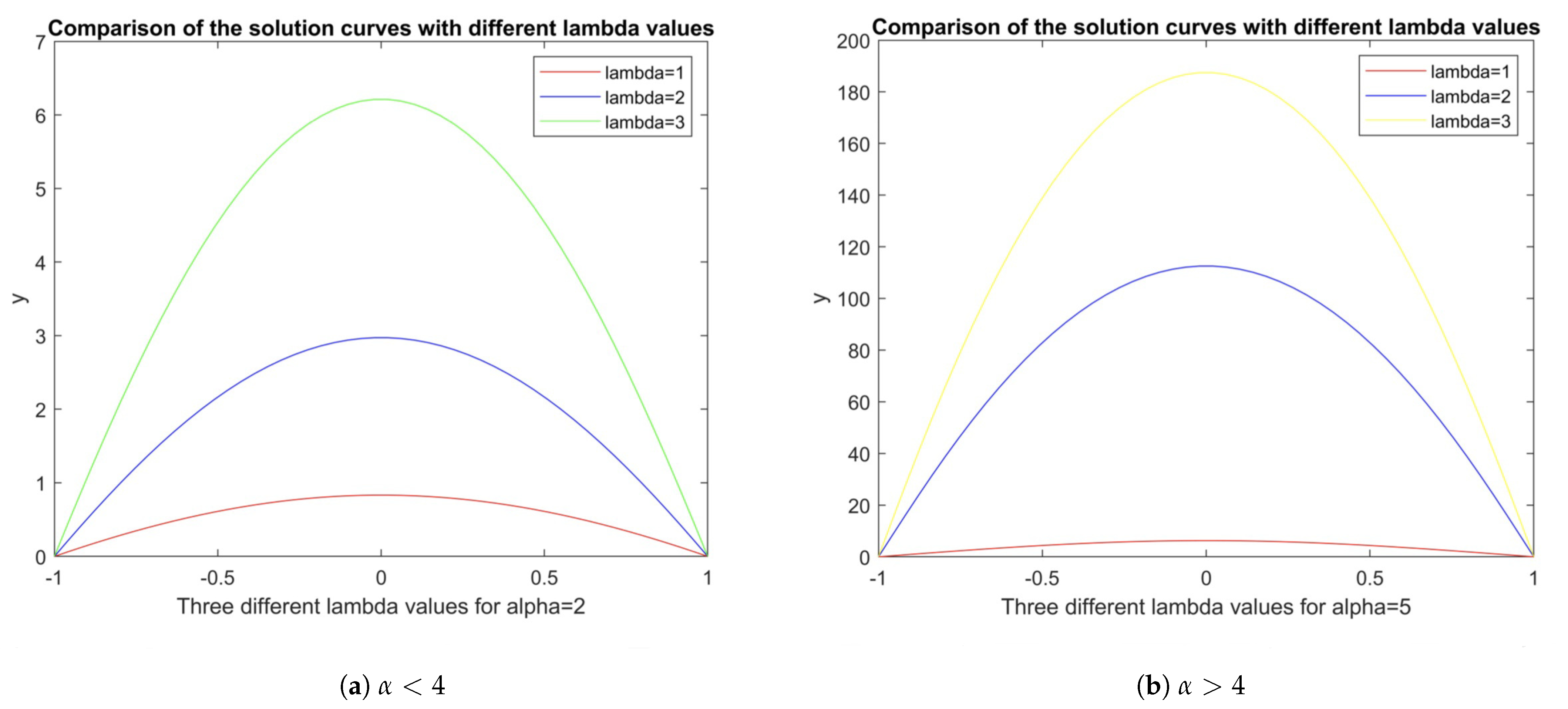
In this section, we produce some numerical solutions using Matlab to give some direct illustration for the solutions. Figure 1 shows that the order sequence of solutions follow the value of $\lambda$ as proved in Theorem 6. In both cases of $\alpha <4$ (Figure 1a) and $\alpha >4$ (Figure 1b), the order of the solutions follows the order of the parameter $\lambda$.

Figure 1. Order sequences for $\lambda$ values.

Lemma 2

([5], p. 479). If $u\left(t\right)$ is a solution of BVP (1.1), then $u\left(t\right)$ is symmetric about $t=0$. Thus, $u\left(t\right)=u(-t)$.

The following property on the norm and order of the solutions are new, to our knowledge.

Proposition 1.

If $u_1\left(t\right)$ and $u_2\left(t\right)$ are two solutions of BVP (1.1) for the same λ and $\parallel u_1\parallel >\parallel u_2\parallel$, then $u_1\left(t\right)>u_2\left(t\right)$ for $t\in (-1,1)$.

Proof. 

Since $u_1\left(t\right)$ and $u_2\left(t\right)$ are symmetric about $t=0$, it is sufficient to prove that $u_1\left(t\right)>u_2\left(t\right)$ for $t\in (-1,0]$. First, we prove that $u_1\left(t\right)\ge u_2\left(t\right)$ for $t\in (-1,0]$. Let $f\left(x\right)=exp\left(\frac{\alpha x}{\alpha +x}\right)$ for $x\ge 0$ and $F\left(u\right)={\int }_0^{u}f\left(s\right)ds$. From (1.1), we have

$$u^{″}{u}^{\prime }+\lambda f\left(u\right)u^{\prime }=0.$$

Integrating both sides from 0 to $u\left(t\right)$, we obtain

$$\frac{1}{2}{\left(u^{\prime }\left(t\right)\right)}^2+\lambda F\left(u\right)=C,$$

where C is a constant. Since $u\left(0\right)=\parallel u\parallel$ and $u^{\prime }\left(0\right)=0$, we find $C=\lambda F(\parallel u\parallel )$. Therefore,

$$\frac{1}{2}{\left(u^{\prime }\left(t\right)\right)}^2+\lambda F\left(u\right)=\lambda F(\parallel u\parallel ).$$

(16)

At $t=-1$, $u^{\prime }(-1)=\sqrt{2\lambda F(\parallel u\parallel )}$. Thus,

$$u_1^{\prime }(-1)=\sqrt{2\lambda F(\parallel u_1\parallel )}>\sqrt{2\lambda F(\parallel u_2\parallel )}=u_2^{\prime }(-1).$$

There exists an interval $(-1,c)$ such that $u_1\left(t\right)>u_2\left(t\right)$ for $t\in (-1,c)$. Suppose that $-1<r<0$ is the first value such that $u_1\left(r\right)=u_2\left(r\right)$ and $u_1\left(t\right)<u_2\left(t\right)$ for $t>r$ in an interval. Using (6.1), we have

$$\begin{array}{ccc}\hfill u_1^{\prime }\left(r\right)& =& \sqrt{2\lambda F(\parallel u_1\parallel )-2\lambda F\left(u_1\left(r\right)\right)}\hfill \\ & >& \sqrt{2\lambda F(\parallel u_2\parallel )-2\lambda F\left(u_2\left(r\right)\right)}=u_2^{\prime }\left(r\right).\hfill \end{array}$$

This is clearly a contradiction. Next, from the corresponding integral equation, we have

$$\begin{array}{ccc}\hfill u_1\left(t\right)& =& \frac{\lambda }{2}{\int }_{-1}^{1}G(s,t)exp\left(\frac{\alpha u_1\left(s\right)}{\alpha +u_1\left(s\right)}\right)ds\hfill \\ & >& \frac{\lambda }{2}{\int }_{-1}^{1}G(s,t)exp\left(\frac{\alpha u_2\left(s\right)}{\alpha +u_2\left(s\right)}\right)ds=u_2\left(t\right).\hfill \end{array}$$

The proof is complete. □

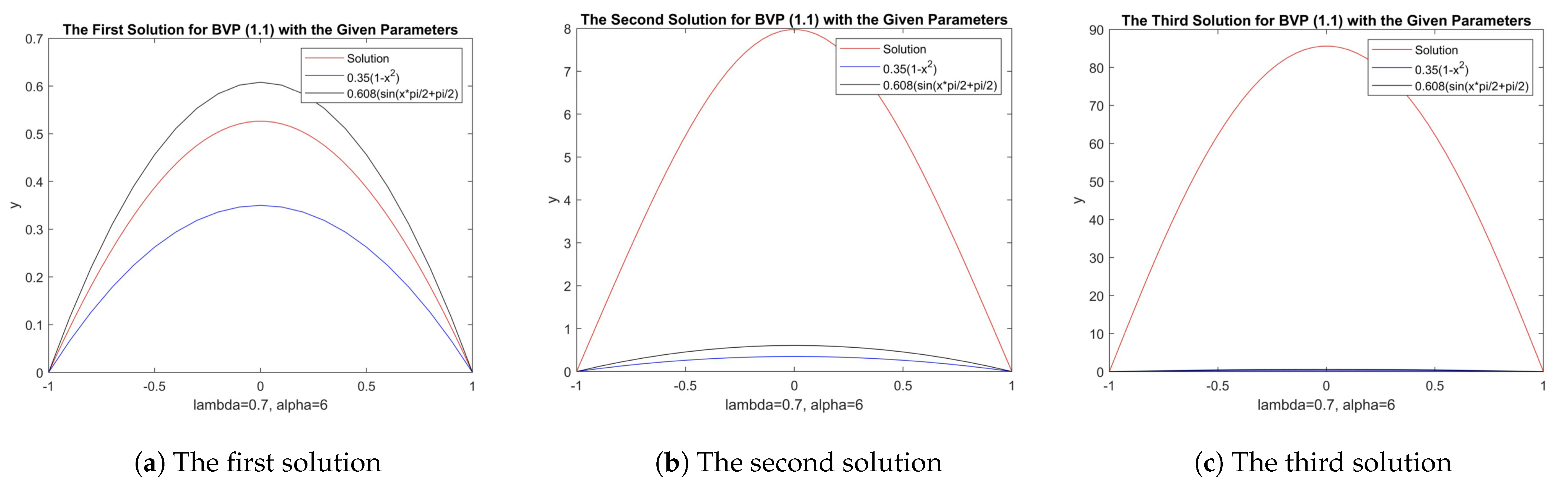
It is interesting to see that all three solutions were found, as shown in Figure 2, where $\alpha =6$ and $\lambda =0.7$. In addition, $\frac{\lambda }{2}=0.35$ and the value of b satisfying $\frac{0.7f\left(b\right)}{2b}=1$ is $0.608$. Figure 2a is consistent with Theorem 5. The value of $x_2=22.39$ and the solution curve in Figure 2c clearly supports the result in Theorem 7.

Figure 2. Three solutions.

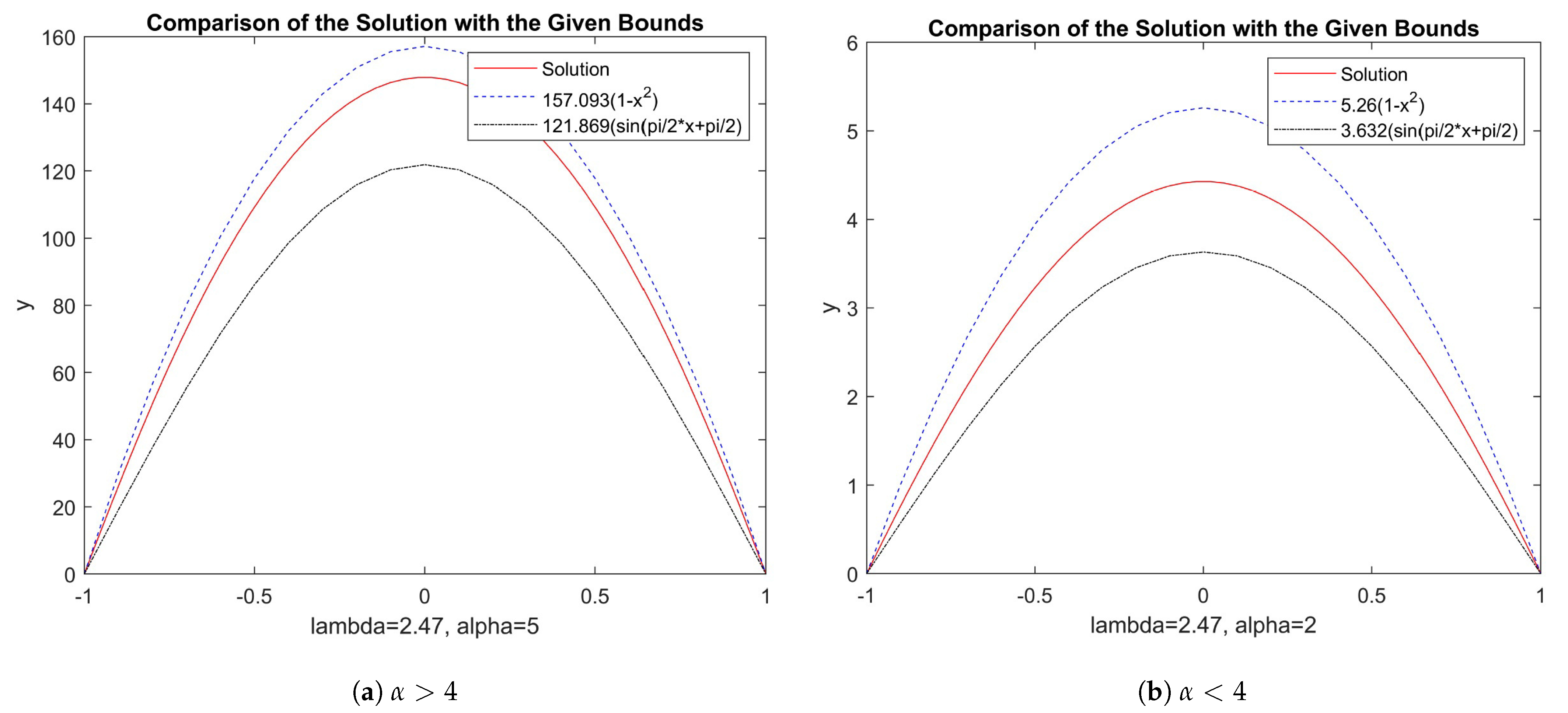
Remark 5.

When $\lambda >{\left(\frac{\pi }{2}\right)}^2\approx 2.4674$, combining Theorems 4 and 5, there exist solutions $u_1$ and $u_2$ such that

$$u_1\left(t\right)\le b(1-t^2)and{u}_2\left(t\right)\ge x_{0}sin(\frac{\pi }{2}t+\frac{\pi }{2}),$$

where the constant b satisfying $g\left(b\right)=\frac{2}{\lambda }$, $x_0$ is the smallest value satisfying $g\left(x_0\right)=1$. Since $\lambda \ge {\left(\frac{\pi }{2}\right)}^2$, $g\left(b\right)<g\left(x_0\right)$. Thus, $b>x_0$ because they must be values exceeding $x_2$ in Theorem 7 when $\alpha >4.$ If $\alpha \le 4$, g is decreasing. Assuming a unique solution exists, then $u_1=u_2=u$, and we have

$$x_{0}sin(\frac{\pi }{2}t+\frac{\pi }{2})\le u\left(t\right)\le b(1-t^2) if \lambda \ge {\left(\frac{\pi }{2}\right)}^2.$$

(17)

Figure 3 illustrates the upper bound and lower bound given by (17). In (A), the solution of BVP (1.1) for $\lambda =2.47\ge {\left(\frac{\pi }{2}\right)}^2$ and $\alpha =5>4.$ In this case, $x_0=121.869$ and $b=157.093$, and so $121.869sin(\frac{\pi }{2}t+\frac{\pi }{2})<u\left(t\right)<157.093(1-t^2).$ In (B), one calculated the solution of BVP (1.1) for $\lambda =2.47$ and $\alpha =2<4,$ In this case, $x_0=3.632$ and $b=5.26$ and so $3.632sin(\frac{\pi }{2}t+\frac{\pi }{2})<u\left(t\right)<3.26(1-t^2)$.

Figure 3. Upper and lower bounds for solutions.

Remark 6.

With the advantages of the concrete equation (1.1), we are able to obtain more detailed quantitative properties for the solutions as given in the above sections. The results provide ideas for solving similar problems for more abstract problems. For example, similar approaches may be applied to study parameter dependent operator equations in abstract partial ordered Banach spaces.

In conclusion, we studied a two-point boundary value problem arising from the combustion theory. The second-order system of differential equations involves two positive parameters $\lambda$ and $\alpha$ that are physically significant in the process.

Using topological methods, we proved results on uniqueness, existence, and multiplicity of positive solutions depending on the range of the two parameters. The results enriched previous work on this important application problem.

References

1. Bebernes, J.; Eberly, D. Mathematical Problems from Combustion Theory; Springer: New York, NY, USA, 1989. [Google Scholar]
2. Boddington, T.; Gray, P.; Robinson, C. Thermal explosion and the disappearance of criticality at small activation energies: Exact results for the slab. Proc. R. Soc. Lond. Ser. A Math. Phus. Eng. Sci. 1979, 368, 441–461. [Google Scholar]
3. Brown, K.J.; Ibrahim, M.M.A.; Shivaji, R. S-Shaped bifurcation curves. Nonlinear Anal. 1981, 5, 475–486. [Google Scholar] [CrossRef]
4. Hastings, S.P.; McLeod, J.B. The number of solutions to an equation from catalysis. Proc. R. Soc. Edinb. Sect. A 1985, 101, 213–230. [Google Scholar] [CrossRef]
5. Hung, K.C.; Wang, S.H. A theorem on S-shaped bifurcation curve for a positone problem with convex, concave nonlinearity and its applications to the perturbed Gelfand problem. J. Differ. Equ. 2011, 251, 223–237. [Google Scholar] [CrossRef] [Green Version]
6. Huang, S.Y.; Wang, S.H. On S-shaped bifurcation curves for a two-point boundary value problem arising in a theory of thermal explosion. Discret. Contin. Dyn. Syst. 2015, 35, 4839–4858. [Google Scholar] [CrossRef]
7. Huang, S.Y.; Wang, S.H. Proof of a conjecture for the one-dimensional perturbed Gelfand problem from combustion theory. Arch. Ration. Mech. Anal. 2016, 222, 769–825. [Google Scholar] [CrossRef]
8. Shivaji, R. Uniqueness results for a class of positone problems. Nonlinear Anal. 1983, 7, 223–230. [Google Scholar] [CrossRef]
9. Xing, H.; Chen, H.; Yao, R. Reversed S-shaped bifurcation curve for a Neumann problem. Discret. Dyn. Nat. Soc. 2018, 2018, 5376075. [Google Scholar] [CrossRef]
10. Xu, B.; Wang, Z. On S-shaped bifurcation curves for a class of perturbed semilinear equations. Chin. Ann. Math. B 2008, 29, 641–662. [Google Scholar] [CrossRef]
11. Wang, S.H. On S-shaped bifurcation curves. Nonlinear Anal. TMS 1994, 22, 1475–1485. [Google Scholar] [CrossRef]
12. Korman, P.; Li, Y. On the exactness of an S-Shaped bifurcation curve. Proc. Am. Math. Soc. 1999, 127, 1011–1020. [Google Scholar] [CrossRef] [Green Version]
13. Zhai, C.; Wang, F. ϕ-(h,e)-concave operators and applications. J. Math. Anal. Appl. 2017, 4543, 571–584. [Google Scholar] [CrossRef]
14. Feng, W.; Zhang, G. New fixed point theorems on order intervals and their applications. Fixed Point Theory Appl. 2015, 2015, 1–10. [Google Scholar] [CrossRef] [Green Version]
15. Zeidler, E. Nonlinear Functional Analysis and Its Application I; Springer: New York, NY, USA, 1986. [Google Scholar]
16. Zhai, C.; Wang, F. Properties of positive solutions for the operator equation Ax = λx and applications to fractional differential equations with integral boundary conditions. Adv. Differ. Equ. 2015, 366, 1–10. [Google Scholar]
Figure 1. Order sequences for λ values.
Symmetry 13 01606 g001