Control Problem Related to 2D Stokes Equations with Variable Density and Viscosity

Abstract

We study an optimal control problem for the stationary Stokes equations with variable density and viscosity in a 2D bounded domain under mixed boundary conditions. On in-flow and out-flow parts of the boundary, nonhomogeneous Dirichlet boundary conditions are used, while on the solid walls of the flow domain, the impermeability condition and the Navier slip condition are provided. We control the system by the external forces (distributed control) as well as the velocity boundary control acting on a fixed part of the boundary. We prove the existence of weak solutions of the state equations, by firstly expressing the fluid density in terms of the stream function (Frolov formulation). Then, we analyze the control problem and prove the existence of global optimal solutions. Using a Lagrange multipliers theorem in Banach spaces, we derive an optimality system. We also establish a second-order sufficient optimality condition and show that the marginal function of this control system is lower semi-continuous.

1. Introduction

In this work, we study an optimal control problem for the stationary Stokes equations with variable density and viscosity in a domain $\Omega \subset {\mathbb{R}}^2$, which is assumed to be a bounded and connected set with boundary $\Gamma \stackrel{\mathrm{def}}{=}\partial \Omega$ of class $C^1$. Specifically, we consider the following system of partial differential equations (PDEs):

$$\left\{\begin{array}{ccc}\hfill -\mathrm{div}[\mu \mathit{D}(\mathbf{u})]+\nabla \pi & =& \rho \mathbf{f}\mathrm{in}\Omega ,\hfill \\ \hfill \mathbf{u}·\nabla \rho & =& 0\mathrm{in}\Omega ,\hfill \\ \hfill \mathrm{div}\mathbf{u}& =& 0\mathrm{in}\Omega .\hfill \end{array}\right.$$

(1)

Here, the unknown functions are the velocity field $\mathbf{u}:\Omega \to {\mathbb{R}}^2$, the hydrostatic pressure $\pi :\Omega \to \mathbb{R}$, and the density $\rho :\Omega \to {\mathbb{R}}_{+}$ for a nonhomogeneous fluid that flows through the domain $\Omega$. The vector function $\mathbf{f}:\Omega \to {\mathbb{R}}^2$ represents a distributed control that acts on the motion equation and belongs to a closed and convex set $\mathcal{F}$; the function $\mu :\Omega \to {\mathbb{R}}_{+}$ describes the dynamic viscosity of the fluid; $\mathit{D}(\mathbf{u})$ is the symmetric part of the velocity gradient (the deformation rate tensor), i.e., $\mathit{D}(\mathbf{u})\stackrel{\mathrm{def}}{=}\frac{1}{2}(\nabla \mathbf{u}+{(\nabla \mathbf{u})}^{\top })$.

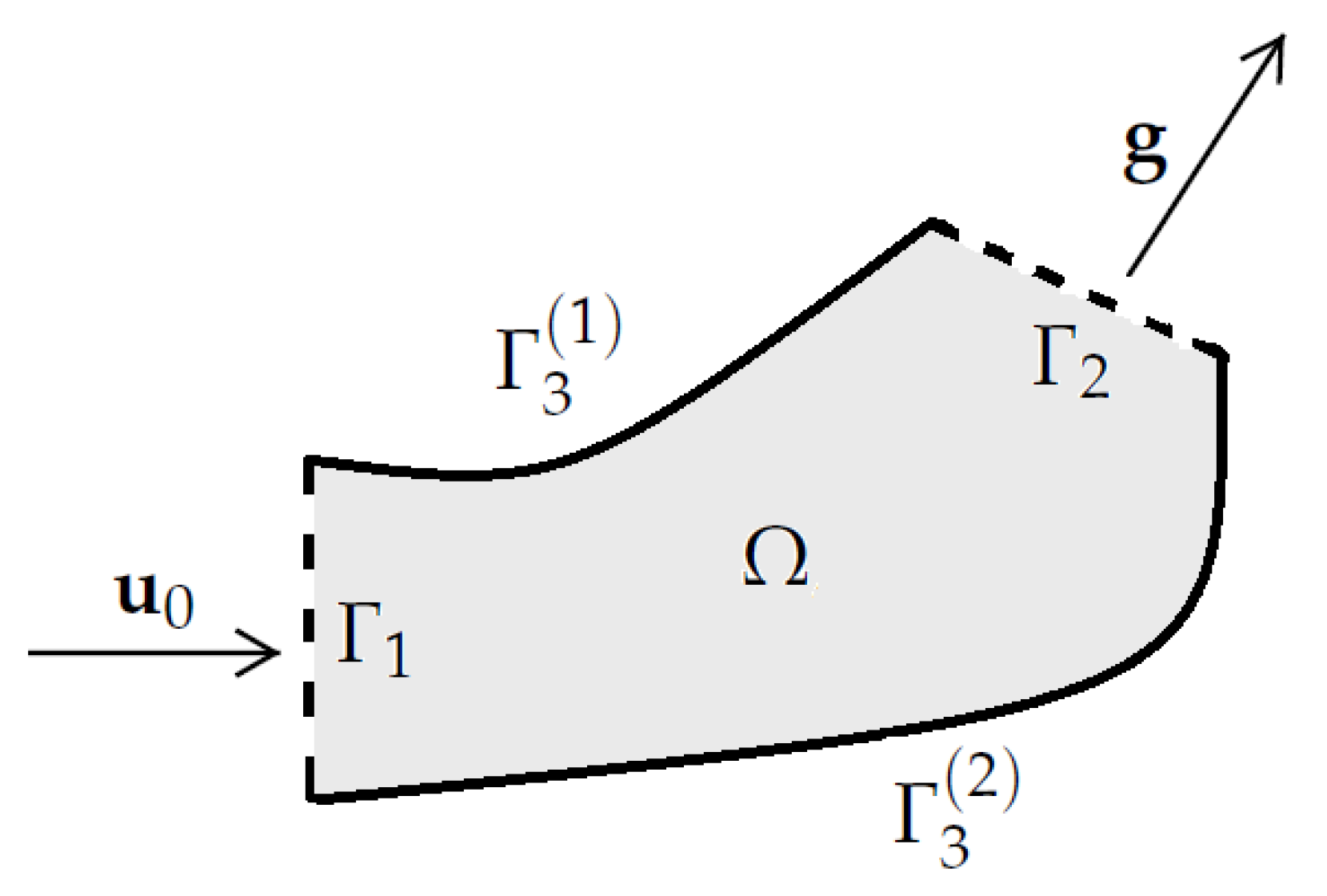
In order to describe boundary conditions for the velocity field and the density function in (1), we divide the boundary in three open disjoint parts: $\Gamma ={\overline{\Gamma }}_1\cup {\overline{\Gamma }}_2\cup {\overline{\Gamma }}_3$, where ${\Gamma }_1$ and ${\Gamma }_2$ are in-flow/out-flow parts and ${\Gamma }_3=\Gamma \backslash ({\overline{\Gamma }}_1\cup {\overline{\Gamma }}_2)$ is the lateral part (solid walls) of the boundary. Then, we impose the following boundary conditions:

$$\begin{array}{ccc}\hfill \mathbf{u}& =& {\mathbf{u}}_{\mathbf{g}}\stackrel{\mathrm{def}}{=}\left\{\begin{array}{cc}\hfill {\mathbf{u}}_0& \mathrm{on}{\Gamma }_1,\\ \hfill \mathbf{g}& \mathrm{on}{\Gamma }_2,\end{array}\right.\hfill \end{array}$$

(2)

$$\begin{array}{ccc}\hfill \rho & =& {\rho }_0>0\mathrm{on}{\Gamma }_1.\hfill \end{array}$$

(3)

The functions ${\rho }_0$ and ${\mathbf{u}}_0$ are defined on ${\Gamma }_1$ and describe a Dirichlet boundary condition. The function $\mathbf{g}$ describes a Dirichlet boundary control for $\mathbf{u}$ on ${\Gamma }_2$ and belongs to a closed convex set ${\mathcal{G}}_{{\mathbf{u}}_0}$.

Additionally, we assume the following:

$$\begin{array}{ccc}& & {\Gamma }_1\mathrm{is} \mathrm{an} \mathrm{arcwise} \mathrm{connected} \mathrm{and} \mathrm{closed} \mathrm{set} \mathrm{on} \Gamma \mathrm{with} |{\Gamma }_1|>0;\hfill \end{array}$$

(4)

$$\begin{array}{ccc}& & \mathrm{either} {\mathbf{u}}_0·\mathbf{n}>0\mathrm{on} {\Gamma }_1(\mathrm{out}-\mathrm{flow}) \mathrm{or} {\mathbf{u}}_0·\mathbf{n}<0\mathrm{on} {\Gamma }_1(\mathrm{in}-\mathrm{flow}),\hfill \end{array}$$

(5)

where $|{\Gamma }_1|$ denotes the length of the curve ${\Gamma }_1$ and $\mathbf{n}$ is the outward unit normal vector to the curve $\Gamma$. Observe that condition (5) implies that ${\Gamma }_1$ is either a part of the boundary where the fluid flows outward or a part where the fluid flows inward.

An example of the flow domain $\Omega$ is given in Figure 1.

Figure 1. The flow domain $\Omega$ with boundary $\Gamma ={\overline{\Gamma }}_1\cup {\overline{\Gamma }}_2\cup {\overline{\Gamma }}_3$, where ${\Gamma }_3={\Gamma }_3^{(1)}\cup {\Gamma }_3^{(2)}$.

Finally, on the part ${\Gamma }_3$ we impose the impermeability condition and the Navier slip condition:

$$\mathbf{u}·\mathbf{n}=0\mathrm{and}{[\mu \mathit{D}(\mathbf{u})\mathbf{n}+\alpha \mathbf{u}]}_{\mathrm{tang}}=\mathbf{0}.$$

(6)

The term ${[\mu \mathit{D}(\mathbf{u})\mathbf{n}+\alpha \mathbf{u}]}_{\mathrm{tang}}$ is the tangential component of the vector $\mu \mathit{D}(\mathbf{u})\mathbf{n}+\alpha \mathbf{u}$; that is,

$${[\mu \mathit{D}(\mathbf{u})\mathbf{n}+\alpha \mathbf{u}]}_{\mathrm{tang}}\stackrel{\mathrm{def}}{=}\mu \mathit{D}(\mathbf{u})\mathbf{n}+\alpha \mathbf{u}-[(\mu \mathit{D}(\mathbf{u})\mathbf{n}+\alpha \mathbf{u})·\mathbf{n}]\mathbf{n}.$$

For the sake of brevity, the nonhomogeneous Stokes system (1) with mixed boundary conditions (2), (3), (6) will be referred to as problem NS-MBC in what follows.

The Navier slip boundary condition was proposed by Navier [1]; it is based on a balance between the fluid velocity tangent to the surface and the rate of strain at the boundary, i.e., the tangential component of the viscous stress at the boundary should be proportional to the tangential velocity. The components of the normal velocity to the surface is naturally zero, as mass cannot penetrate an impermeable solid surface. This type of boundary condition is involved when one studies boundary layer problems, such as in channels or Couette flows and is well justified by Jäger-Mikelić [2,3]. In addition, the real number $\alpha \ge 0$ is the friction coefficient, which measures the tendency of the fluid to slip on the part ${\Gamma }_3$. When $\alpha =0$, the fluid slips on ${\Gamma }_3$ without friction and there are no boundary layers, while if $\alpha$ goes to $+\infty$, then the friction is so intense that the fluid is almost at rest near the boundary [4] (see also [5]). Thus, from the physical point of view, boundary conditions (6) make more sense than the classical Dirichlet boundary conditions.

Moreover, in order to define a correct variational formulation (weak solutions concept) of problem NS-MBC, the classical Green identities are not applicable in this case. The above leads us to study other results of integration by parts (see Lemma 1, below). Additionally, in order to correctly control the ${\mathbf{H}}_{\sigma }$-norm in terms of the ${\mathbf{L}}^2$-norm of the deformation rate tensor, i.e., the norm ${\Vert \mathit{D}(\mathbf{u})\Vert }^2$, we must employ the Korn inequality (see [6], p. 52), which is not usual.

Some examples of flow phenomena that might require the introduction of a Navier slip boundary condition have been presented by Fujita [7,8], namely: a drainage or canal in which its bottom is covered with a layer of mud and pebbles; the blood flow in the vein of a patient suffering from arterial sclerosis; an avalanche of water and rocks; a flow of iron coming out of a smelting. Some other applications can be consulted in [9,10,11].

It is well known that fluids in which the density and viscosity are variable have several important applications, both in natural phenomena as well as in industry. These fluids present a wider range of interesting phenomena, compared to fluids with constant density and viscosity (also called homogeneous fluids), and there are several mathematical models that describe different physical situations. In particular, some examples of the physical modeling of mixtures of incompressible fluids can be found in [12] and the respective mathematical analysis of these models were developed in [13,14,15]. We emphasize that all these works only consider fluids with constant viscosity and Dirichlet boundary conditions. Furthermore, as far as we know, there are no previous studies on the existence of weak solutions of problem NS-MBC, and analyses of optimal control problems have not been carried out either.

The above motivates the analysis of problem NS-MBC. The main mathematical difficulty that arises in the study of this problem in relation to the Stokes system with variable density and viscosity is due to several nonlinearities in the problem ($-\mathrm{div}[\mu \mathit{D}(\mathbf{u})]$, $\rho \mathbf{f}$ in Equation (1)₁ and $\mathbf{u}·\nabla \rho$ in Equation (1)₂), which, due to the product with the unknown density and viscosity, are much harder to deal with than the corresponding terms ones appearing in the Stokes equations in which the density and viscosity are known constants. Moreover, since the nonlinearity of the term $\mathbf{u}·\nabla \rho$ is not related to a monotone operator, we must work with arguments that are different than what is typical when dealing with elliptic or parabolic problems and nonlinearities and restrictions related to monotone operators. To overcome these difficulties, we will use the stream formulation presented by Frolov [16] that is, the fluid density is represented in terms of its stream function through another function determined by the boundary conditions. This representation allows us to drop the continuity equation, which facilitates the introduction of the weak solution concept of problem NS-MBC. The stream formulation was used in [17,18,19,20,21].

The purpose of this work is to study an optimal control problem related to weak solutions of problem NS-MBC. We would like to point out that the literature to the mathematical analysis of optimal control problems associated with systems of partial differential equations modeling the motion of viscous incompressible fluids with variable density and viscosity is scarce. The main difficulty lies in the mathematical handling. In fact, the systems that model the behavior of viscous and incompressible fluids with constant density can have two types of character: either elliptical, for the steady state, or parabolic, for the non-stationary state. In both cases, when an approximation argument is used, such as the Galerkin method, for instance, higher-order estimates are usually obtained for the approximate solutions, which facilitates the passage to the limit in the nonlinear terms and, consequently, it is more simple to achieve the required results. On the other hand, for systems that model the motion of fluids with variable density, the equations that compose the system present nonlinearities that are more difficult to handle since they makes it impossible to obtain higher-order estimates and make it difficult to pass to the limit in the nonlinear terms. The system of equations that we have considered in our work (problem NS-MBC), the first equation of system (1) has an elliptic character but is coupled with a first-order transport equation for the density $\rho$ (see Equation (1)₁), which gives a hyperbolic character to the model. These drawbacks make it difficult to obtain estimates with high regularity and increase the difficulties in passing to the limit.

Let us mention the available literature on the analysis of optimal control problems for nonhomogeneous fluid flows. The beginning of the study of such problems dates back to the paper of Illarionov [17]. He investigated optimal boundary control for a model of 2D steady-state flows of a nonhomogeneous incompressible fluid under the assumption that the viscosity $\mu$ is constant. Using the external forces field as a control function, Mallea-Zepeda et al. [19] proved the existence of optimal solutions to this model and obtained the first-order necessary optimality conditions. Boundary control for a 2D stationary system of micropolar fluid with variable density was studied in [20]. Certain classes of optimal control problems for the 2D Boussinesq equations with variable density and constant viscosity are analyzed in [21].

We also mention that there is a large number of mathematical works devoted to the study of optimal control problems for PDEs describing flows of a homogeneous fluid (see, for example, refs. [22,23,24,25,26] and the numerous references therein). Such problems are currently fairly well understood, while control and optimization problems for nonhomogeneous fluid flows remain a serious challenge. Motivated by this fact, we performed our study, which can be considered a starting point for future investigations of non-Newtonian fluid models, where more general inhomogeneities can be analyzed.

The outline of the present paper is as follows: In Section 2, we fix the notation, introduce the function spaces to be used and establish the concept of weak solutions of problem NS-MBC, using the stream formulation. In Section 3, we prove the existence and uniqueness of weak solutions of system NS-MBC, in order to establish that the admissible solutions set is nonempty (see (39) below). In Section 4, we introduce the optimal control problem to this system and prove the existence of global optimal solutions. Moreover, using a Lagrange multipliers theorem in Banach spaces, we derive an optimality system, and, establishing a coercivity condition for the Lagrangian function, we obtain a second-order sufficient optimality condition. Finally, we show that the marginal function related to this control system is lower semi-continuous with respect to the one-sided Hausdorff distance.

For the reader’s convenience, in Appendix A (see Table A1), we collect the main symbols used in this paper and explain their meaning.

2. Preliminaries

In this section, we introduce the notation, function spaces and principal results that we will use throughout the work.

2.1. Notation and Function Spaces

Let E be a Banach space. By $2^E$ we denote the collection of all subsets of E (the power set of E). By definition, put

$$\begin{array}{cc}\hfill {\mathcal{P}}_{\mathrm{b}}\left[E\right]\stackrel{\mathrm{def}}{=}& \left\{M\in 2^E\backslash \{⌀\}:M\mathrm{is} \mathrm{bounded}\right\},\hfill \\ \hfill {\mathcal{P}}_{\mathrm{c}}\left[E\right]\stackrel{\mathrm{def}}{=}& \left\{M\in 2^E\backslash \{⌀\}:M\mathrm{is} \mathrm{convex}\right\},\hfill \\ \hfill {\mathcal{P}}_{\mathrm{cl}}\left[E\right]\stackrel{\mathrm{def}}{=}& \left\{M\in 2^E\backslash \{⌀\}:M\mathrm{is} \mathrm{closed}\right\}\hfill \end{array}$$

and

$${\mathcal{P}}_{\mathrm{c},\mathrm{cl}}\left[E\right]\stackrel{\mathrm{def}}{=}{\mathcal{P}}_{\mathrm{c}}\left[E\right]\cap {\mathcal{P}}_{\mathrm{cl}}\left[E\right],{\mathcal{P}}_{\mathrm{b},\mathrm{c},\mathrm{cl}}\left[E\right]\stackrel{\mathrm{def}}{=}{\mathcal{P}}_{\mathrm{b}}\left[E\right]\cap {\mathcal{P}}_{\mathrm{c}}\left[E\right]\cap {\mathcal{P}}_{\mathrm{cl}}\left[E\right].$$

Let $\mathcal{U}$ and $\mathcal{W}$ be subsets of E. By $d_E(\mathcal{U},\mathcal{W})$ we denote the one-sided Hausdorff distance from the set $\mathcal{U}$ to the set $\mathcal{W}$, that is,

$$d_E(\mathcal{U},\mathcal{W})\stackrel{\mathrm{def}}{=}\underset{u\in \mathcal{U}}{sup}\underset{w\in \mathcal{W}}{inf}{\Vert u-w\Vert }_E.$$

For $m\in \mathbb{N}$ and $1\le p\le +\infty$, we will use the Sobolev space $H^m(\Omega )\stackrel{\mathrm{def}}{=}{W}^{m,2}(\Omega )$ and the Lebesgue space $L^p(\Omega )$ with norms denoted by ${\Vert ·\Vert }_{H^m}$ and ${\Vert ·\Vert }_{L^p}$, respectively. In particular, when $p=2$, $L^2(\Omega )$ is a Hilbert space; in this case, the $L^2$-norm and $L^2$-scalar product are represented by $\Vert ·\Vert$ and $(·,·)$, respectively. In addition, the $L^p(\Gamma )$-norm is denoted by ${\Vert ·\Vert }_{L^p(\Gamma )}$. The corresponding spaces of vector-valued functions are denoted by bold script; for instance, ${\mathbf{H}}^1(\Omega )$, ${\mathbf{L}}^p(\Omega )$, and so on. Recall that the restriction of a function $v\in H^1(\Omega )$ to the curve $\Gamma$ is defined by the formula ${v|}_{\Gamma }\stackrel{\mathrm{def}}{=}{\gamma }_{0}v$, where ${\gamma }_0:H^1(\Omega )\to L^p(\Gamma )$ is the trace operator (see [27], § 2.4.2).

We also use the following divergence-free Banach spaces (solenoidal spaces):

• The space ${\mathbf{H}}_{\sigma }\stackrel{\mathrm{def}}{=}\{\mathbf{v}\in {\mathbf{H}}^1(\Omega ):\mathrm{div}\mathbf{v}=0\mathrm{in} \Omega \mathrm{and} \mathbf{v}·\mathbf{n}=0 \mathrm{on} {\Gamma }_3\}$ equipped with the usual norm and scalar product of ${\mathbf{H}}^1(\Omega )$;
• The space ${\mathbf{V}}_{\sigma }\stackrel{\mathrm{def}}{=}\{\mathbf{v}\in {\mathbf{H}}_{\sigma }:\mathbf{v}=\mathbf{0} \mathrm{on} \Gamma \backslash {\Gamma }_3\},$ which is a Hilbert space with the scalar product ${(\mathbf{v},\mathbf{w})}_{{\mathbf{V}}_{\sigma }}\stackrel{\mathrm{def}}{=}(\mathit{D}(\mathbf{v}),\mathit{D}(\mathbf{w}))$ and the norm ${\Vert \mathbf{v}\Vert }_{{\mathbf{V}}_{\sigma }}\stackrel{\mathrm{def}}{=}\Vert \mathit{D}(\mathbf{v})\Vert$.

By $C^l(\Omega )$ (resp. $C^l(\mathbb{R})$) we denote the Banach space of functions that are l times continuously differentiable on $\Omega$ (resp. on $\mathbb{R}$) and by $C_b^l(\Omega )$ (resp. $C_b^l(\mathbb{R})$) the space of l times continuously differentiable and bounded functions on $\Omega$ (resp. on $\mathbb{R}$).

Moreover, if X is a general Banach space, its dual topological is denoted by $X^{\prime }$ and the pairing duality by ${⟨·,·⟩}_{X^{\prime }}$ or $⟨·,·⟩$, when this does not lead to ambiguities. In particular, ${\mathbf{H}}_{\sigma }^{\prime }$ denotes the dual of ${\mathbf{H}}_{\sigma }$, and ${\mathbf{V}}_{\sigma }^{\prime }$ denotes the dual of ${\mathbf{V}}_{\sigma }$.

Furthermore, the space of the traces of vector functions from ${\mathbf{H}}^1(\Omega )$ is defined by

$${\mathbf{H}}^{1/2}(\Gamma )\stackrel{\mathrm{def}}{=}\{\mathbf{h}\in {\mathbf{L}}^2(\Gamma ):\mathrm{there} \mathrm{exists} \mathbf{v}\in {\mathbf{H}}^1(\Omega )\mathrm{such} \mathrm{that} \mathbf{v}{|}_{\Gamma }=\mathbf{h}\}$$

with the norm ${\Vert \mathbf{h}\Vert }_{{\mathbf{H}}^{1/2}(\Gamma )}\stackrel{\mathrm{def}}{=}{\Vert {\mathbf{L}}_{\Omega }\mathbf{h}\Vert }_{{\mathbf{H}}^1(\Omega )},$ where ${\mathbf{L}}_{\Omega }:{\mathbf{H}}^{1/2}(\Gamma )\to {\mathbf{H}}^1(\Omega )$ is the lifting (trace extension) operator such that ${\gamma }_0\circ {\mathbf{L}}_{\Omega }=\mathbf{Id}$ (see, for example, ref. [28], Chapter III, Theorem III.2.22).

The dual space of ${\mathbf{H}}^{1/2}(\Gamma )$ is denoted by ${\mathbf{H}}^{-1/2}(\Gamma )$, and the respective duality product is denoted by ${⟨·,·⟩}_{\Gamma }$.

For a subset $\mathcal{S}$ of $\Gamma$, we introduce the subspace ${\mathbf{H}}_0^{1/2}(\mathcal{S})$ as follows:

$${\mathbf{H}}_0^{1/2}(\mathcal{S})\stackrel{\mathrm{def}}{=}\{\mathit{\phi }\in {\mathbf{L}}^2(\mathcal{S}):\mathrm{there} \mathrm{exists} \mathbf{w}\in {\mathbf{H}}^{1/2}{(\Gamma ) \mathrm{such} \mathrm{that} \mathbf{w}|}_{\mathcal{S}}=\mathit{\phi } \mathrm{and} \mathbf{w}{|}_{\Gamma \backslash \mathcal{S}}=\mathbf{0}\}.$$

Note that the injection ${\mathbf{H}}_0^{1/2}(\mathcal{S})\hookrightarrow {\mathbf{L}}^2(\mathcal{S})$ is continuous; that is, there exists a positive constant C which depends only on $\Omega$ such that ${\Vert \mathit{\phi }\Vert }_{{\mathbf{L}}^2(\mathcal{S})}\le C{\Vert \mathit{\phi }\Vert }_{{\mathbf{H}}_0^{1/2}(\mathcal{S})}$ (see [27], § 2.4.2).

The letter C denotes a positive constant, independent of the state $(\mathbf{u},\pi ,\rho )$ and the control $(\mathbf{f},\mathbf{g})$, but its value may change from line to line.

2.2. Weak Solutions

Let us assume that the following conditions are fulfilled:

$$\begin{array}{cc}\hfill & \mathbf{f}\in {\mathbf{L}}^2(\Omega ),{\mathbf{u}}_0\in {\mathbf{H}}_0^{1/2}({\Gamma }_1),\mathbf{g}\in {\mathbf{H}}_0^{1/2}({\Gamma }_2),\mu \in C^0(\overline{\Omega }),{\rho }_0\in C^0({\Gamma }_1),\eta \in C_b^0(\mathbb{R}),\phantom{{\int }_A^A}\hfill \end{array}$$

(7)

$$\begin{array}{cc}\hfill & \mathrm{there} \mathrm{exists} \mathrm{constants} {\mu }_{\ast }\mathrm{and} {\mu }^{\ast }\mathrm{such} \mathrm{that} 0<{\mu }_{\ast }\le \mu (\mathbf{x})\le {\mu }^{\ast }, \mathrm{for} \mathrm{any} \mathbf{x}\in \Omega ,\hfill \end{array}$$

(8)

$${\int }_{{\Gamma }_1}{\mathbf{u}}_0·\mathbf{n}+{\int }_{{\Gamma }_2}\mathbf{g}·\mathbf{n}=0.$$

(9)

To define the concept of weak solutions of problem NS-MBC, following the ideas of Frolov [16] (see, also [17,18,19,20,21], for more details), we express the fluid density in terms of the stream function. Namely, assuming conditions (4) and (5), we can express the fluid density as follows:

$$\rho (\mathbf{x})=\eta (\psi (\mathbf{x}))=\eta (N\mathbf{u})(\mathbf{x}),\forall \mathbf{x}\in \Omega ,$$

(10)

where $\eta$ is a function from the space $C_b^0(\mathbb{R})$, and $N:{\mathbf{H}}_{\sigma }\to H^2(\Omega )$ is the linear and continuous operator (see [17], Lemma 2.1) that takes each vector function $\mathbf{u}\in {\mathbf{H}}_{\sigma }$ to a function $\psi$ (stream function) such that

$$\mathrm{curl}(\psi {\overrightarrow{\mathbf{e}}}_3)=\overrightarrow{\mathbf{u}} \mathrm{in} \Omega ,\psi (\mathbf{x})={\int }_{{\Gamma }_1({\mathbf{x}}_0,\mathbf{x})}\mathbf{u}·\mathbf{n},\forall \mathbf{x}\in {\Gamma }_1,$$

(11)

where ${\overrightarrow{\mathbf{e}}}_3\stackrel{\mathrm{def}}{=}(0,0,1)$, $\overrightarrow{\mathbf{u}}\stackrel{\mathrm{def}}{=}(u_1,u_2,0)$, ${\mathbf{x}}_0$ is the initial point of the curve ${\Gamma }_1$, and ${\Gamma }_1({\mathbf{x}}_0,\mathbf{x})$ is the portion of ${\Gamma }_1$ lying between the points ${\mathbf{x}}_0$ and $\mathbf{x}$. In the Cartesian coordinate system, the first equality of (11) is equivalent to

$$\frac{\partial \psi }{\partial x_1}=-u_2,\frac{\partial \psi }{\partial x_2}=u_1\mathrm{in}\Omega .$$

(12)

For any $\eta \in C_b^1(\mathbb{R})$, the velocity field $\mathbf{u}$ and the density $\rho$, defined as in (10), satisfy relation (1)₂. Indeed, using the chain rule and (12), we obtain

$$\frac{\partial \rho }{\partial x_i}={\eta }^{\prime }(\psi )\frac{\partial \psi }{\partial x_i}=\left\{\begin{array}{c}-{\eta }^{\prime }(\psi )u_2\mathrm{if} i=1,\hfill \\ {\eta }^{\prime }(\psi )u_1\mathrm{if} i=2,\hfill \end{array}\right.$$

where ${\eta }^{\prime }$ denotes the first derivative of $\eta$. Therefore, we obviously have

$$\begin{array}{cc}\hfill \mathbf{u}·\nabla \rho =& u_1\frac{\partial \rho }{\partial x_1}+u_2\frac{\partial \rho }{\partial x_2}\hfill \\ \hfill =& -u_1{\eta }^{\prime }(\psi )u_2+u_2{\eta }^{\prime }(\psi )u_1=0\mathrm{in}\Omega .\hfill \end{array}$$

Note also that if $\eta \in C_b^0(\mathbb{R})$, then condition (1)₂ is satisfied at least in the weak sense, that is,

$${\int }_{\Omega }(\mathbf{u}·\nabla \omega )\rho =0,\forall \omega \in H^1(\Omega ) \mathrm{with} \omega =0 \mathrm{on} \Gamma .$$

This identity is not difficult to establish by applying the procedure of regularization for the function $\eta$ and passage to the limit.

Now it remains to choose a function $\eta$ so that the density function $\rho$ satisfies boundary condition (3). To this end, we introduce the function ${\psi }_0:{\Gamma }_1\to \mathbb{R}$ by the following formula:

$${\psi }_0(\mathbf{x})\stackrel{\mathrm{def}}{=}{\int }_{{\Gamma }_1({\mathbf{x}}_0,\mathbf{x})}{\mathbf{u}}_0·\mathbf{n},\forall \mathbf{x}\in {\Gamma }_1.$$

Clearly, ${\psi }_0\in C^0({\Gamma }_1)$. Moreover, from conditions (4) and (5) it follows that ${\psi }_0$ is strictly monotone on the curve ${\Gamma }_1$, and hence, there exists the inverse function ${\psi }_0^{-1}\in C^0(\mathcal{I})$, where $\mathcal{I}\stackrel{\mathrm{def}}{=}\{{\psi }_0(\mathbf{x}):\mathbf{x}\in {\Gamma }_1\}$. Therefore, if conditions (4) and (5) hold, ${\mathbf{u}}_0\in {\mathbf{H}}_0^{1/2}({\Gamma }_1)$, ${\rho }_0\in C^0({\Gamma }_1)$, and ${\rho }_0>0$ on ${\Gamma }_1$, then there exists a function $\eta \in C^0(\mathbb{R})$ such that

$$\eta (s)>0,\forall s\in \mathbb{R},\mathrm{and}\eta (s)={\rho }_0({\psi }_0^{-1}(s)),\forall s\in \mathcal{I}.$$

(13)

In the sequel, we assume that the function $\eta$ satisfying (13) is fixed.

Let us show that boundary condition (3) is satisfied. Indeed, taking into account (10) and (13), we obtain

$$\begin{array}{cc}\hfill \rho (\mathbf{x})=\eta (N\mathbf{u})(\mathbf{x})=& \rho \left({\int }_{{\Gamma }_1({\mathbf{x}}_{\mathbf{0}},\mathbf{x})}\mathbf{u}·\mathbf{n}\right)\hfill \\ \hfill =& \rho \left({\int }_{{\Gamma }_1({\mathbf{x}}_{\mathbf{0}},\mathbf{x})}{\mathbf{u}}_0·\mathbf{n}\right)\hfill \\ \hfill =& \rho \left({\psi }_0(\mathbf{x})\right)\hfill \\ \hfill =& {\rho }_0\left({\psi }_0^{-1}\left[{\psi }_0(\mathbf{x})\right]\right)\hfill \\ \hfill =& {\rho }_0(\mathbf{x}),\hfill \end{array}$$

for any $\mathbf{u}\in {\mathbf{H}}_{\sigma }$ such that $\mathbf{u}={\mathbf{u}}_0$ on ${\Gamma }_1$ and for all $\mathbf{x}\in {\Gamma }_1$.

Remark 1.

If the curve ${\Gamma }_1$ is of class $C^k$ and the following inclusions hold,

$${\rho }_0\in C^k({\Gamma }_1),{\mathbf{u}}_0·\mathbf{n}\in C^{k-1}({\Gamma }_1)$$

with $k\ge 1$; then there exists a function $\eta \in C^k(\mathbb{R})$ satisfying relations (13) (see [17]).

To obtain the weak formulation of problem NS-MBC, as usual, we take the ${\mathbf{L}}^2$-scalar product of equality (1)₁ with a test function $\mathbf{v}\in {\mathbf{V}}_{\sigma }$. Next, we use the relation $(\nabla \pi ,\mathbf{v})=0$ and the following result on integration by parts:

Lemma 1

(see [29]). Suppose that a vector function $\mathbf{u}\in {\mathbf{H}}^2(\Omega )$ satisfies boundary conditions (6), a vector function $\mathbf{v}\in {\mathbf{H}}^1(\Omega )$ satisfies the condition $\mathbf{v}·\mathbf{n}=0$ on Γ, and $\mu \in C^1(\overline{\Omega })$. Then, we have

$$-{\int }_{\Omega }\mathrm{div}\left[\mu \mathit{D}(\mathbf{u})\right]·\mathbf{v}={\int }_{\Omega }\mu \mathit{D}(\mathbf{u}):\mathit{D}(\mathbf{v})+\alpha {\int }_{\Gamma }\mathbf{u}·\mathbf{v},$$

where the symbol: denotes the component-wise product of matrices.

Thus, we arrive at the following definition of weak solutions to system NS-MBC.

Definition 1

(Weak solution). We say that a pair $(\mathbf{u},\rho )$ is a weak solution of problem NS-MBC if $\mathbf{u}\in {\mathbf{H}}_{\sigma }$, $\rho =\eta (N\mathbf{u})$ and the following weak formulation holds:

$$\left\{\begin{array}{ccc}\hfill {\displaystyle (\mu \mathit{D}(\mathbf{u}),\mathit{D}(\mathbf{v}))+\alpha {\int }_{{\Gamma }_3}\mathbf{u}·\mathbf{v}}& =& {⟨\mathbf{F}(\mathbf{u}),\mathbf{v}⟩}_{{\mathbf{V}}_{\sigma }^{\prime }},\forall \mathbf{v}\in {\mathbf{V}}_{\sigma },\hfill \\ \hfill \eta (N\mathbf{u})& =& {\rho }_0\mathrm{on} {\Gamma }_1,\hfill \\ \hfill \mathbf{u}& =& {\mathbf{u}}_{\mathbf{g}}\mathrm{on} \Gamma \backslash {\Gamma }_3,\hfill \end{array}\right.$$

(14)

where the operator $\mathbf{F}:{\mathbf{H}}_{\sigma }\to {\mathbf{V}}_{\sigma }^{\prime }$ is defined by $\mathbf{F}(\mathbf{u})\stackrel{\mathrm{def}}{=}\eta (N\mathbf{u})\mathbf{f}.$

3. Existence and Uniqueness of Weak Solutions

In this section, using the Schauder fixed-point theorem, we prove the existence and uniqueness of weak solutions of system NS-MBC; as far as we know, there are no previous results on the existence of weak solutions of this problem.

In order to prove the existence of a solution of (14), we reduce this problem to a new problem with homogeneous boundary conditions in terms of new unknown $\widehat{\mathbf{u}}$. The following result allows us to make the desired reduction.

Lemma 2

(see [20], Lemma 2). Suppose ${\mathbf{u}}_0\in {\mathbf{H}}_0^{1/2}({\Gamma }_1)$, $\mathbf{g}\in {\mathbf{H}}_0^{1/2}({\Gamma }_2)$, and equality (9) holds. Then, there exists a vector field ${\mathbf{u}}^e\in {\mathbf{H}}_{\sigma }$ such that ${\mathbf{u}}^e={\mathbf{u}}_0$ on ${\Gamma }_1$, ${\mathbf{u}}^e=\mathbf{g}$ on ${\Gamma }_2$ and ${\mathbf{u}}^e=\mathbf{0}$ on ${\Gamma }_3$, and satisfies the following estimate:

$$\Vert {\mathbf{u}}^e{\Vert }_{{\mathbf{H}}_{\sigma }}\le C{\Vert {\mathbf{u}}_{\mathbf{g}}\Vert }_{{\mathbf{H}}_0^{1/2}(\Gamma \backslash {\Gamma }_3)},$$

(15)

where C is a constant that depends only on Ω.

Now, rewriting $\mathbf{u}\in {\mathbf{H}}_{\sigma }$ in the form $\mathbf{u}={\mathbf{u}}^e+\widehat{\mathbf{u}}$, where $\widehat{\mathbf{u}}\in {\mathbf{V}}_{\sigma }$ is a new unknown function, we obtain that problem (14) is equivalent to the following problem:

Find $\widehat{\mathbf{u}}\in {\mathbf{V}}_{\sigma }$ such that

$$(\mu \mathit{D}(\widehat{\mathbf{u}}),\mathit{D}(\mathbf{v}))+\alpha {\int }_{{\Gamma }_3}\widehat{\mathbf{u}}·\mathbf{v}={⟨\mathbf{F}(\widehat{\mathbf{u}}+{\mathbf{u}}^e),\mathbf{v}⟩}_{{\mathbf{V}}_{\sigma }^{\prime }}-(\mu \mathit{D}({\mathbf{u}}^e),\mathit{D}(\mathbf{v})),\forall \mathbf{v}\in {\mathbf{V}}_{\sigma }.$$

(16)

We define the operator $\mathbf{T}:{\mathbf{V}}_{\sigma }\to {\mathbf{V}}_{\sigma }$ by $\mathbf{T}(\tilde{\mathbf{u}})\stackrel{\mathrm{def}}{=}\widehat{\mathbf{u}}$, where the vector function $\widehat{\mathbf{u}}$ satisfies the following relation:

$$(\mu \mathit{D}(\widehat{\mathbf{u}}),\mathit{D}(\mathbf{v}))+\alpha {\int }_{{\Gamma }_3}\widehat{\mathbf{u}}·\mathbf{v}={⟨\mathbf{F}(\tilde{\mathbf{u}}+{\mathbf{u}}^e),\mathbf{v}⟩}_{{\mathbf{V}}_{\sigma }^{\prime }}-(\mu \mathit{D}({\mathbf{u}}^e),\mathit{D}(\mathbf{v})),\forall \mathbf{v}\in {\mathbf{V}}_{\sigma }.$$

(17)

We observe that a fixed-point of the operator $\mathbf{T}$ is a solution of problem (16). In the next lemma, we prove that the operator $\mathbf{T}$ satisfies the hypotheses of the Schauder fixed-point theorem.

Lemma 3.

The operator $\mathbf{T}:{\mathbf{V}}_{\sigma }\to {\mathbf{V}}_{\sigma }$ is well-defined and completely (weak-to-strong) continuous. Moreover, the following estimate holds:

$$\Vert \mathbf{T}(\tilde{\mathbf{u}}){\Vert }_{{\mathbf{V}}_{\sigma }}\le C\left({\Vert \eta \Vert }_{L^{\infty }}\Vert \mathbf{f}\Vert +\Vert {\mathbf{u}}_{\mathbf{g}}{\Vert }_{{\mathbf{H}}_0^{1/2}(\Gamma \backslash {\Gamma }_3)}\right),\forall \tilde{\mathbf{u}}\in {\mathbf{V}}_{\sigma },$$

(18)

where $C>0$ is a constant, which depends only on the domain Ω and the constants ${\mu }_{\ast }$ and ${\mu }^{\ast }$.

Proof. 

We introduce the bilinear symmetric form $a:{\mathbf{V}}_{\sigma }\times {\mathbf{V}}_{\sigma }\to \mathbb{R}$ and the linear functional $L:{\mathbf{V}}_{\sigma }\to \mathbb{R}$ given by

$$\begin{array}{ccc}\hfill a(\widehat{\mathbf{u}},\mathbf{v})& \stackrel{\mathrm{def}}{=}& (\mu \mathit{D}(\widehat{\mathbf{u}}),\mathit{D}(\mathbf{v}))+\alpha {\int }_{{\Gamma }_3}\widehat{\mathbf{u}}·\mathbf{v},\forall \mathbf{v}\in {\mathbf{V}}_{\sigma },\hfill \end{array}$$

(19)

$$\begin{array}{ccc}\hfill L\mathbf{v}& \stackrel{\mathrm{def}}{=}& {⟨\mathbf{F}(\tilde{\mathbf{u}}+{\mathbf{u}}^e),\mathbf{v}⟩}_{{\mathbf{V}}_{\sigma }^{\prime }}-(\mu \mathit{D}({\mathbf{u}}^e),\mathit{D}(\mathbf{v})),\forall \mathbf{v}\in {\mathbf{V}}_{\sigma }.\hfill \end{array}$$

(20)

Using (19) and (20), we rewrite problem (17) as follows: Find $\widehat{\mathbf{u}}\in {\mathbf{V}}_{\sigma }$ such that

$$a(\widehat{\mathbf{u}},\mathbf{v})=L\mathbf{v},\forall \mathbf{v}\in {\mathbf{V}}_{\sigma }.$$

(21)

Clearly, the form $a(·,·)$ is continuous on ${\mathbf{V}}_{\sigma }\times {\mathbf{V}}_{\sigma }$. Moreover, from (8) and (19) it follows that

$$a(\widehat{\mathbf{u}},\widehat{\mathbf{u}})\ge {\mu }_{\ast }\Vert \mathit{D}(\widehat{\mathbf{u}}){\Vert }^2={\mu }_{\ast }{\Vert \widehat{\mathbf{u}}\Vert }_{{\mathbf{V}}_{\sigma }}^2.$$

(22)

for all $\widehat{\mathbf{u}}\in {\mathbf{V}}_{\sigma }$. Thus, we deduce that the form $a(·,·)$ is coercive.

On the other hand, using the Hölder and Poincaré inequalities, we find

$$\begin{array}{ccc}\hfill |L\widehat{\mathbf{u}}|& \le & {\Vert \eta \Vert }_{L^{\infty }}\Vert \mathbf{f}\Vert \Vert \widehat{\mathbf{u}}\Vert +{\mu }^{\ast }\Vert \mathit{D}({\mathbf{u}}^e)\Vert \Vert \widehat{\mathbf{u}}{\Vert }_{{\mathbf{V}}_{\sigma }}\hfill \\ & \le & {\Vert \eta \Vert }_{L^{\infty }}\Vert \mathbf{f}\Vert \Vert \widehat{\mathbf{u}}\Vert +{\mu }^{\ast }\tilde{C}\Vert \nabla {\mathbf{u}}^e\Vert \Vert \widehat{\mathbf{u}}{\Vert }_{{\mathbf{V}}_{\sigma }}\hfill \\ & \le & {C(\Vert \eta \Vert }_{L^{\infty }}\Vert \mathbf{f}\Vert +\Vert {\mathbf{u}}^e{\Vert }_{{\mathbf{H}}_{\sigma }})\Vert \widehat{\mathbf{u}}{\Vert }_{{\mathbf{V}}_{\sigma }},\hfill \end{array}$$

(23)

where the constant $\tilde{C}$ satisfies the inequality $\Vert \mathit{D}(\mathbf{u})\Vert \le \tilde{C}\Vert \nabla \mathbf{u}\Vert$, for all $\mathbf{u}\in {\mathbf{H}}_{\sigma }$. Hence, the linear functional L is continuous.

Therefore, by the Lax–Milgram lemma (see, for example, ref. [30], Theorem 9.14), we deduce that there exists a unique $\widehat{\mathbf{u}}\in {\mathbf{V}}_{\sigma }$ satisfying (21), which implies that the operator $\mathbf{T}$ is well-defined.

Now, from (21)–(23), taking into account (15), we find

$$\begin{array}{ccc}\hfill {\mu }_{\ast }{\Vert \widehat{\mathbf{u}}\Vert }_{{\mathbf{V}}_{\sigma }}& \le & C(\Vert \eta {\Vert }_{L^{\infty }}\Vert \mathbf{f}\Vert +\Vert {\mathbf{u}}^e{\Vert }_{{\mathbf{H}}_{\sigma }})\hfill \\ & \le & C\left({\Vert \eta \Vert }_{L^{\infty }}\Vert \mathbf{f}\Vert +\Vert {\mathbf{u}}_{\mathbf{g}}{\Vert }_{{\mathbf{H}}_0^{1/2}(\Gamma \backslash {\Gamma }_3)}\right),\hfill \end{array}$$

which implies estimate (18).

Finally, let us prove that the operator $\mathbf{T}$ is completely continuous. We consider a sequence ${\left\{{\tilde{\mathbf{u}}}^m\right\}}_{m\ge 1}\subset {\mathbf{V}}_{\sigma }$ and an element $\tilde{\mathbf{u}}$ belonging to ${\mathbf{V}}_{\sigma }$ such that

$${\tilde{\mathbf{u}}}^m\to \tilde{\mathbf{u}}\mathrm{weakly} \mathrm{in} {\mathbf{V}}_{\sigma }, \mathrm{as} m\to +\infty .$$

Then, since the injection of $H^2(\Omega )$ in $C^0(\overline{\Omega })$ is compact and the operator N is continuous, we deduce that for some subsequence of ${\left\{{\tilde{\mathbf{u}}}^m\right\}}_{m\ge 1}$, still denoted by ${\left\{{\tilde{\mathbf{u}}}^m\right\}}_{m\ge 1}$, the following convergence holds:

$$N{\tilde{\mathbf{u}}}^m\to N\tilde{\mathbf{u}}\mathrm{strongly} \mathrm{in} C^0(\overline{\Omega }), \mathrm{as} m\to +\infty .$$

Moreover, taking into account the inclusion $\eta \in C_b^0(\mathbb{R})$, we obtain

$$\eta (N({\tilde{\mathbf{u}}}^m+{\mathbf{u}}^e))\to \eta (N(\tilde{\mathbf{u}}+{\mathbf{u}}^e))\mathrm{strongly} \mathrm{in} C^0(\overline{\Omega }), \mathrm{as} m\to +\infty .$$

(24)

In view of ${\widehat{\mathbf{u}}}^m=\mathbf{T}({\tilde{\mathbf{u}}}^m)$, we have

$$(\mu \mathit{D}({\widehat{\mathbf{u}}}^m),\mathit{D}(\mathbf{v}))+\alpha {\int }_{{\Gamma }_3}{\widehat{\mathbf{u}}}^m·\mathbf{v}={⟨\mathbf{F}({\tilde{\mathbf{u}}}^m+{\mathbf{u}}^e),\mathbf{v}⟩}_{{\mathbf{V}}_{\sigma }^{\prime }}-(\mu \mathit{D}({\mathbf{u}}^e),\mathit{D}(\mathbf{v})),\forall \mathbf{v}\in {\mathbf{V}}_{\sigma }.$$

(25)

Then, taking the difference between (17) and (25), we obtain

$$(\mu \mathit{D}({\widehat{\mathbf{u}}}^m-\widehat{\mathbf{u}}),\mathit{D}(\mathbf{v}))+\alpha {\int }_{{\Gamma }_3}({\widehat{\mathbf{u}}}^m-\widehat{\mathbf{u}})·\mathbf{v}={⟨\mathbf{F}({\tilde{\mathbf{u}}}^m+{\mathbf{u}}^e)-\mathbf{F}(\tilde{\mathbf{u}}+{\mathbf{u}}^e),\mathbf{v}⟩}_{{\mathbf{V}}_{\sigma }^{\prime }},\forall \mathbf{v}\in {\mathbf{V}}_{\sigma }.$$

Setting $\mathbf{v}={\widehat{\mathbf{u}}}^m-\widehat{\mathbf{u}}$ into the last equality, by the Hölder and Poincaré inequalities we derive the estimate as follows:

$$\begin{array}{ccc}\hfill {\mu }_{\ast }{\Vert {\widehat{\mathbf{u}}}^m-\widehat{\mathbf{u}}\Vert }_{{\mathbf{V}}_{\sigma }}^2& \le & \Vert \eta (N({\tilde{\mathbf{u}}}^m+{\mathbf{u}}^e))-\eta (N(\tilde{\mathbf{u}}+{\mathbf{u}}^e)){\Vert }_{L^{\infty }}\Vert \mathbf{f}\Vert \Vert {\widehat{\mathbf{u}}}^m-\widehat{\mathbf{u}}\Vert \hfill \\ & \le & C\Vert \eta (N({\tilde{\mathbf{u}}}^m+{\mathbf{u}}^e))-\eta (N(\tilde{\mathbf{u}}+{\mathbf{u}}^e)){\Vert }_{L^{\infty }}\Vert \mathbf{f}\Vert \Vert {\widehat{\mathbf{u}}}^m-\widehat{\mathbf{u}}{\Vert }_{{\mathbf{V}}_{\sigma }},\hfill \end{array}$$

which implies

$$\Vert \mathbf{T}({\tilde{\mathbf{u}}}^m)-\mathbf{T}(\tilde{\mathbf{u}}){\Vert }_{{\mathbf{V}}_{\sigma }}=\Vert {\widehat{\mathbf{u}}}^m-\widehat{\mathbf{u}}{\Vert }_{{\mathbf{V}}_{\sigma }}\le C\Vert \eta (N({\tilde{\mathbf{u}}}^m+{\mathbf{u}}^e))-\eta (N(\tilde{\mathbf{u}}+{\mathbf{u}}^e)){\Vert }_{L^{\infty }}\Vert \mathbf{f}\Vert .$$

(26)

Therefore, passing to the limit in (26) as m goes to $+\infty$, and taking into account the strong convergence (24), we obtain

$$\Vert \mathbf{T}({\tilde{\mathbf{u}}}^m)-\mathbf{T}(\tilde{\mathbf{u}}){\Vert }_{{\mathbf{V}}_{\sigma }}\to 0, \mathrm{as} m\to +\infty .$$

This means that

$$\mathbf{T}({\tilde{\mathbf{u}}}^m)\to \mathbf{T}(\tilde{\mathbf{u}})\mathrm{strongly} \mathrm{in} {\mathbf{V}}_{\sigma }, \mathrm{as} m\to +\infty .$$

Thus, the proof is complete.  ☐

From Lemma 3, we have the following result on the existence of solutions to system (14).

Theorem 1

(Existence). Suppose conditions (4), (5) and (7)–(9) hold; then problem NS-MBC has at least one weak solution in the sense of Definition 1. Moreover, if a pair $(\mathbf{u},\rho )$ is a weak solution of problem NS-MBC, then the function $\mathbf{u}$ satisfies the following inequality

$${\Vert \mathbf{u}\Vert }_{{\mathbf{H}}_{\sigma }}\le C\left({\Vert \eta \Vert }_{L^{\infty }}\Vert \mathbf{f}\Vert +\Vert {\mathbf{u}}_{\mathbf{g}}{\Vert }_{{\mathbf{H}}_0^{1/2}(\Gamma \backslash {\Gamma }_3)}\right),$$

(27)

where C is a positive constant, which depends only on the domain Ω and the constants ${\mu }_{\ast }$ and ${\mu }^{\ast }$.

Proof. 

From Lemma 3, it follows that the operator $\mathbf{T}$, defined in (17), satisfies the conditions of the Schauder fixed-point theorem. Thus, we deduce that there exists $\widehat{\mathbf{u}}\in {\mathbf{V}}_{\sigma }$ such that $\mathbf{T}\widehat{\mathbf{u}}=\widehat{\mathbf{u}}$, which is a solution of system (16). Therefore, we conclude the existence of $\mathbf{u}\in {\mathbf{H}}_{\sigma }$, with $\mathbf{u}=\widehat{\mathbf{u}}+{\mathbf{u}}^e$, satisfying system (14).

Finally, using inequalities (15) and (18), we obtain

$$\begin{array}{ccc}\hfill {\Vert \mathbf{u}\Vert }_{{\mathbf{H}}_{\sigma }}& \le & \Vert {\mathbf{u}}^e\Vert +C\left({\Vert \eta \Vert }_{L^{\infty }}\Vert \mathbf{f}\Vert +\Vert {\mathbf{u}}_{\mathbf{g}}{\Vert }_{{\mathbf{H}}_0^{1/2}(\Gamma \backslash {\Gamma }_3)}\right)\hfill \\ & \le & C\Vert {\mathbf{u}}_{\mathbf{g}}{\Vert }_{{\mathbf{H}}_0^{1/2}(\Gamma \backslash {\Gamma }_3)}+C\left({\Vert \eta \Vert }_{L^{\infty }}\Vert \mathbf{f}\Vert +\Vert {\mathbf{u}}_{\mathbf{g}}{\Vert }_{{\mathbf{H}}_0^{1/2}(\Gamma \backslash {\Gamma }_3)}\right),\hfill \end{array}$$

which implies (27).  ☐

Theorem 2

(Uniqueness). In addition to the assumptions of Theorem 1, we suppose that the function η belongs to the space $C_b^1(\mathbb{R})$ and the constant ${\mu }_{\ast }$ is sufficiently large such that

$${\mu }_{\ast }>\widehat{C}\Vert {\eta }^{\prime }{\Vert }_{L^{\infty }}\Vert \mathbf{f}\Vert ,$$

(28)

where $\widehat{C}$ is a fixed positive constant, which depends only on Ω. Then, the solution $\mathbf{u}\in {\mathbf{H}}_{\sigma }$ of system (14), provided by Theorem 1, is unique.

Proof. 

Let ${\mathbf{u}}_1$ and ${\mathbf{u}}_2$ be two possible solutions of (14). Then, subtracting equations in (14) for ${\mathbf{u}}_1$ and ${\mathbf{u}}_2$, and denoting $\mathbf{u}={\mathbf{u}}_1-{\mathbf{u}}_2\in {\mathbf{V}}_{\sigma }$, we obtain

$$(\mu \mathit{D}(\mathbf{u}),\mathit{D}(\mathbf{v}))+\alpha {\int }_{{\Gamma }_3}\mathbf{u}·\mathbf{v}={⟨(\eta (N{\mathbf{u}}_1)-\eta (N{\mathbf{u}}_2))\mathbf{f},\mathbf{v}⟩}_{{\mathbf{V}}_{\sigma }^{\prime }},\forall \mathbf{v}\in {\mathbf{V}}_{\sigma }.$$

(29)

Without loss of generality, we can assume that $N{\mathbf{u}}_1<N{\mathbf{u}}_2$. Then, taking into account that $\eta \in C_b^1(\mathbb{R})$, from the mean-value theorem, we deduce that there exists $\xi \in (N{\mathbf{u}}_1,N{\mathbf{u}}_2)$ such that

$$\eta (N{\mathbf{u}}_1)-\eta (N{\mathbf{u}}_2)={\eta }^{\prime }(\xi )N\mathbf{u}.$$

(30)

Now, substituting (30) into (29) and choosing $\mathbf{v}=\mathbf{u}$, we have

$${\mu }_{\ast }{\Vert \mathbf{u}\Vert }_{{\mathbf{V}}_{\sigma }}^2\le |{⟨{\eta }^{\prime }(\xi )(N\mathbf{u})\mathbf{f},\mathbf{u}⟩}_{{\mathbf{V}}_{\sigma }^{\prime }}|.$$

(31)

Using the Hölder inequality, the embedding $H^2(\Omega )\hookrightarrow L^4(\Omega )$, and the continuity of the operator $N:{\mathbf{V}}_{\sigma }\to H^2(\Omega )$, we obtain

$$\begin{array}{ccc}\hfill |{⟨{\eta }^{\prime }(\xi )(N\mathbf{u})\mathbf{f},\mathbf{u}⟩}_{{\mathbf{V}}_{\sigma }^{\prime }}|& \le & \Vert {\eta }^{\prime }{\Vert }_{L^{\infty }}{\Vert N\mathbf{u}\Vert }_{L^4}{\Vert \mathbf{f}\Vert \Vert \mathbf{u}\Vert }_{{\mathbf{L}}^4}\hfill \\ & \le & C\Vert {\eta }^{\prime }{\Vert }_{L^{\infty }}{\Vert N\mathbf{u}\Vert }_{H^2}{\Vert \mathbf{f}\Vert \Vert \mathbf{u}\Vert }_{{\mathbf{H}}_{\sigma }}\hfill \\ & \le & \widehat{C}\Vert {\eta }^{\prime }{\Vert }_{L^{\infty }}{\Vert \mathbf{f}\Vert \Vert \mathbf{u}\Vert }_{{\mathbf{V}}_{\sigma }}^2.\hfill \end{array}$$

(32)

Combining (31) and (32), we arrive at the following inequality

$${\mu }_{\ast }{\Vert \mathbf{u}\Vert }_{{\mathbf{V}}_{\sigma }}^2\le \widehat{C}\Vert {\eta }^{\prime }{\Vert }_{L^{\infty }}{\Vert \mathbf{f}\Vert \Vert \mathbf{u}\Vert }_{{\mathbf{V}}_{\sigma }}^2.$$

Therefore, using hypothesis (28), we conclude that ${\Vert \mathbf{u}\Vert }_{{\mathbf{V}}_{\sigma }}=0$, which implies ${\mathbf{u}}_1={\mathbf{u}}_2$.

 ☐

4. Optimal Control Problem

In this section, we give the statement of the control problem under study. Then, we prove the existence of at least one global optimal solution. Using a Lagrange multipliers result on the existence of Lagrange multipliers theorem in Banach spaces, we derive an optimality system and a second-order sufficient optimality condition. In addition, we show that the marginal function related to this control system (see problem (38) below) is lower semi-continuous with respect to the one-sided Hausdorff distance.

Let us consider sets $\mathcal{F}$ and $\mathcal{G}$ such that

$$\mathcal{F}\in {\mathcal{P}}_{\mathrm{c},\mathrm{cl}}\left[{\mathbf{L}}^2(\Omega )\right],\mathcal{G}\in {\mathcal{P}}_{\mathrm{c},\mathrm{cl}}\left[{\mathbf{H}}_0^{1/2}({\Gamma }_2)\right].$$

(33)

Moreover, assume the following:

$$\mathrm{the} \mathrm{set} {\mathcal{G}}_{{\mathbf{u}}_0}\stackrel{\mathrm{def}}{=}\left\{\mathbf{w}\in \mathcal{G}:{\int }_{{\Gamma }_1}{\mathbf{u}}_0·\mathbf{n}+{\int }_{{\Gamma }_2}\mathbf{w}·\mathbf{n}=0\right\} \mathrm{is} \mathrm{nonempty}.$$

(34)

Note that from the inclusion $\mathcal{G}\in {\mathcal{P}}_{\mathrm{c},\mathrm{cl}}\left[{\mathbf{H}}_0^{1/2}({\Gamma }_2)\right]$ it follows that the set ${\mathcal{G}}_{{\mathbf{u}}_0}$ is convex and closed in the space ${\mathbf{H}}_0^{1/2}({\Gamma }_2)$.

We consider a vector function $\mathbf{f}\in \mathcal{F}$ describing a distributed control for the motion equations in $\Omega$ and a vector function $\mathbf{g}\in {\mathcal{G}}_{{\mathbf{u}}_0}$ describing a boundary control for $\mathbf{u}$ on ${\Gamma }_2$. For simplicity, we use the product $\mathbb{X}\stackrel{\mathrm{def}}{=}{\mathbf{H}}_{\sigma }\times \mathcal{F}\times {\mathcal{G}}_{{\mathbf{u}}_0}$, and we introduce a cost functional $\mathfrak{J}:\mathbb{X}\to \mathbb{R}$ by the following formula:

$$\mathfrak{J}(\mathbf{u},\mathbf{f},\mathbf{g})\stackrel{\mathrm{def}}{=}\widehat{\mathfrak{J}}(\mathbf{u})+\frac{{\alpha }_f}{2}{\Vert \mathbf{f}\Vert }^2+\frac{{\alpha }_g}{2}{\Vert \mathbf{g}\Vert }_{{\mathbf{H}}_0^{1/2}({\Gamma }_2)}^2,$$

(35)

where ${\alpha }_f$ and ${\alpha }_g$ are nonnegative real constants, and

$$\widehat{\mathfrak{J}}:{\mathbf{H}}_{\sigma }\to \mathbb{R} \mathrm{is} a \mathrm{weakly} \mathrm{lower} \mathrm{semi}-\mathrm{continuous} \mathrm{functional} \mathrm{with} \underset{\mathbf{u}\in {\mathbf{H}}_{\sigma }}{inf}\mathfrak{J}(\mathbf{u})>-\infty .$$

(36)

Examples of weakly lower semi-continuous functionals, interesting from the physical point of view, are as follows:

$${\mathfrak{J}}_1(\mathbf{u})\stackrel{\mathrm{def}}{=}\frac{1}{2}\Vert \mathbf{u}-{\mathbf{u}}_d{\Vert }^2,{\mathfrak{J}}_2(\mathbf{u})\stackrel{\mathrm{def}}{=}\frac{1}{2}{\Vert \mathrm{curl}\mathbf{u}\Vert }^2,{\mathfrak{J}}_3(\mathbf{u})\stackrel{\mathrm{def}}{=}\frac{1}{2}{\Vert \sqrt{\mu }\mathit{D}(\mathbf{u})\Vert }^2,$$

where $\mathrm{curl}\mathbf{u}\stackrel{\mathrm{def}}{=}{\partial }_{x_1}{u}_2-{\partial }_{x_2}{u}_1$. The functional ${\mathfrak{J}}_1$ describes the deviation of the flow velocity $\mathbf{u}$ from a given desired vector field ${\mathbf{u}}_d$. The functional ${\mathfrak{J}}_2$ measures the vorticity of the velocity field $\mathbf{u}$. The functional ${\mathfrak{J}}_3$ describes the total resistance in a fluid due to viscous friction (see [17,31]).

The constants ${\alpha }_f$ and ${\alpha }_g$, given in (35), measure the cost of the control. Assume that at least one of the following two conditions holds:

$$\left\{\begin{array}{c}(i){\alpha }_f\ge 0,{\alpha }_g\ge 0,\mathcal{F}\in {\mathcal{P}}_{\mathrm{b}}\left[{\mathbf{L}}^2(\Omega )\right],{\mathcal{G}}_{{\mathbf{u}}_0}\in {\mathcal{P}}_{\mathrm{b}}\left[{\mathbf{H}}_0^{1/2}({\Gamma }_2)\right];\hfill \\ (ii){\alpha }_f>0,{\alpha }_g>0.\hfill \end{array}\right.$$

(37)

Thus, we define the following constrained minimization problem for system (14):

$$\left\{\begin{array}{c}\mathrm{Find} a \mathrm{triplet} (\mathbf{u},\mathbf{f},\mathbf{g})\in \mathbb{X} \mathrm{that} \mathrm{minimizes} \mathrm{the} \mathrm{functional} \hfill \\ {\displaystyle \mathfrak{J}(\mathbf{u},\mathbf{f},\mathbf{g})\stackrel{\mathrm{def}}{=}\widehat{\mathfrak{J}}(\mathbf{u})+\frac{{\alpha }_f}{2}{\Vert \mathbf{f}\Vert }^2+\frac{{\alpha }_g}{2}{\Vert \mathbf{g}\Vert }_{{\mathbf{H}}_0^{1/2}({\Gamma }_2)}^2,}\hfill \\ \mathrm{subject} \mathrm{to} (\mathbf{u},\mathbf{f},\mathbf{g}) \mathrm{satisfies} \mathrm{system} (14).\hfill \end{array}\right.$$

(38)

The set of admissible solutions of control problem (38) is defined by

$${\mathcal{Z}}_{\mathrm{ad}}(\mathcal{F},{\mathcal{G}}_{{\mathbf{u}}_0})\stackrel{\mathrm{def}}{=}\{(\mathbf{u},\mathbf{f},\mathbf{g})\in \mathbb{X}:(\mathbf{u},\mathbf{f},\mathbf{g}) \mathrm{satisfies} (14)\}.$$

(39)

Related to problem (38), we have the following definitions.

Definition 2

(Global optimal solution). A triplet $(\tilde{\mathbf{u}},\tilde{\mathbf{f}},\tilde{\mathbf{g}})\in {\mathcal{Z}}_{\mathrm{ad}}(\mathcal{F},{\mathcal{G}}_{{\mathbf{u}}_0})$ is called a global optimal solution of control problem (38) if

$$\mathfrak{J}(\tilde{\mathbf{u}},\tilde{\mathbf{f}},\tilde{\mathbf{g}})=\underset{(\mathbf{u},\mathbf{f},\mathbf{g})\in {\mathcal{Z}}_{\mathrm{ad}}(\mathcal{F},{\mathcal{G}}_{{\mathbf{u}}_0})}{min}\mathfrak{J}(\mathbf{u},\mathbf{f},\mathbf{g}).$$

(40)

By ${\mathcal{Z}}_{\mathrm{opt}}(\mathcal{F},{\mathcal{G}}_{{\mathbf{u}}_0})$ we denote the set of all global optimal solutions to control problem (38).

Definition 3

(Local optimal solution). A triplet $(\tilde{\mathbf{u}},\tilde{\mathbf{f}},\tilde{\mathbf{g}})\in {\mathcal{Z}}_{\mathrm{ad}}(\mathcal{F},{\mathcal{G}}_{{\mathbf{u}}_0})$ is called a local optimal solution of control problem (38) if there exists $\epsilon >0$ such that for all $(\mathbf{u},\mathbf{f},\mathbf{g})\in {\mathcal{Z}}_{\mathrm{ad}}(\mathcal{F},{\mathcal{G}}_{{\mathbf{u}}_0})$ satisfying

$$\Vert \mathbf{u}-\tilde{\mathbf{u}}{\Vert }_{{\mathbf{H}}_{\sigma }}+\Vert \mathbf{f}-\tilde{\mathbf{f}}\Vert +\Vert \mathbf{g}-\tilde{\mathbf{g}}{\Vert }_{{\mathbf{H}}_0^{1/2}({\Gamma }_2)}<\epsilon ,$$

one has that

$$\mathfrak{J}(\tilde{\mathbf{u}},\tilde{\mathbf{f}},\tilde{\mathbf{g}})\le \mathfrak{J}(\mathbf{u},\mathbf{f},\mathbf{g}).$$

4.1. Existence of Global Optimal Solutions

In this subsection, we will prove the solvability of optimization problem (38).

Theorem 3

(Existence of optimal solutions). Under the assumptions of Theorem 1, suppose that conditions (33), (34) and (36) hold. Moreover, suppose that at least one of conditions (i) and (ii) given in (37) is satisfied. Then, optimal control problem (38) has at least one global optimal solution $(\tilde{\mathbf{u}},\tilde{\mathbf{f}},\tilde{\mathbf{g}})\in {\mathcal{Z}}_{\mathrm{ad}}(\mathcal{F},{\mathcal{G}}_{{\mathbf{u}}_0})$ in the sense of Definition 2.

Proof. 

From Theorem 1 it follows that

$${\mathcal{Z}}_{\mathrm{ad}}(\mathcal{F},{\mathcal{G}}_{{\mathbf{u}}_0})\ne \varnothing .$$

Since the functional $\mathfrak{J}$ is bounded from below, we see that there exists a minimizing sequence ${\left\{({\mathbf{u}}^m,{\mathbf{f}}^m,{\mathbf{g}}^m)\right\}}_{m\ge 1}\subset {\mathcal{Z}}_{\mathrm{ad}}(\mathcal{F},{\mathcal{G}}_{{\mathbf{u}}_0})$ such that

$$\underset{m\to +\infty }{lim}\mathfrak{J}({\mathbf{u}}^m,{\mathbf{f}}^m,{\mathbf{g}}^m)=\underset{(\mathbf{u},\mathbf{f},\mathbf{g})\in {\mathcal{Z}}_{\mathrm{ad}}(\mathcal{F},{\mathcal{G}}_{{\mathbf{u}}_0})}{inf}\mathfrak{J}(\mathbf{u},\mathbf{f},\mathbf{g}).$$

Moreover, if at least one of the conditions given in (37) is satisfied, then there exists a positive constant C such that

$$\Vert {\mathbf{f}}^m{\Vert }^2+{\Vert {\mathbf{g}}^m\Vert }_{{\mathbf{H}}_0^{1/2}({\Gamma }_2)}^2\le C.$$

(41)

On the other hand, by definition of the set ${\mathcal{Z}}_{\mathrm{ad}}(\mathcal{F},{\mathcal{G}}_{{\mathbf{u}}_0})$, for each $m\in \mathbb{N}$, the sequence ${\left\{({\mathbf{u}}^m,{\mathbf{f}}^m,{\mathbf{g}}^m)\right\}}_{m\ge 1}$ satisfies system (14); thus, from estimate (27) we have that there exists a constant $C>0$, independent of m, such that

$$\Vert {\mathbf{u}}^m{\Vert }_{{\mathbf{H}}_{\sigma }}\le C.$$

(42)

Therefore, using estimates (41) and (42) and the fact that the admissible controls set $\mathcal{F}\times {\mathcal{G}}_{{\mathbf{u}}_0}\subset {\mathbf{L}}^2(\Omega )\times {\mathbf{H}}_0^{1/2}({\Gamma }_2)$ is closed and convex (in particular, is weakly closed in the space ${\mathbf{L}}^2(\Omega )\times {\mathbf{H}}_0^{1/2}({\Gamma }_2)$), we deduce that there exist a triplet $(\tilde{\mathbf{u}},\tilde{\mathbf{f}},\tilde{\mathbf{g}})\in \mathbb{X}$ and a subsequence of ${\left\{({\mathbf{u}}^m,{\mathbf{f}}^m,{\mathbf{g}}^m)\right\}}_{m\ge 1}$, still denoted by ${\left\{({\mathbf{u}}^m,{\mathbf{f}}^m,{\mathbf{g}}^m)\right\}}_{m\ge 1}$, such that the following convergences hold as $m\to +\infty$:

$$\left\{\begin{array}{ccc}\hfill {\mathbf{u}}^m& \to & \tilde{\mathbf{u}}\mathrm{weakly} \mathrm{in} {\mathbf{H}}_{\sigma }\mathrm{and} \mathrm{strongly} \mathrm{in} {\mathbf{L}}^p(\Omega ),1\le p<+\infty ,\hfill \\ \hfill {\mathbf{f}}^m& \to & \tilde{\mathbf{f}}\mathrm{weakly} \mathrm{in} {\mathbf{L}}^2(\Omega )(\mathrm{with} \tilde{\mathbf{f}}\in \mathcal{F}),\hfill \\ \hfill {\mathbf{g}}^m& \to & \tilde{\mathbf{g}}\mathrm{weakly} \mathrm{in} {\mathbf{H}}_0^{1/2}({\Gamma }_2)\mathrm{and} \mathrm{strongly} \mathrm{in} {\mathbf{L}}^2({\Gamma }_2)(\mathrm{with} \tilde{\mathbf{g}}\in {\mathcal{G}}_{{\mathbf{u}}_0}).\hfill \end{array}\right.$$

(43)

Since ${\mathbf{u}}^m={\mathbf{u}}_0$ on ${\Gamma }_1$ and ${\mathbf{u}}^m={\mathbf{g}}^m$ on ${\Gamma }_2$, from (43) it follows that $\tilde{\mathbf{u}}={\mathbf{u}}_0$ on ${\Gamma }_1$, $\tilde{\mathbf{u}}=\tilde{\mathbf{g}}$ on ${\Gamma }_2$ and $\eta (N\tilde{\mathbf{u}})={\rho }_0$ on ${\Gamma }_1$. Thus, we deduce that the triplet $(\tilde{\mathbf{u}},\tilde{\mathbf{f}},\tilde{\mathbf{g}})$ satisfies the boundary conditions given in (14).

Next, we observe that for all $\mathbf{v}\in {\mathbf{V}}_{\sigma }$ the following estimate holds:

$$\begin{array}{ccc}\hfill |{⟨{\mathbf{F}}^m({\mathbf{u}}^m)-\tilde{\mathbf{F}}(\tilde{\mathbf{u}}),\mathbf{v}⟩}_{{\mathbf{V}}_{\sigma }^{\prime }}|& \le & |{⟨(\eta (N{\mathbf{u}}^m)-\eta (N\tilde{\mathbf{u}}){\mathbf{f}}^m),\mathbf{v}⟩}_{{\mathbf{V}}_{\sigma }^{\prime }}|+|{⟨\eta (N\tilde{\mathbf{u}})({\mathbf{f}}^m-\tilde{\mathbf{f}}),\mathbf{v}⟩}_{{\mathbf{V}}_{\sigma }^{\prime }}|\hfill \\ & \le & \Vert \eta (N{\mathbf{u}}^m)-\eta (N\tilde{\mathbf{u}}){\Vert }_{L^{\infty }}|{⟨{\mathbf{f}}^m,\mathbf{v}⟩}_{{\mathbf{V}}_{\sigma }^{\prime }}|\hfill \\ & & +\Vert \eta (N\tilde{\mathbf{u}}){\Vert }_{L^{\infty }}|{⟨{\mathbf{f}}^m-\tilde{\mathbf{f}},\mathbf{v}⟩}_{{\mathbf{V}}_{\sigma }^{\prime }}|,\hfill \end{array}$$

(44)

where

$${\mathbf{F}}^m({\mathbf{u}}^m)\stackrel{\mathrm{def}}{=}\eta (N{\mathbf{u}}^m){\mathbf{f}}^m,\tilde{\mathbf{F}}(\tilde{\mathbf{u}})\stackrel{\mathrm{def}}{=}\eta (N\tilde{\mathbf{u}})\tilde{\mathbf{f}}.$$

Since the operator $N:{\mathbf{V}}_{\sigma }\to H^2(\Omega )$ is continuous and the injection of $H^2(\Omega )$ in $C^0(\overline{\Omega })$ is compact, we have

$$\eta (N{\mathbf{u}}^m)\to \eta (N\tilde{\mathbf{u}})\mathrm{strongly} \mathrm{in} C^0(\overline{\Omega }),\mathrm{as}m\to +\infty .$$

(45)

Using (43)₂ and (45), we derive from (44) the following:

$${\mathbf{F}}^m({\mathbf{u}}^m)\to \tilde{\mathbf{F}}(\tilde{\mathbf{u}})\mathrm{weakly}\mathrm{in}{\mathbf{V}}_{\sigma }, \mathrm{as} m\to +\infty .$$

(46)

Then, the convergences (43) and (46) allow us pass to the limit in system (14) written by $({\mathbf{u}}^m,{\mathbf{f}}^m,{\mathbf{g}}^m)$, as m goes to $+\infty$; thus we obtain that $(\tilde{\mathbf{u}},\tilde{\mathbf{f}},\tilde{\mathbf{g}})$ is a solution of (14). Consequently, the triplet $(\tilde{\mathbf{u}},\tilde{\mathbf{f}},\tilde{\mathbf{g}})$ belongs to the set ${\mathcal{Z}}_{\mathrm{ad}}(\mathcal{F},{\mathcal{G}}_{{\mathbf{u}}_0})$ and

$$\underset{m\to +\infty }{lim}\mathfrak{J}({\mathbf{u}}^m,{\mathbf{f}}^m,{\mathbf{g}}^m)=\underset{(\mathbf{u},\mathbf{f},\mathbf{g})\in {\mathcal{Z}}_{\mathrm{ad}}(\mathcal{F},{\mathcal{G}}_{{\mathbf{u}}_0})}{inf}\mathfrak{J}(\mathbf{u},\mathbf{f},\mathbf{g})\le \mathfrak{J}(\tilde{\mathbf{u}},\tilde{\mathbf{f}},\tilde{\mathbf{g}}).$$

(47)

On the other hand, since the functional $\mathfrak{J}$ is weakly lower semi-continuous, we have

$$\mathfrak{J}(\tilde{\mathbf{u}},\tilde{\mathbf{f}},\tilde{\mathbf{g}})\le \underset{m\to +\infty }{lim\; inf}\mathfrak{J}({\mathbf{u}}^m,{\mathbf{f}}^m,{\mathbf{g}}^m),$$

which, together with (47), imply (40). Thus, control problem (38) has at least one global optimal solution.  ☐

4.2. Optimality System and Second-Order Sufficient Optimality Condition

In this subsection, we derive an optimality system for optimal control problem (38) and establish a second-order sufficient optimality condition.

In order to obtain first-order necessary optimality conditions and derive an optimality system for local optimal solutions of control problem (38), we reformulate this problem in the abstract context given by Zowe and Kurcyusz [32]. The method for obtaining first-order necessary optimality conditions, provided by [32], was also previously used in [33,34], among others.

In this way, we consider the Banach space $\mathbb{W}\stackrel{\mathrm{def}}{=}{\mathbf{V}}_{\sigma }^{\prime }\times {\mathbf{H}}_0^{1/2}(\Gamma \backslash {\Gamma }_3)$ and the operator $\mathbf{S}\stackrel{\mathrm{def}}{=}({\mathbf{S}}_1,{\mathbf{S}}_2):\mathbb{X}\to \mathbb{W}$, where ${\mathbf{S}}_1:\mathbb{X}\to {\mathbf{V}}_{\sigma }^{\prime }$ and ${\mathbf{S}}_2:\mathbb{X}\to {\mathbf{H}}_0^{1/2}(\Gamma \backslash {\Gamma }_3)$ at each point $\mathbf{r}\stackrel{\mathrm{def}}{=}(\mathbf{u},\mathbf{f},\mathbf{g})\in \mathbb{X}$ are defined by

$$\left\{\begin{array}{ccc}\hfill {⟨{\mathbf{S}}_1(\mathbf{r}),\mathbf{v}⟩}_{{\mathbf{V}}_{\sigma }^{\prime }}& \stackrel{\mathrm{def}}{=}& {\displaystyle (\mu \mathit{D}(\mathbf{u}),\mathit{D}(\mathbf{v}))+\alpha {\int }_{{\Gamma }_3}\mathbf{u}·\mathbf{v}-{⟨\mathbf{F}(\mathbf{u}),\mathbf{v}⟩}_{{\mathbf{V}}_{\sigma }^{\prime }},\forall \mathbf{v}\in {\mathbf{V}}_{\sigma },}\hfill \\ \hfill {\mathbf{S}}_2(\mathbf{r})& \stackrel{\mathrm{def}}{=}& {\mathbf{u}|}_{\Gamma \backslash {\Gamma }_3}-{\mathbf{u}}_{\mathbf{g}}.\hfill \end{array}\right.$$

(48)

Thus, optimal control problem (38) can be reformulated as follows:

$$\underset{\mathbf{r}\in \mathbb{X}}{min}\mathfrak{J}(\mathbf{r})\mathrm{subject} \mathrm{to} \mathbf{S}(\mathbf{r})=\mathbf{0};$$

(49)

that is, ${⟨{\mathbf{S}}_1(\mathbf{r}),\mathbf{v}⟩}_{{\mathbf{V}}_{\sigma }^{\prime }}=0$ and ${\mathbf{S}}_2(\mathbf{r})=\mathbf{0}$.

Notice that the set of admissible solutions of problem (49) is

$${\mathcal{Z}}_{\mathrm{ad}}(\mathcal{F},{\mathcal{G}}_{{\mathbf{u}}_0})=\{\mathbf{r}=(\mathbf{u},\mathbf{f},\mathbf{g})\in \mathbb{X}:\mathbf{S}(\mathbf{r})=\mathbf{0}\}.$$

Remark 2.

For simplicity, in what follows we carry out our study taking the following:

$$\widehat{\mathfrak{J}}(\mathbf{u})={\mathfrak{J}}_1(\mathbf{u})+{\mathfrak{J}}_3(\mathbf{u})=\frac{1}{2}\Vert \mathbf{u}-{\mathbf{u}}_d{\Vert }^2+\frac{1}{2}{\Vert \sqrt{\mu }\mathit{D}(\mathbf{u})\Vert }^2,$$

Then, for problem (38), the cost functional is

$$\mathfrak{J}(\mathbf{u},\mathbf{f},\mathbf{g})=\frac{1}{2}\Vert \mathbf{u}-{\mathbf{u}}_d{\Vert }^2+\frac{1}{2}\Vert \sqrt{\mu }{\mathit{D}(\mathbf{u})\Vert }^2+\frac{{\alpha }_f}{2}{\Vert \mathbf{f}\Vert }^2+\frac{{\alpha }_g}{2}{\Vert \mathbf{g}\Vert }_{{\mathbf{H}}_0^{1/2}({\Gamma }_2)}^2.$$

(50)

Thus, we can easily deduce the following results concerning to the differentiability of the functional $\mathfrak{J}$ and the operator $\mathbf{S}$.

Lemma 4.

The functional $\mathfrak{J}:\mathbb{X}\to \mathbb{R}$ is Fréchet differentiable and the Fréchet derivative of $\mathfrak{J}$ at the point $\tilde{\mathbf{r}}=(\tilde{\mathbf{u}},\tilde{\mathbf{f}},\tilde{\mathbf{g}})\in \mathbb{X}$ in the direction $\mathbf{s}=(\mathbf{w},\mathbf{y},\mathbf{z})\in \mathbb{X}$ is given by

$${\mathfrak{J}}^{\prime }(\tilde{\mathbf{r}})\left[\mathbf{s}\right]=(\tilde{\mathbf{u}}-{\mathbf{u}}_d,\mathbf{w})+(\mu \mathit{D}(\tilde{\mathbf{u}}),\mathit{D}(\mathbf{w}))+{\alpha }_f(\tilde{\mathbf{f}},\mathbf{y})+{\alpha }_g{⟨\tilde{\mathbf{g}},\mathbf{z}⟩}_{{\Gamma }_2}.$$

Lemma 5.

Let $\eta \in C_b^1(\mathbb{R})$. The operator $\mathbf{S}:\mathbb{X}\to \mathbb{W}$ is continuously Fréchet-differentiable and the Fréchet derivative of $\mathbf{S}$ at the point $\tilde{\mathbf{r}}=(\tilde{\mathbf{u}},\tilde{\mathbf{f}},\tilde{\mathbf{g}})\in \mathbb{X}$ in the direction $\mathbf{s}=(\mathbf{w},\mathbf{y},\mathbf{z})\in \mathbb{X}$ is the linear operator ${\mathbf{S}}^{\prime }(\tilde{\mathbf{r}})\left[\mathbf{s}\right]=({\mathbf{S}}_1^{\prime }(\tilde{\mathbf{r}})\left[\mathbf{s}\right],{\mathbf{S}}_2^{\prime }(\tilde{\mathbf{r}})\left[\mathbf{s}\right])$, where

$$\begin{array}{ccc}\hfill {⟨{\mathbf{S}}_1^{\prime }(\tilde{\mathbf{r}})\left[\mathbf{s}\right],\mathbf{v}⟩}_{{\mathbf{V}}_{\sigma }^{\prime }}& =& (\mu \mathit{D}(\mathbf{w}),\mathit{D}(\mathbf{v}))+\alpha {\int }_{{\Gamma }_3}\mathbf{w}·\mathbf{v}\hfill \\ & & -{⟨{\eta }^{\prime }(N\tilde{\mathbf{u}})(N\mathbf{w})\tilde{\mathbf{f}}+\eta (N\tilde{\mathbf{u}})\mathbf{y},\mathbf{v}⟩}_{{\mathbf{V}}_{\sigma }^{\prime }},\forall \mathbf{v}\in {\mathbf{V}}_{\sigma },\hfill \\ \hfill {\mathbf{S}}_2^{\prime }(\tilde{\mathbf{r}})\left[\mathbf{s}\right]& =& {\mathbf{w}|}_{\Gamma \backslash {\Gamma }_3}-\mathbf{Q}\mathbf{z},\hfill \end{array}$$

and the linear operator $\mathbf{Q}:{\mathbf{H}}_0^{1/2}({\Gamma }_2)\to {\mathbf{H}}_0^{1/2}(\Gamma \backslash {\Gamma }_3)$ is defined by

$$\mathbf{Q}\mathbf{z}\stackrel{\mathrm{def}}{=}\left\{\begin{array}{ccc}\hfill \mathbf{0}& \mathrm{on}& {\Gamma }_1,\hfill \\ \hfill \mathbf{z}& \mathrm{on}& {\Gamma }_2.\hfill \end{array}\right.$$

Following [32], we say that $\tilde{\mathbf{r}}=(\tilde{\mathbf{u}},\tilde{\mathbf{f}},\tilde{\mathbf{g}})$ is a regular point for problem (49) if for each pair $(\mathbf{a},\mathbf{b})\in \mathbb{W}$ there exists an element $\mathbf{s}=(\mathbf{w},\mathbf{y},\mathbf{z})\in {\mathbf{H}}_{\sigma }\times \mathcal{C}(\tilde{\mathbf{f}})\times \mathcal{C}(\tilde{\mathbf{g}})$ such that

$${\mathbf{S}}^{\prime }(\tilde{\mathbf{r}})\left[\mathbf{s}\right]=(\mathbf{a},\mathbf{b}),$$

where

$$\mathcal{C}(\tilde{\mathbf{f}})\times \mathcal{C}(\tilde{\mathbf{g}})\stackrel{\mathrm{def}}{=}\left\{({\theta }_1(\mathbf{f}-\tilde{\mathbf{f}}),{\theta }_2(\mathbf{g}-\tilde{\mathbf{g}})):{\theta }_1\ge 0,{\theta }_2\ge 0,(\mathbf{f},\mathbf{g})\in \mathcal{F}\times {\mathcal{G}}_{{\mathbf{u}}_0}\right\}$$

is the conical hull of $(\tilde{\mathbf{f}},\tilde{\mathbf{g}})$ in $\mathcal{F}\times {\mathcal{G}}_{{\mathbf{u}}_0}$.

Lemma 6.

Suppose that $\tilde{\mathbf{r}}=(\tilde{\mathbf{u}},\tilde{\mathbf{f}},\tilde{\mathbf{g}})\in {\mathcal{Z}}_{\mathrm{ad}}(\mathcal{F},{\mathcal{G}}_{{\mathbf{u}}_0})$; then $\tilde{\mathbf{r}}$ is a regular point.

Proof. 

Since the pair $(\mathbf{0},\mathbf{0})$ belongs to $\mathcal{C}(\tilde{\mathbf{f}})\times \mathcal{C}(\tilde{\mathbf{g}})$, we deduce that it is sufficient to prove the existence of $\mathbf{w}\in {\mathbf{H}}_{\sigma }$ satisfying the following system

$$\left\{\begin{array}{ccc}\hfill {\displaystyle (\mu \mathit{D}(\mathbf{w}),\mathit{D}(\mathbf{v}))+\alpha {\int }_{{\Gamma }_3}\mathbf{w}·\mathbf{v}-{⟨{\eta }^{\prime }(N\tilde{\mathbf{u}})(N\mathbf{w})\mathbf{f},\mathbf{v}⟩}_{{\mathbf{V}}_{\sigma }^{\prime }}}& =& {⟨\mathbf{a},\mathbf{v}⟩}_{{\mathbf{V}}_{\sigma }^{\prime }},\forall \mathbf{v}\in {\mathbf{V}}_{\sigma },\hfill \\ \hfill {\mathbf{w}|}_{\Gamma \backslash {\Gamma }_3}& =& \mathbf{b}.\hfill \end{array}\right.$$

(51)

The existence of $\mathbf{w}$ satisfying (51) can be obtained by arguing similarly as in the proof of Theorem 1.  ☐

Now, we prove the existence of Lagrange multipliers for problem (49); thereafter, we derive an optimality system.

Theorem 4.

Let $\tilde{\mathbf{r}}=(\tilde{\mathbf{u}},\tilde{\mathbf{f}},\tilde{\mathbf{g}})\in {\mathcal{Z}}_{\mathrm{ad}}(\mathcal{F},{\mathcal{G}}_{{\mathbf{u}}_0})$ be a local optimal solution of problem (49) and assume that $\eta \in C_b^1(\mathbb{R})$. Then, there exist Lagrange multipliers $(\mathit{\lambda },\mathit{\phi })\in {\mathbf{V}}_{\sigma }\times {\mathbf{H}}_0^{-1/2}(\Gamma \backslash {\Gamma }_3)$ such that the following variational inequality holds:

$$\begin{array}{ccc}& & (\tilde{\mathbf{u}}-{\mathbf{u}}_d,\mathbf{w})+(\mu \mathit{D}(\tilde{\mathbf{u}}),\mathit{D}(\mathbf{w}))+{\alpha }_f(\tilde{\mathbf{f}},\mathbf{y})+{\alpha }_g{⟨\tilde{\mathbf{g}},\mathbf{z}⟩}_{{\Gamma }_2}-(\mu \mathit{D}(\mathbf{w}),\mathit{D}(\mathit{\lambda }))\hfill \\ & & -\alpha {\int }_{{\Gamma }_3}\mathbf{w}·\mathit{\lambda }+{⟨{\eta }^{\prime }(N\tilde{\mathbf{u}})(N\mathbf{w})\tilde{\mathbf{f}}+\eta (N\tilde{\mathbf{u}})\mathbf{y},\mathit{\lambda }⟩}_{{\mathbf{V}}_{\sigma }^{\prime }}-{⟨\mathit{\phi },\mathbf{w}-\mathbf{Q}\mathbf{z}⟩}_{\Gamma \backslash {\Gamma }_3}\ge 0.\hfill \end{array}$$

(52)

for all $\mathbf{s}=(\mathbf{w},\mathbf{y},\mathbf{z})\in {\mathbf{H}}_{\sigma }\times \mathcal{C}(\tilde{\mathbf{f}})\times \mathcal{C}(\tilde{\mathbf{g}})$.

Proof. 

Since $\tilde{\mathbf{r}}=(\tilde{\mathbf{u}},\tilde{\mathbf{f}},\tilde{\mathbf{g}})\in {\mathcal{Z}}_{\mathrm{ad}}(\mathcal{F},{\mathcal{G}}_{{\mathbf{u}}_0})$, we deduce from Lemma 6 that $\tilde{\mathbf{r}}$ is a regular point for problem (49). Therefore, from [32] (see Theorem 3.1), it follows that there exist Lagrange multipliers $(\mathit{\lambda },\mathit{\phi })\in {\mathbf{V}}_{\sigma }\times {\mathbf{H}}_0^{-1/2}(\Gamma \backslash {\Gamma }_3)$ such that

$${\mathfrak{J}}^{\prime }(\tilde{\mathbf{r}})\left[\mathbf{s}\right]-{⟨{\mathbf{S}}_1^{\prime }(\tilde{\mathbf{r}})\left[\mathbf{s}\right],\mathit{\lambda }⟩}_{{\mathbf{V}}_{\sigma }^{\prime }}-{⟨\mathit{\phi },{\mathbf{S}}_2^{\prime }(\tilde{\mathbf{r}})\left[\mathbf{s}\right]⟩}_{\Gamma \backslash {\Gamma }_3}\ge 0,$$

for all $\mathbf{s}=(\mathbf{w},\mathbf{y},\mathbf{z})\in {\mathbf{H}}_{\sigma }\times \mathcal{C}(\tilde{\mathbf{f}})\times \mathcal{C}(\tilde{\mathbf{g}}).$

Thus, the proof follows from Lemmas 4 and 5.  ☐

Corollary 1

(Optimality system). Let $\tilde{\mathbf{r}}=(\tilde{\mathbf{u}},\tilde{\mathbf{f}},\tilde{\mathbf{g}})\in {\mathcal{Z}}_{\mathrm{ad}}(\mathcal{F},{\mathcal{G}}_{{\mathbf{u}}_0})$ be a local optimal solution of control problem (49). Then the Lagrange multipliers $(\mathit{\lambda },\mathit{\phi })\in {\mathbf{V}}_{\sigma }\times {\mathbf{H}}_0^{-1/2}(\Gamma \backslash {\Gamma }_3)$, obtained in Theorem 4, satisfy the following weak formulation

$$\begin{array}{ccc}& & (\mu \mathit{D}(\mathbf{w}),\mathit{D}(\mathit{\lambda }))+\alpha {\int }_{{\Gamma }_3}\mathbf{w}·\mathit{\lambda }-{⟨{\eta }^{\prime }(N\tilde{\mathbf{u}})(N\mathbf{w})\tilde{\mathbf{f}},\mathit{\lambda }⟩}_{{\mathbf{V}}_{\sigma }^{\prime }}+{⟨\mathit{\phi },\mathbf{w}⟩}_{\Gamma \backslash {\Gamma }_3}\hfill \\ & & =(\tilde{\mathbf{u}}-{\mathbf{u}}_d,\mathbf{w})+(\mu \mathit{D}(\tilde{\mathbf{u}}),\mathit{D}(\mathbf{w})),\forall \mathbf{w}\in {\mathbf{H}}_{\sigma },\hfill \end{array}$$

(53)

and the optimality conditions:

$$\begin{array}{ccc}\hfill {\int }_{\Omega }({\alpha }_f\tilde{\mathbf{f}}+\eta (N\tilde{\mathbf{u}})\mathit{\lambda })·(\mathbf{f}-\tilde{\mathbf{f}})& \ge & 0,\forall \mathbf{f}\in \mathcal{C}(\tilde{\mathbf{f}}),\hfill \end{array}$$

(54)

$$\begin{array}{ccc}\hfill {⟨{\alpha }_g\tilde{\mathbf{g}}+\mathit{\phi },\mathbf{g}-\tilde{\mathbf{g}}⟩}_{{\Gamma }_2}& \ge & 0,\forall \mathbf{g}\in \mathcal{C}(\tilde{\mathbf{g}}).\hfill \end{array}$$

(55)

Proof. 

From (52), setting $(\mathbf{y},\mathbf{z})=(\mathbf{0},\mathbf{0})$, and taking into account that ${\mathbf{H}}_{\sigma }$ is a vector space, we obtain (53).

Now, setting $(\mathbf{w},\mathbf{z})=(\mathbf{0},\mathbf{0})$ in (52), we have

$${\int }_{\Omega }{\alpha }_f\tilde{\mathbf{f}}·\mathbf{y}+{⟨\eta (N\tilde{\mathbf{u}})\mathbf{y},\mathit{\lambda }⟩}_{{\mathbf{V}}_{\sigma }^{\prime }}\ge 0,\forall \mathbf{y}\in \mathcal{C}(\tilde{\mathbf{f}}).$$

Then, choosing $\mathbf{y}=\mathbf{f}-\tilde{\mathbf{f}}$ (which belongs to $\mathcal{C}(\tilde{\mathbf{f}})$, for all $\mathbf{f}\in \mathcal{F}$) in the last inequality, we obtain (54).

Finally, taking $(\mathbf{w},\mathbf{y})=(\mathbf{0},\mathbf{0})$ in (52), we obtain

$${\alpha }_g{⟨\tilde{\mathbf{g}},\mathbf{z}⟩}_{{\Gamma }_2}+{⟨\mathit{\phi },\mathbf{z}⟩}_{{\Gamma }_2}\ge 0,\forall \mathbf{z}\in \mathcal{C}(\tilde{\mathbf{g}}).$$

(56)

Therefore, choosing $\mathbf{z}=\mathbf{g}-\tilde{\mathbf{g}}\in \mathcal{C}(\tilde{\mathbf{g}})$ in (56), we arrive at (55).  ☐

Remark 3.

Suppose ${\alpha }_f$ and ${\alpha }_g$ are strictly positive. Then, taking into account that $\mathcal{F}\times {\mathcal{G}}_{{\mathbf{u}}_0}$ is a closed convex set, from optimality conditions (54) and (55) and a well-known theorem on the projection onto a closed convex set (see, for example, ref. [35], Chap. 5, Theorem 5.2), we derive the following:

$$\tilde{\mathbf{f}}=\underset{\mathcal{F}}{Proj}\left(-\frac{\mathit{\lambda }}{{\alpha }_f\eta (N\tilde{\mathbf{u}})}\right) \mathrm{and} \tilde{\mathbf{g}}=\underset{{\mathcal{G}}_{{\mathbf{u}}_0}}{Proj}\left(-\frac{\mathit{\phi }}{{\alpha }_g}\right).$$

Finally, we establish a second-order sufficient optimality condition for control problem (49) via the derivation of an $\mathbb{X}$-coercivity condition on the second derivative of the Lagrangian function, which assures that an admissible solution $\tilde{\mathbf{r}}=(\tilde{\mathbf{u}},\tilde{\mathbf{f}},\tilde{\mathbf{g}})$ is a local optimal solution.

We observe that the Lagrangian $\mathcal{L}$ related to optimal control problem (49) is given by

$$\mathcal{L}(\mathbf{r},\mathit{\lambda },\mathit{\phi })=\mathfrak{J}(\mathbf{r})-{⟨{\mathbf{S}}_1(\mathbf{r}),\mathit{\lambda }⟩}_{{\mathbf{V}}_{\sigma }^{\prime }}-{⟨\mathit{\phi },{\mathbf{S}}_2(\mathbf{r})⟩}_{\Gamma \backslash {\Gamma }_3},$$

where the operators ${\mathbf{S}}_1$ and ${\mathbf{S}}_2$ are defined in (48) and the functional $\mathfrak{J}$ is given in (50).

Lemma 7.

Let $\tilde{\mathbf{r}}=(\tilde{\mathbf{u}},\tilde{\mathbf{f}},\tilde{\mathbf{g}})\in {\mathcal{Z}}_{\mathrm{ad}}(\mathcal{F},{\mathcal{G}}_{{\mathbf{u}}_0})$ be a local optimal solution of problem (49) and assume that $\eta \in C_b^1(\mathbb{R})$. If the constant ${\mu }_{\ast }$ is sufficiently large such that

$$\gamma \stackrel{\mathrm{def}}{=}{\mu }_{\ast }-2C\Vert {\eta }^{\prime }{\Vert }_{L^{\infty }}\Vert \tilde{\mathbf{f}}\Vert >0,$$

(57)

where C is a positive constant depends only on Ω. Then, the Lagrange multiplier λ, provided by Theorem 4, satisfies the following inequality

$${\Vert \mathit{\lambda }\Vert }_{{\mathbf{V}}_{\sigma }}^2\le \frac{K}{\gamma }(\Vert \tilde{\mathbf{u}}-{\mathbf{u}}_d{\Vert }^2+\Vert \mathit{D}(\tilde{\mathbf{u}}){\Vert }^2)$$

(58)

with $K\stackrel{\mathrm{def}}{=}max\{C,{({\mu }^{\ast })}^2\}/{\mu }_{\ast }$.

Proof. 

Taking $\mathbf{w}=\mathit{\lambda }\in {\mathbf{V}}_{\sigma }$ in (53), we have

$${\mu }_{\ast }{\Vert \mathit{\lambda }\Vert }_{{\mathbf{V}}_{\sigma }}^2\le |{⟨{\eta }^{\prime }(N\tilde{\mathbf{u}})(N\mathit{\lambda })\tilde{\mathbf{f}},\mathit{\lambda }⟩}_{{\mathbf{V}}_{\sigma }^{\prime }}|+|(\tilde{\mathbf{u}}-{\mathbf{u}}_d,\mathit{\lambda })|+|(\mu \mathit{D}(\tilde{\mathbf{u}}),\mathit{D}(\mathit{\lambda }))|.$$

(59)

Applying the Hölder and Young inequalities and Sobolev embeddings and taking into account that the operator N is continuous, we obtain

$$\begin{array}{ccc}\hfill |{⟨{\eta }^{\prime }(N\tilde{\mathbf{u}})(N\mathit{\lambda })\tilde{\mathbf{f}},\mathit{\lambda }⟩}_{{\mathbf{V}}_{\sigma }^{\prime }}|& \le & \Vert {\eta }^{\prime }{\Vert }_{L^{\infty }}{\Vert N\mathit{\lambda }\Vert }_{L^4}\Vert \tilde{\mathbf{f}}{\Vert \Vert \mathit{\lambda }\Vert }_{{\mathbf{L}}^4}\hfill \\ & \le & C\Vert {\eta }^{\prime }{\Vert }_{L^{\infty }}{\Vert N\mathit{\lambda }\Vert }_{H^2}\Vert \tilde{\mathbf{f}}{\Vert \Vert \mathit{\lambda }\Vert }_{{\mathbf{V}}_{\sigma }}\hfill \\ & \le & C\Vert {\eta }^{\prime }{\Vert }_{L^{\infty }}\Vert \tilde{\mathbf{f}}{\Vert \Vert \mathit{\lambda }\Vert }_{{\mathbf{V}}_{\sigma }}^2,\hfill \end{array}$$

(60)

$$|(\tilde{\mathbf{u}}-{\mathbf{u}}_d,\mathit{\lambda })|\le \Vert \tilde{\mathbf{u}}-{\mathbf{u}}_d\Vert \Vert \mathit{\lambda }\Vert \le \frac{{\mu }_{\ast }}{4}{\Vert \mathit{\lambda }\Vert }_{{\mathbf{V}}_{\sigma }}^2+\frac{C}{{\mu }_{\ast }}{\Vert \tilde{\mathbf{u}}-{\mathbf{u}}_d\Vert }^2,$$

(61)

$$|(\mu \mathit{D}(\tilde{\mathbf{u}}),\mathit{D}(\mathit{\lambda }))|\le {\mu }^{\ast }\Vert \mathit{D}(\tilde{\mathbf{u}})\Vert \Vert \mathit{D}(\mathit{\lambda })\Vert \le \frac{{\mu }_{\ast }}{4}{\Vert \mathit{\lambda }\Vert }_{{\mathbf{V}}_{\sigma }}^2+\frac{{({\mu }^{\ast })}^2}{{\mu }_{\ast }}{\Vert \mathit{D}(\tilde{\mathbf{u}})\Vert }^2.$$

(62)

Then, using (60)–(62), we derive from (59) the following estimate:

$$\left(\frac{{\mu }_{\ast }}{2}-C\Vert {\eta }^{\prime }{\Vert }_{L^{\infty }}\Vert \tilde{\mathbf{f}}\Vert \right){\Vert \mathit{\lambda }\Vert }_{{\mathbf{V}}_{\sigma }}^2\le \frac{C}{{\mu }_{\ast }}\Vert \tilde{\mathbf{u}}-{\mathbf{u}}_d{\Vert }^2+\frac{{({\mu }^{\ast })}^2}{{\mu }_{\ast }}{\Vert \mathit{D}(\tilde{\mathbf{u}})\Vert }^2.$$

(63)

From hypothesis (57), it follows that ${\mu }_{\ast }>2C\Vert {\eta }^{\prime }{\Vert }_{L^{\infty }}\Vert \tilde{\mathbf{f}}\Vert$. Thus, the result follows from (63).  ☐

In the following result, we establish a second-order sufficient condition for optimal control problem (49).

Theorem 5

(Second-order sufficient optimality condition). Let $\tilde{\mathbf{r}}=(\tilde{\mathbf{u}},\tilde{\mathbf{f}},\tilde{\mathbf{g}})\in {\mathcal{Z}}_{\mathrm{ad}}(\mathcal{F},{\mathcal{G}}_{{\mathbf{u}}_0})$ be an admissible solution of problem (49). Suppose that

$$\frac{\Lambda C\Vert {\eta }^{″}\Vert \Vert \tilde{\mathbf{f}}\Vert }{{\rm Y}}<1,$$

where

$$\Lambda \stackrel{\mathrm{def}}{=}\sqrt{\frac{K}{\gamma }}{\left(\Vert \tilde{\mathbf{u}}-{\mathbf{u}}_d{\Vert }^2+{\Vert \mathit{D}(\tilde{\mathbf{u}})\Vert }^2\right)}^{1/2},$$

the constants γ and K are defined in Lemma 7, and $\mathsf{{\rm Y}}\stackrel{\mathrm{def}}{=}min\left\{C_K,{\mu }_{\ast }{C}_K\right\}$ with the Korn constant $C_K$ (cf. [6], p. 52). Then, there exists a positive constant $\widehat{K}$ such that

$${\mathcal{L}}^{″}(\tilde{\mathbf{r}},\mathit{\lambda },\mathit{\phi })\left[(\mathbf{s},\mathbf{s})\right]\ge \widehat{K}{\Vert \mathbf{s}\Vert }_{\mathbb{X}}^2,\forall \mathbf{s}=(\mathbf{w},\mathbf{y},\mathbf{z})\in ker({\mathbf{S}}^{\prime }(\tilde{\mathbf{r}})).$$

Consequently, $\tilde{\mathbf{r}}$ is a local optimal solution of control problem (49).

Proof. 

Let $\mathbf{s}=(\mathbf{w},\mathbf{y},\mathbf{z})\in \mathbb{X}$. Notice that the Lagrangian $\mathcal{L}$ related to control problem (49) is twice Fréchet-differentiable, and the second derivative of $\mathcal{L}$ at the admissible solution $\tilde{\mathbf{r}}=(\tilde{\mathbf{u}},\tilde{\mathbf{f}},\tilde{\mathbf{g}})$ in the directions $(\mathbf{s},\mathbf{s})\in \mathbb{X}\times \mathbb{X}$ is given by

$$\begin{array}{cc}\hfill {\mathcal{L}}^{″}(\tilde{\mathbf{r}},\mathit{\lambda },\mathit{\phi })\left[(\mathbf{s},\mathbf{s})\right]=& {\Vert \mathbf{w}\Vert }^2+\Vert \sqrt{\mu }{\mathit{D}(\mathbf{w})\Vert }^2+{\alpha }_f{\Vert \mathbf{y}\Vert }^2+{\alpha }_g{\Vert \mathbf{z}\Vert }_{{\mathbf{H}}_0^{1/2}({\Gamma }_2)}^2\hfill \\ \hfill & -{⟨{\eta }^{″}(N\tilde{\mathbf{u}}){(N\mathbf{w})}^2\tilde{\mathbf{f}},\mathit{\lambda }⟩}_{{\mathbf{V}}_{\sigma }^{\prime }}.\hfill \end{array}$$

(64)

Using the Hölder inequality, Sobolev embeddings and the continuity of the operator N, we derive

$$\begin{array}{ccc}\hfill |{⟨{\eta }^{″}(N\tilde{\mathbf{u}}){(N\mathbf{w})}^2\tilde{\mathbf{f}},\mathit{\lambda }⟩}_{{\mathbf{V}}_{\sigma }^{\prime }}|& \le & \Vert {\eta }^{″}{\Vert }_{L^{\infty }}{\Vert N\mathbf{w}\Vert }_{L^8}^2\Vert \tilde{\mathbf{f}}{\Vert \Vert \mathit{\lambda }\Vert }_{{\mathbf{L}}^4}\hfill \\ & \le & C\Vert {\eta }^{″}{\Vert }_{L^{\infty }}{\Vert N\mathbf{w}\Vert }_{H^2}^2\Vert \tilde{\mathbf{f}}{\Vert \Vert \mathit{\lambda }\Vert }_{{\mathbf{V}}_{\sigma }}\hfill \\ & \le & C\Vert {\eta }^{″}{\Vert }_{L^{\infty }}{\Vert \mathbf{w}\Vert }_{{\mathbf{H}}_{\sigma }}^2\Vert \tilde{\mathbf{f}}{\Vert \Vert \mathit{\lambda }\Vert }_{{\mathbf{V}}_{\sigma }}.\hfill \end{array}$$

(65)

Furthermore, from the Korn inequality (see [6], p. 52) it follows that there exists a constant $C_K=C_K(\Omega )>0$ such that

$$C_K{\Vert \mathbf{w}\Vert }_{{\mathbf{H}}_{\sigma }}^2\le {\Vert \mathbf{w}\Vert }^2+{\Vert \mathit{D}(\mathbf{w})\Vert }^2.$$

(66)

Taking into account (65) and (66), we deduce from (64) the following estimate:

$$\begin{array}{ccc}\hfill {\mathcal{L}}^{″}(\tilde{\mathbf{r}},\mathit{\lambda },\mathit{\phi })\left[(\mathbf{s},\mathbf{s})\right]& \ge & {\Vert \mathbf{w}\Vert }^2+{\mu }_{\ast }{\Vert \mathit{D}(\mathbf{w})\Vert }^2+{\alpha }_f{\Vert \mathbf{y}\Vert }^2+{\alpha }_g{\Vert \mathbf{z}\Vert }_{{\mathbf{H}}_0^{1/2}({\Gamma }_2)}^2\hfill \\ & \phantom{+}& -C\Vert {\eta }^{″}{\Vert }_{L^{\infty }}{\Vert \mathbf{w}\Vert }_{{\mathbf{H}}_{\sigma }}^2\Vert \tilde{\mathbf{f}}{\Vert \Vert \mathit{\lambda }\Vert }_{{\mathbf{V}}_{\sigma }}\hfill \\ & \ge & min\left\{C_K,{\mu }_{\ast }{C}_K\right\}{\Vert \mathbf{w}\Vert }_{{\mathbf{H}}_{\sigma }}^2+{\alpha }_f{\Vert \mathbf{y}\Vert }^2+{\alpha }_g{\Vert \mathbf{z}\Vert }_{{\mathbf{H}}_0^{1/2}({\Gamma }_2)}^2\hfill \\ & \phantom{+}& -C\Vert {\eta }^{″}{\Vert }_{L^{\infty }}{\Vert \mathbf{w}\Vert }_{{\mathbf{H}}_{\sigma }}^2\Vert \tilde{\mathbf{f}}{\Vert \Vert \mathit{\lambda }\Vert }_{{\mathbf{V}}_{\sigma }}.\hfill \end{array}$$

(67)

Next, from (58) we derive

$${\Vert \mathit{\lambda }\Vert }_{{\mathbf{V}}_{\sigma }}\le \sqrt{\frac{K}{\gamma }}{\left(\Vert \tilde{\mathbf{u}}-{\mathbf{u}}_d{\Vert }^2+{\Vert \mathit{D}(\tilde{\mathbf{u}})\Vert }^2\right)}^{1/2}=\Lambda ,$$

which, together with (67), imply

$$\begin{array}{ccc}\hfill {\mathcal{L}}^{″}(\tilde{\mathbf{r}},\mathit{\lambda },\mathit{\phi })\left[(\mathbf{s},\mathbf{s})\right]& \ge & \left(min\left\{C_K,{\mu }_{\ast }{C}_K\right\}-\Lambda C\Vert {\eta }^{″}{\Vert }_{L^{\infty }}\Vert \tilde{\mathbf{f}}\Vert \right){\Vert \mathbf{w}\Vert }_{{\mathbf{H}}_{\sigma }}^2\hfill \\ & & +{\alpha }_f{\Vert \mathbf{y}\Vert }^2+{\alpha }_g{\Vert \mathbf{z}\Vert }_{{\mathbf{H}}_0^{1/2}({\Gamma }_2)}^2.\hfill \end{array}$$

Then, using the inequality

$$min\left\{C_K,{\mu }_{\ast }{C}_K\right\}>\Lambda C\Vert {\eta }^{″}{\Vert }_{L^{\infty }}\Vert \tilde{\mathbf{f}}\Vert ,$$

we obtain

$$\Theta \stackrel{\mathrm{def}}{=}min\left\{C_K,{\mu }_{\ast }{C}_K\right\}-\Lambda C\Vert {\eta }^{″}{\Vert }_{L^{\infty }}\Vert \tilde{\mathbf{f}}\Vert >0,$$

and hence,

$${\mathcal{L}}^{″}(\tilde{\mathbf{r}},\mathit{\lambda },\mathit{\phi })\left[(\mathbf{s},\mathbf{s})\right]\ge min\{\Theta ,{\alpha }_f,{\alpha }_g\}{\Vert (\mathbf{w},\mathbf{y},\mathbf{z})\Vert }_{\mathbb{X}}^2.$$

In particular, if $\mathbf{s}=(\mathbf{w},\mathbf{y},\mathbf{z})\in ker({\mathbf{S}}^{\prime }(\tilde{\mathbf{r}}))$ with $(\mathbf{y},\mathbf{z})\in \mathcal{C}(\tilde{\mathbf{f}})\times \mathcal{C}(\tilde{\mathbf{g}})$, then from [36] we conclude that the triplet $\tilde{\mathbf{r}}$ is a local optimal solution of control problem (49).  ☐

4.3. Marginal Function

In the studying of optimal solutions, it is important to investigate the case when the collection of all admissible controls (in our problem, the set $\mathcal{F}\times {\mathcal{G}}_{{\mathbf{u}}_0}$) can be expanded/reduced. Following the ideas developed in [37,38,39], we introduce the concept of the marginal function, which shows how the minimal value of the cost functional $\mathfrak{J}$ changes under a variation of the set $\mathcal{F}\times {\mathcal{G}}_{{\mathbf{u}}_0}$.

Definition 4

(Marginal function). By the marginal function of control system (38), we mean the function $\Phi :{\mathcal{P}}_{\mathrm{b},\mathrm{c},\mathrm{cl}}\left[{\mathbf{L}}^2(\Omega )\right]\times {\mathcal{P}}_{\mathrm{b},\mathrm{c},\mathrm{cl}}\left[{\mathbf{H}}_0^{1/2}({\Gamma }_2)\right]\to \mathbb{R}$ defined as follows:

$$\Phi (\mathcal{F},\mathcal{G})\stackrel{\mathrm{def}}{=}inf\left\{\mathfrak{J}(\mathbf{u},\mathbf{f},\mathbf{g}):(\mathbf{u},\mathbf{f},\mathbf{g})\in {\mathcal{Z}}_{\mathrm{ad}}(\mathcal{F},{\mathcal{G}}_{{\mathbf{u}}_0})\right\}.$$

Theorem 6

(Lower semi-continuity of the marginal function). The marginal function Φ is lower semi-continuous in the following sense: if

$${\mathcal{F}}^k\in {\mathcal{P}}_{\mathrm{b},\mathrm{c},\mathrm{cl}}\left[{\mathbf{L}}^2(\Omega )\right],{\mathcal{G}}^k\in {\mathcal{P}}_{\mathrm{b},\mathrm{c},\mathrm{cl}}\left[{\mathbf{H}}_0^{1/2}({\Gamma }_2)\right],$$

for any $k\in \mathbb{N}\cup \left\{0\right\}$, and

$$\underset{k\to +\infty }{lim}{d}_{{\mathbf{L}}^2(\Omega )}({\mathcal{F}}^k,{\mathcal{F}}^0)=0,\underset{k\to +\infty }{lim}{d}_{{\mathbf{H}}_0^{1/2}({\Gamma }_2)}({\mathcal{G}}_{{\mathbf{u}}_0}^k,{\mathcal{G}}_{{\mathbf{u}}_0}^0)=0,$$

(68)

then

$$\Phi ({\mathcal{F}}^0,{\mathcal{G}}^0)\le \underset{k\to +\infty }{lim\; inf}\Phi ({\mathcal{F}}^k,{\mathcal{G}}^k).$$

(69)

Proof. 

The proof is by contradiction. Saying that (69) is not true amounts to saying that there exists a convergent subsequence ${\{\Phi ({\mathcal{F}}^{k_{\ell }},{\mathcal{G}}^{k_{\ell }})\}}_{\ell \ge 1}$ such that

$$\Phi ({\mathcal{F}}^0,{\mathcal{G}}^0)>\underset{\ell \to +\infty }{lim}\Phi ({\mathcal{F}}^{k_{\ell }},{\mathcal{G}}^{k_{\ell }}).$$

(70)

By Theorem 3, it follows that

$${\mathcal{Z}}_{\mathrm{opt}}({\mathcal{F}}^{k_{\ell }},{\mathcal{G}}_{{\mathbf{u}}_0}^{k_{\ell }})\ne \varnothing ,\forall \ell \in \mathbb{N}.$$

Let us consider a sequence ${\left\{({\mathbf{u}}^{k_{\ell }},{\mathbf{f}}^{k_{\ell }},{\mathbf{g}}^{k_{\ell }})\right\}}_{\ell \ge 1}$ such that

$$({\mathbf{u}}^{k_{\ell }},{\mathbf{f}}^{k_{\ell }},{\mathbf{g}}^{k_{\ell }})\in {\mathcal{Z}}_{\mathrm{opt}}({\mathcal{F}}^{k_{\ell }},{\mathcal{G}}_{{\mathbf{u}}_0}^{k_{\ell }}),\forall \ell \in \mathbb{N}.$$

(71)

We obviously have

$$\Phi ({\mathcal{F}}^{k_{\ell }},{\mathcal{G}}^{k_{\ell }})=\mathfrak{J}({\mathbf{u}}^{k_{\ell }},{\mathbf{f}}^{k_{\ell }},{\mathbf{g}}^{k_{\ell }}),\forall \ell \in \mathbb{N}.$$

Let us show that the sequence ${\left\{{\mathbf{f}}^{k_{\ell }}\right\}}_{\ell \ge 1}$ is bounded in the space ${\mathbf{L}}^2(\Omega )$. Assuming that $\widehat{\mathbf{f}}$ is an arbitrary element of the set ${\mathcal{F}}^0$, we obtain

$$\begin{array}{cc}\hfill \Vert {\mathbf{f}}^{k_{\ell }}\Vert \le & \Vert {\mathbf{f}}^{k_{\ell }}-\widehat{\mathbf{f}}\Vert +\Vert \widehat{\mathbf{f}}\Vert \hfill \\ \hfill \le & \Vert {\mathbf{f}}^{k_{\ell }}-\widehat{\mathbf{f}}\Vert +\underset{\mathbf{f}\in {\mathcal{F}}^0}{sup}\Vert \mathbf{f}\Vert ,\hfill \end{array}$$

whence

$$\begin{array}{cc}\hfill \Vert {\mathbf{f}}^{k_{\ell }}\Vert \le & \underset{\mathbf{f}\in {\mathcal{F}}^0}{inf}\Vert {\mathbf{f}}^{k_{\ell }}-\mathbf{f}\Vert +\underset{\mathbf{f}\in {\mathcal{F}}^0}{sup}\Vert \mathbf{f}\Vert \hfill \\ \hfill \le & d_{{\mathbf{L}}^2(\Omega )}({\mathcal{F}}^{k_{\ell }},{\mathcal{F}}^0)+\underset{\mathbf{f}\in {\mathcal{F}}^0}{sup}\Vert \mathbf{f}\Vert ,\hfill \end{array}$$

for any $\ell \in \mathbb{N}$. Therefore, we have

$$\underset{\ell \in \mathbb{N}}{sup}\Vert {\mathbf{f}}^{k_{\ell }}\Vert \le \underset{\ell \in \mathbb{N}}{sup}{d}_{{\mathbf{L}}^2(\Omega )}({\mathcal{F}}^{k_{\ell }},{\mathcal{F}}^0)+\underset{\mathbf{f}\in {\mathcal{F}}^0}{sup}\Vert \mathbf{f}\Vert <+\infty .$$

Arguing in a similar manner, it can be shown that the sequence ${\left\{{\mathbf{g}}^{k_{\ell }}\right\}}_{\ell \ge 1}$ is bounded in the space ${\mathbf{H}}_0^{1/2}({\Gamma }_2)$. Moreover, taking into account estimate (27), we deduce that the sequence ${\left\{{\mathbf{u}}^{k_{\ell }}\right\}}_{\ell \ge 1}$ is bounded in the space ${\mathbf{H}}_{\sigma }$. Therefore, without loss of generality, it can be assumed that

$$\left\{\begin{array}{ccc}\hfill {\mathbf{u}}^{k_{\ell }}& \to & {\mathbf{u}}^0\mathrm{weakly} \mathrm{in} {\mathbf{H}}_{\sigma } \mathrm{and} \mathrm{strongly} {\mathbf{L}}^p(\Omega ),1\le p<+\infty , \mathrm{as} \ell \to +\infty ,\hfill \\ \hfill {\mathbf{f}}^{k_{\ell }}& \to & {\mathbf{f}}^0\mathrm{weakly} \mathrm{in} {\mathbf{L}}^2(\Omega ), \mathrm{as} \ell \to +\infty ,\hfill \\ \hfill {\mathbf{g}}^{k_{\ell }}& \to & {\mathbf{g}}^0\mathrm{weakly} \mathrm{in} {\mathbf{H}}_0^{1/2}({\Gamma }_2)\mathrm{and} \mathrm{strongly} {\mathbf{L}}^2({\Gamma }_2), \mathrm{as} \ell \to +\infty ,\hfill \end{array}\right.$$

(72)

for some triplet $({\mathbf{u}}^0,{\mathbf{f}}^0,{\mathbf{g}}^0)\in {\mathbf{H}}_{\sigma }\times {\mathbf{L}}^2(\Omega )\times {\mathbf{H}}_0^{1/2}({\Gamma }_2)$.

In view of (68), there exist sequences ${\{{\overline{\mathbf{f}}}^{k_{\ell }}\}}_{\ell \ge 1}\subset {\mathcal{F}}^0$ and ${\{{\overline{\mathbf{g}}}^{k_{\ell }}\}}_{\ell \ge 1}\subset {\mathcal{G}}_{{\mathbf{u}}_0}^0$ such that

$$\underset{\ell \to +\infty }{lim}\Vert {\mathbf{f}}^{k_{\ell }}-{\overline{\mathbf{f}}}^{k_{\ell }}\Vert =0,\underset{\ell \to +\infty }{lim}{\Vert {\mathbf{g}}^{k_{\ell }}-{\overline{\mathbf{g}}}^{k_{\ell }}\Vert }_{{\mathbf{H}}_0^{1/2}({\Gamma }_2)}=0.$$

(73)

From (72)_2,3 and (73) it follows that

$$\left\{\begin{array}{ccc}\hfill {\overline{\mathbf{f}}}^{k_{\ell }}& \to & {\mathbf{f}}^0\mathrm{weakly} \mathrm{in} {\mathbf{L}}^2(\Omega ), \mathrm{as} \ell \to +\infty ,\hfill \\ \hfill {\overline{\mathbf{g}}}^{k_{\ell }}& \to & {\mathbf{g}}^0\mathrm{weakly} \mathrm{in} {\mathbf{H}}_0^{1/2}({\Gamma }_2), \mathrm{as} \ell \to +\infty .\hfill \end{array}\right.$$

(74)

Since ${\mathcal{F}}^0\in {\mathcal{P}}_{\mathrm{b},\mathrm{c},\mathrm{cl}}\left[{\mathbf{L}}^2(\Omega )\right]$ and ${\mathcal{G}}_{{\mathbf{u}}_0}^0\in {\mathcal{P}}_{\mathrm{b},\mathrm{c},\mathrm{cl}}\left[{\mathbf{H}}_0^{1/2}({\Gamma }_2)\right]$, the sets ${\mathcal{F}}^0$ and ${\mathcal{G}}_{{\mathbf{u}}_0}^0$ are weakly closed, respectively, in ${\mathbf{L}}^2(\Omega )$ and ${\mathbf{H}}_0^{1/2}({\Gamma }_2)$. Therefore, from (74) we deduce that the inclusions ${\mathbf{f}}^0\in {\mathcal{F}}^0$ and ${\mathbf{g}}^0\in {\mathcal{G}}_{{\mathbf{u}}_0}^0$ hold. Moreover, applying the limit passage procedure as in Section 4.1, it can be shown that the triplet $({\mathbf{u}}^0,{\mathbf{f}}^0,{\mathbf{g}}^0)$ belongs to the set ${\mathcal{Z}}_{\mathrm{ad}}({\mathcal{F}}^0,{\mathcal{G}}_{{\mathbf{u}}_0}^0)$. This implies the following:

$$\Phi ({\mathcal{F}}^0,{\mathcal{G}}^0)=inf\left\{\mathfrak{J}(\mathbf{u},\mathbf{f},\mathbf{g}):(\mathbf{u},\mathbf{f},\mathbf{g})\in {\mathcal{Z}}_{\mathrm{ad}}({\mathcal{F}}^0,{\mathcal{G}}_{{\mathbf{u}}_0}^0)\right\}\le \mathfrak{J}({\mathbf{u}}^0,{\mathbf{f}}^0,{\mathbf{g}}^0).$$

(75)

Taking into account (71), (72), and (75), we obtain

$$\begin{array}{cc}\hfill \Phi ({\mathcal{F}}^0,{\mathcal{G}}^0)\le & \mathfrak{J}({\mathbf{u}}^0,{\mathbf{f}}^0,{\mathbf{g}}^0)\hfill \\ \hfill \le & \underset{\ell \to +\infty }{lim\; inf}\mathfrak{J}({\mathbf{u}}^{k_{\ell }},{\mathbf{f}}^{k_{\ell }},{\mathbf{g}}^{k_{\ell }})\hfill \\ \hfill =& \underset{\ell \to +\infty }{lim}\Phi ({\mathcal{F}}^{k_{\ell }},{\mathcal{G}}^{k_{\ell }}).\hfill \end{array}$$

This contradicts (70). Thus, Theorem 6 is proved.  ☐

5. Conclusions

In this article, we have studied an optimal control problem for the 2D stationary Stokes equations with variable density and viscosity, using nonhomogeneous Dirichlet boundary conditions on one part of the boundary of the flow domain and the Navier slip boundary conditions on the other part. Expressing the fluid density in terms of the stream function, we proved the existence and uniqueness of weak solutions of the dynamical equations with the same regularity (${\mathbf{H}}^1$-regularity) as weak solutions of the classical Stokes system with constant density and viscosity under Dirichlet boundary conditions acting on the whole boundary. For the optimal control problem, we controlled the system, applying a control on a part of the boundary and another control acting as an external force on the domain, i.e., a distributed type control. We proved the existence of at least one global optimal solution and derived an optimality system. Establishing a coercivity property for the Lagrangian function, we obtained a second-order sufficient optimality condition for a local optimal solution. Furthermore, we introduced the concept of the marginal function, which shows how the minimal value of the cost functional changes under a variation of the set of admissible controls. Then, we proved that the marginal function is lower semi-continuous. Therefore, one can deduce that the control system is stable in the sense that it is not possible to achieve a significant improvement in the optimal value of the cost functional without an essential extension of the admissible controls set. Finally, considering that the physical phenomena of fluid flow are intrinsically transient, for future research, we will consider the analysis of an unsteady-state situation with time-dependent control.