
Detection of Influential Observations in Spatial Regression Model Based on Outliers and Bad Leverage Classification


Abstract
:1. Introduction
2. Identification of Influential Observations in a Linear Regression Model
3. Influential Observations in Spatial Regression Models
3.1. Leverage in Spatial Regression Model
3.2. Influential Observations in Spatial Regression Model
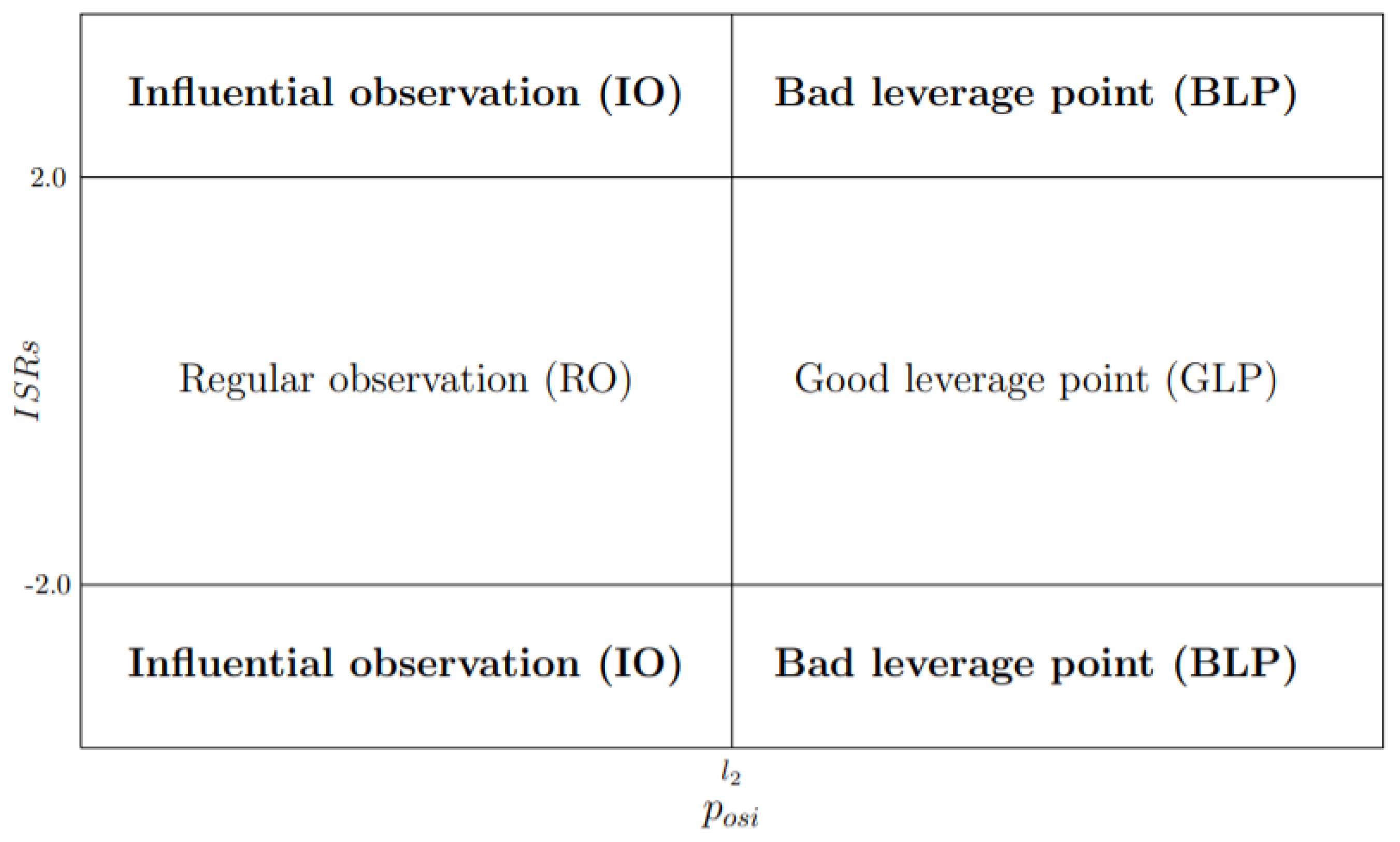
- (a)
- i
- observation is declared RO if and .
- ii
- observation is GLP if and .
- iii
- observation is BLP if and .
- iv
- observation is IO if and .
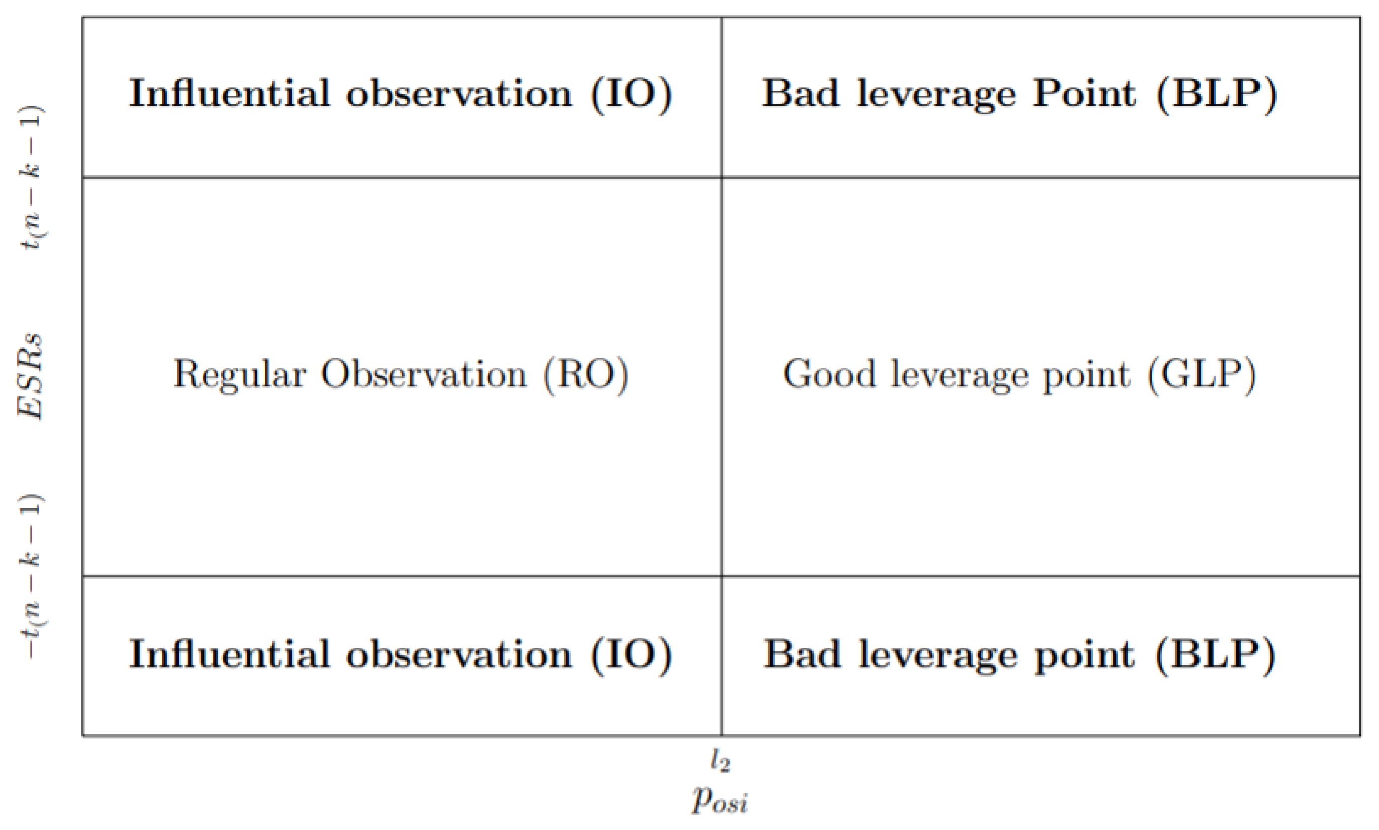
- (b)
- i
- observation is declared RO if and .
- ii
- observation is GL if and .
- iii
- observation is IO if and .
- iv
- observation is IO if and .
4. Results and Discussions
Simulated Data
5. Illustrative Examples
5.1. Example 1
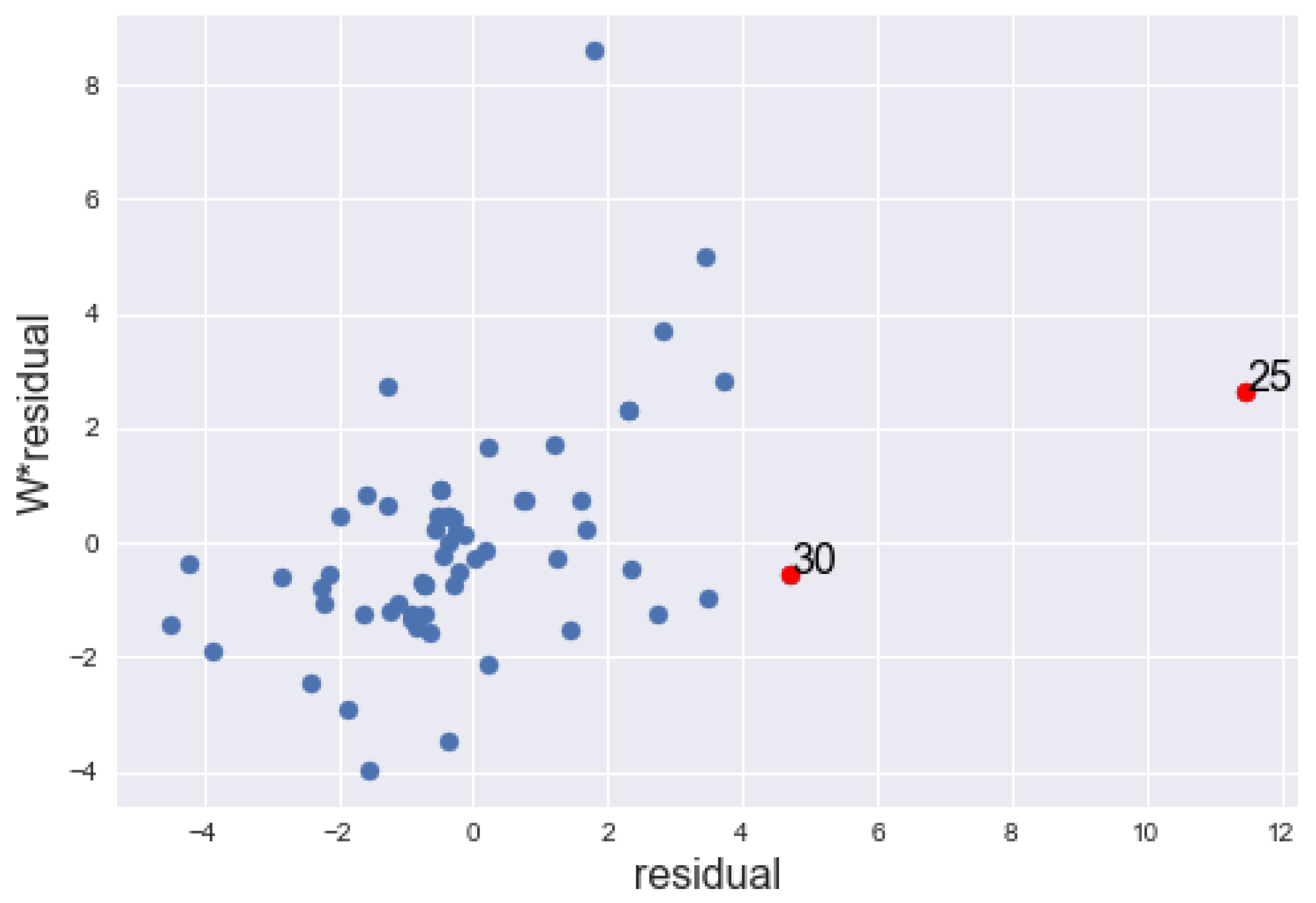
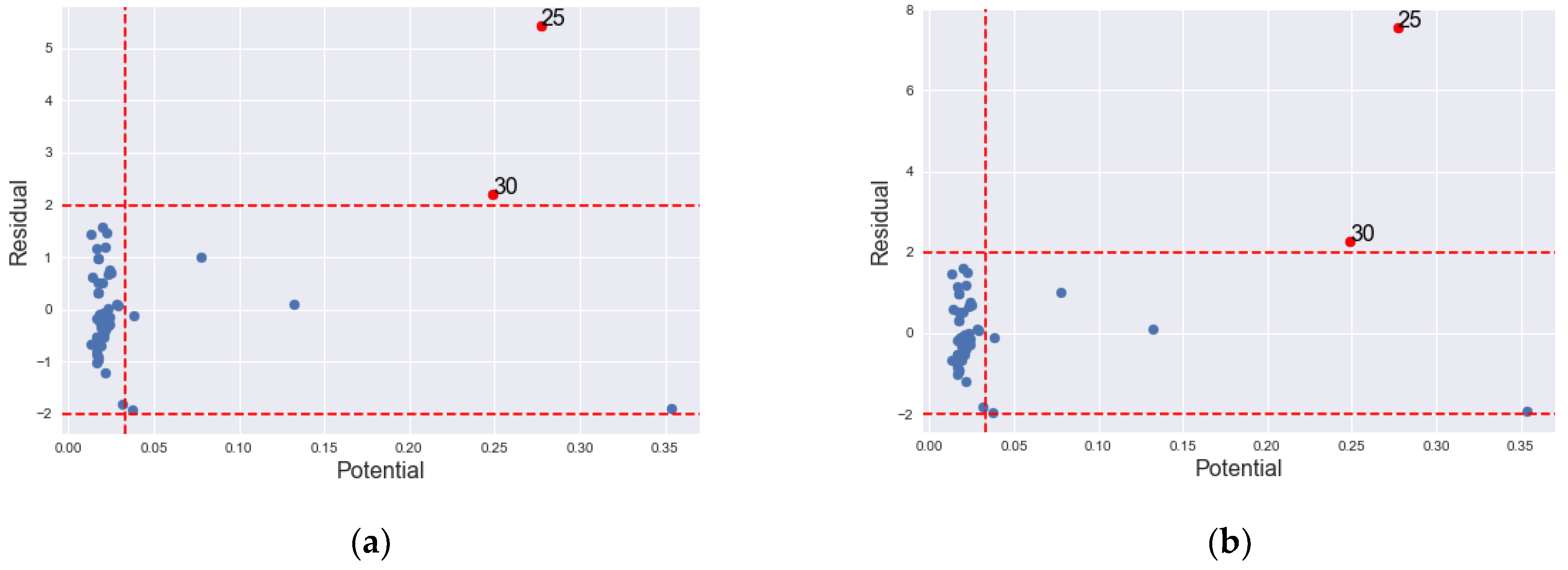
5.2. Example 2
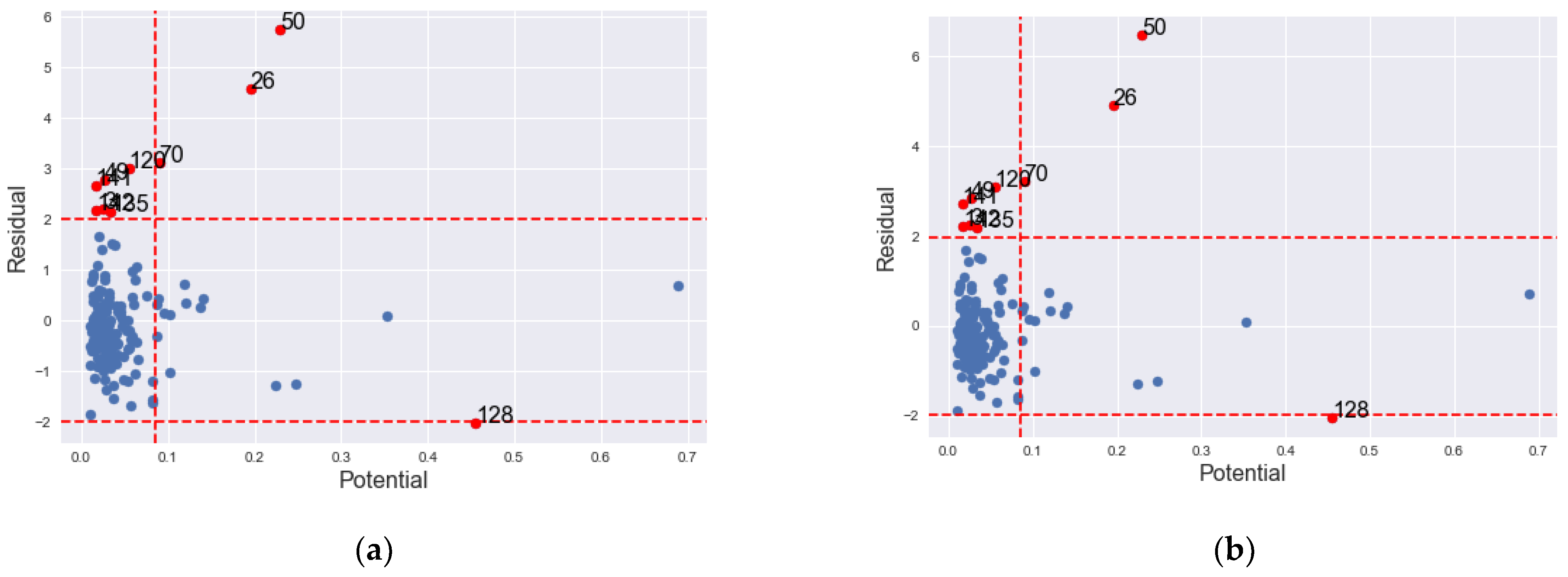
5.3. Example 3
6. Conclusions
Author Contributions
Funding
Data Availability Statement
Conflicts of Interest
References
- Belsley, D.A.; Kuh, E.; Welsch, R.E. Regression Diagnostics: Identifying Influential Data and Sources of Collinearity; John Wiley & Sons: New York, NY, USA, 1980; Volume 571. [Google Scholar]
- Rashid, A.M.; Midi, H.; Slwabi, W.D.; Arasan, J. An Efficient Estimation and Classification Methods for High Dimensional Data Using Robust Iteratively Reweighted SIMPLS Algorithm Based on Nu -Support Vector Regression. IEEE Access 2021, 9, 45955–45967. [Google Scholar] [CrossRef]
- Cook, R.D. Influential Observations in Linear Regression. J. Am. Stat. Assoc. 1977, 74, 169–174. [Google Scholar] [CrossRef]
- Hoaglin, D.C.; Welsch, R.E. The Hat Matrix in Regression and ANOVA. Am. Stat. 1978, 32, 17. [Google Scholar] [CrossRef]
- Andrews, D.F.; Pregibon, D. Finding the Outliers That Matter. J. R. Stat. Soc. Ser. B (Methodol.) 1978, 40, 85–93. [Google Scholar] [CrossRef]
- Hawkins, D.M. Identification of Outliers; Springer: Berlin/Heidelberg, Germany, 1980; Volume 11. [Google Scholar]
- Huber, P. Robust Statistics; John Wiley and Sons: New York, NY, USA, 1981. [Google Scholar]
- Cook, R.D.; Weisberg, S. Monographs on statistics and applied probability. In Residuals and Influence in Regression; Chapman and Hall: New York, NY, USA, 1982; ISBN 978-0-412-24280-9. [Google Scholar]
- Chatterjee, S.; Hadi, A.S. Sensitivity Analysis in Linear Regression; John Wiley & Sons: New York, NY, USA, 1988; Volume 327. [Google Scholar]
- Hadi, A.S. A New Measure of Overall Potential Influence in Linear Regression. Comput. Stat. Data Anal. 1992, 14, 1–27. [Google Scholar] [CrossRef]
- Habshah, M.; Norazan, M.R.; Rahmatullah Imon, A.H.M. The Performance of Diagnostic-Robust Generalized Potentials for the Identification of Multiple High Leverage Points in Linear Regression. J. Appl. Stat. 2009, 36, 507–520. [Google Scholar] [CrossRef]
- Meloun, M.; Militkỳ, J. Statistical Data Analysis: A Practical Guide; Woodhead Publishing Limited: Sawston, Cambridge, UK, 2011. [Google Scholar]
- Puterman, M.L. Leverage and Influence in Autocorrelated Regression Models. J. R. Stat. Soc. Ser. C (Appl. Stat.) 1988, 37, 76–86. [Google Scholar] [CrossRef]
- Schall, R.; Dunne, T.T. A Unified Approach to Outliers in the General Linear Model. Sankhyā Indian J. Stat. Ser. B 1988, 50, 157–167. [Google Scholar]
- Martin, R.J. Leverage, Influence and Residuals in Regression Models When Observations Are Correlated. Commun. Stat.-Theory Methods 1992, 21, 1183–1212. [Google Scholar] [CrossRef]
- Shi, L.; Chen, G. Influence Measures for General Linear Models with Correlated Errors. Am. Stat. 2009, 63, 40–42. [Google Scholar] [CrossRef]
- Cerioli, A.; Riani, M. Robust Transformations and Outlier Detection with Autocorrelated Data. In From Data and Information Analysis to Knowledge Engineering; Spiliopoulou, M., Kruse, R., Borgelt, C., Nürnberger, A., Gaul, W., Eds.; Studies in Classification, Data Analysis, and Knowledge Organization; Springer: Berlin/Heidelberg, Germany, 2006; pp. 262–269. ISBN 978-3-540-31313-7. [Google Scholar]
- Christensen, R.; Johnson, W.; Pearson, L.M. Prediction Diagnostics for Spatial Linear Models. Biometrika 1992, 79, 583–591. [Google Scholar] [CrossRef]
- Haining, R. Diagnostics for Regression Modeling in Spatial Econometrics*. J. Reg. Sci. 1994, 34, 325–341. [Google Scholar] [CrossRef]
- Haining, R.P.; Haining, R. Spatial Data Analysis: Theory and Practice; Cambridge University Press: Cambridge, UK, 2003. [Google Scholar]
- Dai, X.; Jin, L.; Shi, A.; Shi, L. Outlier Detection and Accommodation in General Spatial Models. Stat. Methods Appl. 2016, 25, 453–475. [Google Scholar] [CrossRef]
- Singh, A.K.; Lalitha, S. A Novel Spatial Outlier Detection Technique. Commun. Stat. -Theory Methods 2018, 47, 247–257. [Google Scholar] [CrossRef]
- Anselin, L. Some Robust Approaches to Testing and Estimation in Spatial Econometrics. Reg. Sci. Urban Econ. 1990, 20, 141–163. [Google Scholar] [CrossRef]
- Cerioli, A.; Riani, M. Robust Methods for the Analysis of Spatially Autocorrelated Data. Stat. Methods Appl. 2002, 11, 335–358. [Google Scholar] [CrossRef]
- Yildirim, V.; Mert Kantar, Y. Robust Estimation Approach for Spatial Error Model. J. Stat. Comput. Simul. 2020, 90, 1618–1638. [Google Scholar] [CrossRef]
- Kou, Y.; Lu, C.-T. Outlier Detection, Spatial. In Encyclopedia of GIS; Springer: Boston, MA, USA, 2008; pp. 1539–1546. [Google Scholar]
- Hadi, A.S.; Imon, A.H.M.R. Identification of Multiple Outliers in Spatial Data. Int. J. Stat. Sci. 2018, 16, 87–96. [Google Scholar]
- Hadi, A.S.; Simonoff, J.S. Procedures for the Identification of Multiple Outliers in Linear Models. J. Am. Stat. Assoc. 1993, 88, 1264–1272. [Google Scholar] [CrossRef]
- Aggarwal, C.C. Spatial Outlier Detection. In Outlier Analysis; Springer: New York, NY, USA, 2013; pp. 313–341. ISBN 978-1-4614-6395-5. [Google Scholar]
- Anselin, L. Local Indicators of Spatial Association—LISA. Geogr. Anal. 1995, 27, 93–115. [Google Scholar] [CrossRef]
- Politis, D.; Romano, J.; Wolf, M. Bootstrap Sampling Distributions. In Subsampling; Springer: New York, NY, USA, 1999; Available online: https://link.springer.com/chapter/10.1007/978-1-4612-1554-7_1 (accessed on 16 September 2021).
- Heagerty, P.J.; Lumley, T. Window Subsampling of Estimating Functions with Application to Regression Models. J. Am. Stat. Assoc. 2000, 95, 197–211. [Google Scholar] [CrossRef]
- Anselin, L. Exploratory Spatial Data Analysis and Geographic Information Systems. New Tools Spat. Anal. 1994, 17, 45–54. [Google Scholar]
- Cressie, N.A.C. Statistics for Spatial Data, Rev. ed.; Wiley series in probability and mathematical statistics; Wiley: New York, NY, USA, 1993; ISBN 978-0-471-00255-0. [Google Scholar]
- Anselin, L. Spatial Econometrics: Methods and Models; Studies in Operational Regional Science; Springer: Dordrecht, The Netherlands, 1988; Volume 4, ISBN 978-90-481-8311-1. [Google Scholar]
- LeSage, J.P. The Theory and Practice of Spatial Econometrics; University of Toledo: Toledo, OH, USA, 1999; Volume 28. [Google Scholar]
- Olver, P.J.; Shakiban, C.; Shakiban, C. Applied Linear Algebra; Springer: Berlin/Heidelberg, Germany, 2006; Volume 1. [Google Scholar]
- Horn, R.A.; Johnson, C.R. Matrix Analysis, 2nd ed.; Cambridge University Press: Cambridge, NY, USA, 2012; ISBN 978-0-521-83940-2. [Google Scholar]
- Liesen, J.; Mehrmann, V. Linear Algebra; Springer Undergraduate Mathematics Series; Springer International Publishing: Cham, Germany, 2015; ISBN 978-3-319-24344-3. [Google Scholar]
- Shekhar, S.; Lu, C.-T.; Zhang, P. A Unified Approach to Detecting Spatial Outliers. GeoInformatica 2003, 7, 139–166. [Google Scholar] [CrossRef]
- Billor, N.; Hadi, A.S.; Velleman, P.F. BACON: Blocked Adaptive Computationally Efficient Outlier Nominators. Comput. Stat. Data Anal. 2000, 34, 279–298. [Google Scholar] [CrossRef]
- Imon, A. Identifying Multiple High Leverage Points in Linear Regression. J. Stat. Stud. 2002, 3, 207–218. [Google Scholar]
- Rahmatullah Imon, A.H.M. Identifying Multiple Influential Observations in Linear Regression. J. Appl. Stat. 2005, 32, 929–946. [Google Scholar] [CrossRef]
- Midi, H.; Mohammed, A. The Identification of Good and Bad High Leverage Points in Multiple Linear Regression Model. Math. Methods Syst. Sci. Eng. 2015, 147–158. [Google Scholar]
- Bagheri, A.; Midi, H. Diagnostic Plot for the Identification of High Leverage Collinearity-Influential Observations. Sort: Stat. Oper. Res. Trans. 2015, 39, 51–70. [Google Scholar]
- Dowd, P. The variogram and kriging: Robust and resistant estimators. In Geostatistics for Natural Resources Characterization; Springer: Berlin/Heidelberg, Germany, 1984; pp. 91–106. [Google Scholar]

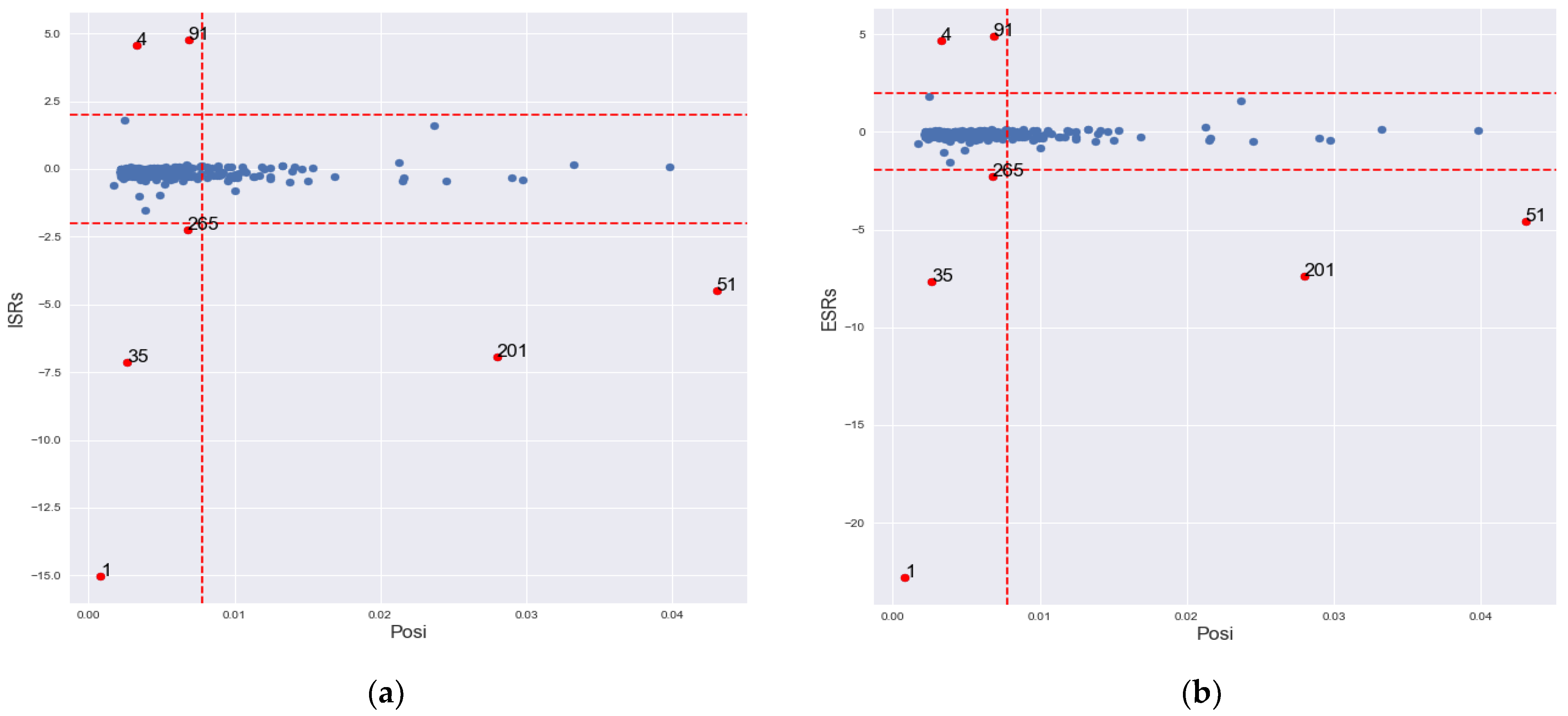
| Location | ISRs (2.00) | ESRs (1.97) | posi (0.0078) |
|---|---|---|---|
| 1 | 15.0378 | 22.8179 | 0.0008 |
| 4 | 4.5847 | 4.7046 | 0.0033 |
| 35 | −7.1434 | −7.6397 | 0.0026 |
| 51 | −4.4695 | −4.5801 | 0.0430 |
| 91 | 4.7613 | 4.8965 | 0.0068 |
| 201 | −6.9336 | −7.3840 | 0.0280 |
| 265 | −2.2644 | −2.2762 | 0.0068 |
| Method | Accurate Classification (%) | Swamping (%) | |
|---|---|---|---|
| 22.25 | 0.0 | ||
| 98.54 | 0.0 | ||
| 0.01 | 100.00 | 0.0 | |
| 39.45 | 0.0 | ||
| 99.71 | 81.41 | ||
| 20.64 | 0.0 | ||
| 98.36 | 0.0 | ||
| 0.1 | 100.00 | 0.0 | |
| 38.09 | 0.0 | ||
| 99.14 | 76.48 | ||
| 17.86 | 0.00 | ||
| 97.51 | 0.00 | ||
| 0.2 | 100.00 | 0.00 | |
| 37.23 | 0.00 | ||
| 97.34 | 69.25 | ||
| 16.36 | 0.00 | ||
| 96.57 | 0.00 | ||
| 0.3 | 100.00 | 0.00 | |
| 36.23 | 0.00 | ||
| 96.00 | 64.42 |
| S/N | Site | ISRs (2.00) | ESRs (2.00) | posi 0.0335 | CDsi | ISRs − Posi | ESRs − Posi | ||
|---|---|---|---|---|---|---|---|---|---|
| 1. | 3 | −1.8879 | −1.9301 | 0.3538 | no | No | No | no | Yes |
| 2. | 9 | 1.4810 | 1.4962 | 0.0223 | no | No | No | no | Yes |
| 3. | 22 | 1.0127 | 1.0129 | 0.0779 | no | No | No | no | Yes |
| 4. | 25 | 5.4292 | 7.5481 | 0.2773 | yes | Yes | Yes | yes | Yes |
| 5. | 26 | 1.4438 | 1.4573 | 0.1352 | no | No | No | no | Yes |
| 6. | 30 | 2.2054 | 2.2813 | 0.2489 | no | No | No | no | Yes |
| 7. | 40 | 1.5692 | 1.5890 | 0.0194 | no | No | No | no | Yes |
| 8. | 41 | 1.1974 | 1.2058 | 0.0218 | no | No | No | no | Yes |
| 9. | 42 | −1.9150 | −1.9598 | 0.0378 | no | No | No | no | Yes |
| 10. | 46 | 0.1003 | 0.0995 | 0.1319 | no | No | No | no | Yes |
| 11. | 55 | −1.2042 | −1.2089 | 0.0219 | no | No | No | no | Yes |
| 12. | 61 | −1.8011 | −1.8363 | 0.0319 | no | No | No | no | Yes |
| County | ISRs (2.00) | ESRs (1.98) | psi 0.0851 | CDsi | ISRs – Posi | ESRs – Posi | ||
|---|---|---|---|---|---|---|---|---|
| 3 | 2.2245 | 2.2539 | 0.0257 | no | no | no | no | Yes |
| 26 | 4.5733 | 4.9060 | 0.1956 | no | yes | yes | yes | Yes |
| 49 | 2.7685 | 2.8313 | 0.0265 | no | yes | Yes | no | Yes |
| 50 | 5.7504 | 6.4737 | 0.2298 | yes | yes | Yes | yes | Yes |
| 58 | 0.7090 | 0.7079 | 0.6893 | no | no | No | yes | Yes |
| 67 | 0.1018 | 0.1015 | 0.3524 | no | no | No | no | Yes |
| 70 | 3.1334 | 3.2285 | 0.0895 | no | yes | Yes | no | Yes |
| 98 | −1.8549 | −1.8699 | 0.0105 | no | no | No | no | Yes |
| 118 | −1.5657 | −1.5731 | 0.0827 | no | no | No | no | Yes |
| 120 | 3.0168 | 3.1006 | 0.0544 | no | yes | Yes | no | Yes |
| 128 | −2.0152 | −2.0359 | 0.4557 | no | yes | yes | no | Yes |
| 131 | −1.6718 | −1.6862 | 0.0565 | no | no | No | no | Yes |
| 134 | −1.6168 | −1.6253 | 0.0818 | no | no | No | no | Yes |
| 135 | 2.1674 | 2.1942 | 0.0338 | no | yes | Yes | no | Yes |
| 141 | 2.6726 | 2.7283 | 0.0163 | no | Yes | yes | no | Yes |
| 142 | 2.1805 | 2.2079 | 0.0174 | Yes | yes | no | no | Yes |
| 153 | −1.2693 | −1.2718 | 0.2234 | No | No | no | no | Yes |
| 155 | −1.2334 | −1.2359 | 0.2472 | No | No | no | no | Yes |
Publisher’s Note: MDPI stays neutral with regard to jurisdictional claims in published maps and institutional affiliations. |
© 2021 by the authors. Licensee MDPI, Basel, Switzerland. This article is an open access article distributed under the terms and conditions of the Creative Commons Attribution (CC BY) license (https://creativecommons.org/licenses/by/4.0/).
Share and Cite
Baba, A.M.; Midi, H.; Adam, M.B.; Abd Rahman, N.H. Detection of Influential Observations in Spatial Regression Model Based on Outliers and Bad Leverage Classification. Symmetry 2021, 13, 2030. https://doi.org/10.3390/sym13112030
Baba AM, Midi H, Adam MB, Abd Rahman NH. Detection of Influential Observations in Spatial Regression Model Based on Outliers and Bad Leverage Classification. Symmetry. 2021; 13(11):2030. https://doi.org/10.3390/sym13112030
Chicago/Turabian StyleBaba, Ali Mohammed, Habshah Midi, Mohd Bakri Adam, and Nur Haizum Abd Rahman. 2021. "Detection of Influential Observations in Spatial Regression Model Based on Outliers and Bad Leverage Classification" Symmetry 13, no. 11: 2030. https://doi.org/10.3390/sym13112030
APA StyleBaba, A. M., Midi, H., Adam, M. B., & Abd Rahman, N. H. (2021). Detection of Influential Observations in Spatial Regression Model Based on Outliers and Bad Leverage Classification. Symmetry, 13(11), 2030. https://doi.org/10.3390/sym13112030