Abstract
Quantum turbulence is characterized by many degrees of freedom interacting non-linearly to produce disordered states, both in space and in time. In this work, we investigate the decaying regime of quantum turbulence in a trapped Bose-Einstein condensate. We present an alternative way of exploring this phenomenon by defining and computing a characteristic length scale, which possesses relevant characteristics to study the establishment of the quantum turbulent regime. We reconstruct the three-dimensional momentum distributions with the inverse Abel transform, as we have done successfully in other works. We present our analysis with both the two- and three-dimensional momentum distributions, discussing their similarities and differences. We argue that the characteristic length allows us to intuitively visualize the time evolution of the turbulent state.
1. Introduction
Turbulence is a process that occurs in many types of fluids and a broad range of length scales, and it is characterized by chaotic changes in the flow velocity and pressure. The field of quantum turbulence (QT) investigates turbulence in quantum fluids, mainly liquid helium and trapped Bose-Einstein condensates (BECs) [1,2]. Many features of classical turbulence are not entirely explained, to the extent that Feynman deemed it the most important unsolved problem in classical physics [3]. Consequently, dealing with QT may seem a challenging task [3]. However, turbulence in quantum fluids might be more manageable than its classical equivalent because the vortex circulation is quantized in the former and continuous in the latter. Furthermore, from a technical point of view, the advances in cooling and tuning the interparticle interactions in trapped atomic BECs make them attractive candidates for investigating quantum turbulence and connecting it to related fields [4].
The first observation of turbulence in a trapped BEC, and its self-similar expansion, dates to 2009 [5]. Since then, considerable progress has been made in identifying and characterizing QT. A significant breakthrough in the area was the observation of a particle cascade, which appears as a power law in the momentum distribution [6,7],
where is a positive constant, and its value depends on the mechanism behind the generation of the turbulent state.
There are some intrinsic obstacles in determining the momentum range, where the power law is observed and its characteristic exponent. The range of momentum scales present in trapped BEC systems is small compared to superfluid helium, for example. The exponent of the power law depends on the mechanism behind the turbulence, and different theoretical models predict exponents to be close together. Unfortunately, experiments do not have the necessary precision to distinguish between them. Hence, strategies other than the power law identification have been employed to identify and characterize QT. Energy and particle fluxes have been used in simulations [8,9] and experiments [10,11] to overcome some of these difficulties. Since turbulence and disorder are intimately related, an approach based on the entropy of turbulent BECs has also been successfully applied [12] as an alternative method to investigate and characterize quantum turbulence.
A typical scale used to study turbulence in liquid helium is the vortex line density. Its time dependence provides evidence of the mechanism behind the turbulent regime [13]. In some He experiments, where visualization techniques are well-developed, the geometry and interactions of vortices can be directly observed [14]. In trapped BECs, where the range of length scales available is much smaller, the visualization techniques have not yet reached the same level of detail.
In this work, we employed a length scale associated with the momentum distribution to study the onset of turbulence and the turbulent state. It is inspired by the integral length scale, which is a quantity commonly used in classical turbulence. If we assume isotropic flow, then the integral length scale can be written in terms of the incompressible kinetic energy spectrum [13,15,16],
Casting Equation (2) in this form also illustrates that it is the length scale that contains most of the energy of the system.
It is known from numerical simulations that in some cases turbulence is mainly in the form of waves, and in sother cases mainly in the form of vortices, depending on the excitation protocol and boundary conditions of the system. Since moving vortices radiate waves and strong waves can create vortices, the relative proportion of waves and vortices depends on the particular experiment. In numerical simulations, one has access to the phase of the wave function [17]. Thus, the circulation can be computed to distinguish vortices from waves. Moreover, in the simulations, one can formally identify the compressible kinetic energy, which comes from waves, and the incompressible kinetic energy related to vortices. Unlike in the simulations, in the experiments, we cannot separate waves and vortices so easily.
However, with current experimental techniques, we can measure the momentum distribution independently of its origin: waves, vortices, or a combination of both. Hence, with Equation (2) in mind, we define the following length scale,
Intuitively, L is associated with the scale where most of the particles reside. In this work, we investigated the behavior of this quantity, and we showed that it is possible to use it to study a turbulent BEC.
Besides the difficulties mentioned above, there is also an experimental challenge when studying QT in trapped BECs. The momentum distribution of the cloud is obtained using a two-dimensional (2D) projection of the three-dimensional (3D) condensate. We employed the inverse Abel transform, an integral transform that connects the 2D projection of an axially or spherically symmetric function to its 3D value, to reconstruct the momentum distribution of the three-dimensional cloud. We showed that the results for the characteristic length scale are qualitatively the same if calculated using the two-dimensional projection. This indicates that it is possible to study some aspects of the turbulent states using the experimental data directly, without reconstructing the three-dimensional cloud.
This work is structured as follows. First, we provide the experimental details of how the BECs are produced and excited. Then, we present the momentum distributions in both two and three dimensions. These are used to compute the characteristic length scale and other quantities related to it. We discuss both the implications of our findings regarding the length scale and the projection of the cloud. In the Appendix A, we provide the Abel transforms of momentum distributions relevant to our system.
2. Experimental Procedure
The first step is the production of a Bose-Einstein condensate in equilibrium. A typical BEC contains rubidium-87 atoms in the hyperfine state , confined in a Quadrupole–Ioffe configuration (QUIC) magnetic trap of frequencies and . Hereafter, we adopted the convention of reporting the uncertainties as one standard deviation between parenthesis. Before any excitation is applied, the BEC in equilibrium has a condensate fraction of . The chemical potential at the center of the cloud is , and the healing length is = 0.15(2) m.
In Figure 1a, we present schematically the protocol we employed to drive the BEC out of equilibrium. Following the condensate production, an oscillating magnetic field is applied while it is still in the trap. The field is produced by a pair of coils, placed in an anti-Helmholtz configuration, with their axis tilted by a small angle of approximately 5 with respect to the axis of the trap. The excitation potential is given by , where is the coordinate in the rotated frame and = 42 m is the in-trap extent of the BEC along the x-axis of the trap. Since the perturbation is not aligned with the axes of the trap, the oscillations generate deformations, displacements, and rotations. Several excitation parameters can be varied, such as the amplitude A, total excitation time, and perturbation frequency. In this work, we performed the parametric excitation of fixed frequency , close to the radial trapping frequency, .
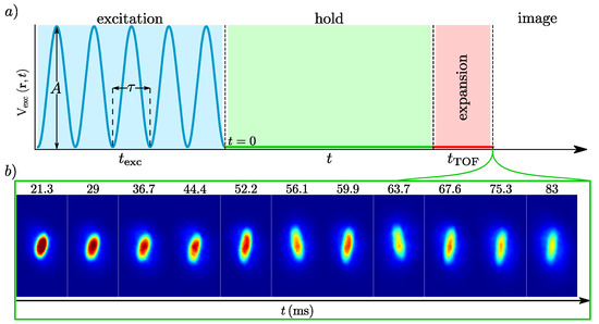
Figure 1.
(a) Schematic representation of the excitation protocol. The experiment begins with the production of an unperturbed BEC in the trap. Then, a sinusoidal potential of amplitude A and period is applied during . The system evolves during a time t, after which the trap is released, and an absorption image is taken after a time-of-flight . (b) Absorption images for an excitation amplitude of as a function of the holding time.
We increased the excitation amplitude until reaching a value where the momentum distribution corresponds to an out-of-equilibrium state, and we look for turbulent characteristics. The energy input to the condensate is related to both the total excitation time and the amplitude of the perturbation. Larger amplitudes need less time to reach similar conditions than it would take for smaller amplitudes. The range of amplitudes and excitation times to obtain a turbulent state was the topic of investigation in previous works [18]. In this work, we chose to apply the excitation protocol during a time , where . The amplitude A is varied, ranging from 0 (no perturbation) to .
After the excitation is turned off, we hold the cloud for a time t inside the trap, often called holding time, which is varied from 20 to 90 ms. During this time, the temporal evolution of the momentum distribution , which we are interested in, occurs. Next, we turn off the trap potential and measure using absorption images taken from the ballistic expansion of the cloud after a time of flight (ToF) of . In Figure 1b, we show typical absorption images corresponding to an excitation amplitude of for different holding times t.
For each excitation amplitude and holding time, we perform several realizations of the experiment and then average the results. In Figure 2, we show a typical two-dimensional momentum distribution obtained from the absorption images. The distance that an atom has traveled from the center of the cloud, after a time , is given by , where m is the mass of a rubidium-87 atom. Thus, in practice, the ToF technique corresponds to a Fourier transform of the spatial distribution, which yields the momentum distribution, . There are known shortcomings of the ToF technique, which do not significantly impact the measurement of our momentum distributions, mainly because the turbulent state is kinetically dominated [19]. For a more detailed discussion, the reader is referred to Reference [12] and references therein. This technique has been used successfully in the past to obtain the momentum distribution of turbulent trapped BECs [6,7].
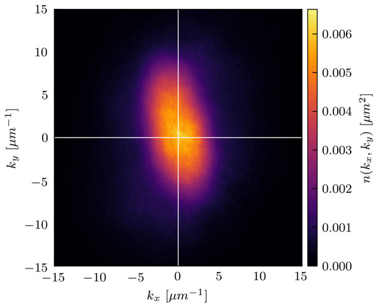
Figure 2.
Momentum distribution obtained from the absorption images of the cloud for an excitation of amplitude and .
3. Momentum Distributions
We performed angular averages on the momentum distributions obtained from the absorption images, such that the resulting profiles depend only on . The two-dimensional momentum distributions are normalized according to
As discussed above, an experimental challenge when studying momentum distributions of trapped BECs is that the absorption images correspond to a projection of the cloud. We overcome this difficulty by considering the symmetry of the trapped BEC in momentum space. The inverse Abel transform [20,21,22] has been successfully used in the literature [6,7] to obtain the 3D momentum distribution from its two-dimensional projection. It is an integral transform given by
We normalized the distributions according to
The signature of a particle cascade is a power law, . Equations (4) and (6), together with dimensional analysis, suggest that if we observe a power law both in the two-dimensional momentum distribution, , and in the three-dimensional one, , then their exponents differ by one, . To go beyond simple dimension analysis, in Appendix A, we derive this relation analytically for the case where a power law is present over the whole k-range. Although this toy-model is nonphysical, it sheds light on how we can reconstruct the three-dimensional momentum distribution based on symmetry arguments.
In our system, the low-momenta region of is dominated by the presence of the condensate, which corresponds to a Gaussian distribution. We show in Appendix A that the inverse Abel transform of a Gaussian function is also a Gaussian with the same width. This symmetry is extremely useful because we can work with the two-dimensional projections for quantities related to the Gaussian shape without the need for 3D reconstruction. This is the case of the temperature, which is related to the width of the Gaussian.
All the arguments presented above indicate that the power-law exponents in an ideal situation would be related through . However, the fact that we have the power-law behavior superimposed with the condensate at the low-momenta region of the momentum distribution alters this relation. Hence, we need to verify the exponents with the experimental data.
A power law is simply a line in a log–log plot of the momentum distribution as a function of k. We then look for a time window when, in a certain k-range, is proportional to , the particle cascade characteristic of a turbulent cloud. We performed the experiment described in Section 2 employing six different excitation amplitudes. For only the three highest ones, A = 1.8, 2.0, and 2.2 , we observed the appearance of a power-law, around 35 ms and in the region 10 m 15 m. We found the exponents and , which lead to . It is interesting to see that even in our finite-sized non-homogeneous system inside an anisotropic trap, we still have close to one.
In Figure 3, we present the time evolution of both the two- and three-dimensional momentum distributions for an excitation amplitude of A = 1.8 (which is qualitatively the same for A = 2.0 and 2.2 ). As we wait after the external excitation has been turned off, the distribution evolves, promoting the population from low to high momentum values, as can be seen in Figure 3.
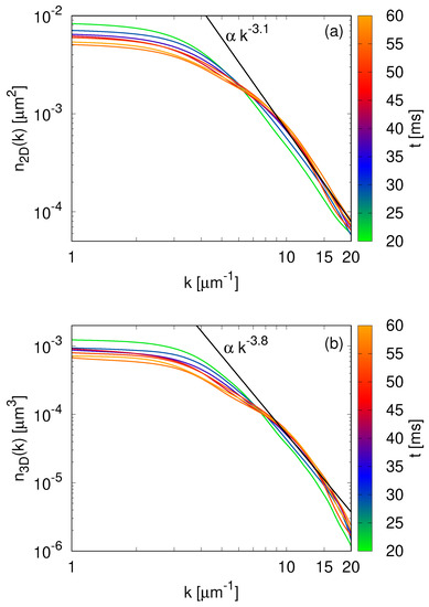
Figure 3.
Time evolution of the momentum distributions for an excitation amplitude of A = 1.8 . We present the results obtained with both (a) the angular average of the absorption image and (b) the three-dimensional reconstruction of the cloud using the inverse Abel transform. In both plots, we include the curve corresponding to the power-law behavior characteristic of the turbulent states as a guide to the eye.
Some words regarding the values of the exponents we found are in order. To the best of our knowledge, there is no theoretical work that describes all aspects of the experiments we performed, mainly for two reasons. First, our condensate is produced in an anisotropic trap. From the theoretical perspective, it is much easier to implement periodic boundary conditions and describe, or simulate, bulk systems. Second, the route we take is the inverse of most experiments. We begin with a BEC in equilibrium and then excite it, while, for example, quench experiments usually start with a thermal gas and produce a condensate [23,24]. However, after these considerations, we can compare the momentum distributions and exponent we obtained with other works that share similarities with our experiment.
One of the first predictions for the time evolution of the momentum distribution describing Bose-Einstein condensation in a far-from-equilibrium system is given in Reference [25]. The authors find a plateau in the lower momenta region and a power law at higher momenta, akin to what we observe in our experiments; see Figure 3. Since then, much progress has been made in characterizing turbulent flows in BECs. The advances and state of the art concerning this topic can be found in Reference [26], for example. Here, we will discuss two references that capture the essential physical aspects of our experiment.
The authors of [27] address the topic of turbulence in ultracold Bose gases under the light of the so-called non-thermal fixed points [28]. They consider a variety of scenarios and analyze each region of the momentum distributions. For strong turbulence and a freely (without external energy input or dissipation) decaying initial state, scaling arguments lead to prediction, which was confirmed by accompanying numerical simulations. We did not expect quantitative agreement with their results, since we have dissipation in our system, and there are no indications that we are in the strong turbulent regime. Nonetheless, this is one of the few references that address the decay of turbulence.
Another interesting study that allows comparison, to some extent, to our work is presented in Reference [29]. The authors performed numerical simulations employing the forced-dissipated Gross–Pitaevskii equation to study Bose-Einstein condensation under non-equilibrium conditions. They observed that the momentum distribution for the late time dynamics, that is, after the kinetic stage is over, displays an approximately constant value at low-momenta, in accordance with our findings, and a power law in a higher momentum region with the exponent (for some values of the nonlinear term). This value is relatively close to what we observed in this work, . We should remark that the boundary conditions in their simulations and our experiments are different and that we are exciting a BEC while they are looking at the inverse process. However, the agreement warrants further investigations.
4. The Characteristic Length Scale
We computed the characteristic length scale given by Equation (3) using the experimental data available,
where ∼0.05 m and ∼30 m are the smallest and largest wave vectors we can measure, respectively. It is worth noting that although our definition relies on , the singular behavior when will never be reached. The lower limit of the integrals, , is inversely proportional to the largest length scale of the system, which can be large concerning other scales, but always finite.
Using the momentum distributions obtained with different excitation amplitudes and holding times, we can study the time evolution of the BEC, ranging from a slightly perturbed cloud up to a turbulent state. In Figure 4, we present our results for the characteristic length scale computed with both the two-dimensional projection of the cloud and its three-dimensional reconstruction. Although they differ quantitatively, their qualitative behavior is remarkably the same.
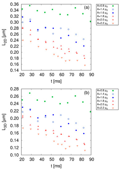
Figure 4.
Time evolution of the characteristic length scale for different excitation amplitudes computed with (a) the two-dimensional projection of the cloud and (b) its three-dimensional reconstruction using the inverse Abel transform. Although the values computed with two-dimensional profiles are higher, their qualitative behavior is the same.
The value can be interpreted as the evolution of the length scale where most of the particles are located. If we think of as being a weight in Equation (3), then is related to the inverse of the momentum value for which is peaked. Nucleation of excitations occurs during the excitation, whether in the form of vortices or waves. Then the interaction of these excitations takes place, leading to different stages of deviation from equilibrium.
For small excitation amplitudes, 0.8 , the system is only slightly disturbed and removed from equilibrium, but it does not have enough energy to reach what is considered a disordered state. In this case, it evolves differently from the others, and the value of L is approximately constant with time.
For intermediate perturbations, 1.4 and 1.6 , there is a separation between these results and the smallest amplitude, besides a clear dependence with time. For these excitation amplitudes, we are in a regime best characterized as the onset of turbulence. The characteristic length scale decreases on time, indicating the particle transfer to higher-momenta, but slower than the higher excitation amplitudes.
In this work and previous investigations [12], we identified the highest excitation amplitudes with turbulent clouds, 1.8, 2.0, and 2.2 . The value of at the end of the processes seems to depend on the amplitude and, more importantly, if we deal with a moderate perturbation, the onset of turbulence, or a state with turbulent characteristics. It is interesting to observe that the turbulent states quickly reach lengths comparable to the healing length ( = 0.15(2) m), where dissipation processes are expected to occur.
The behavior of the characteristic length scale can be described by an exponential decay,
where is the extrapolation of the characteristic length scale to the instant when the excitation was introduced, and is its characteristic time.
In Figure 5, we present the values of and fitted to the functional form of Equation (8) for different excitation amplitudes. We did not include the results for 0.8 , since we obtain a value of 750 ms, of the same order as the lifetime of the condensate.
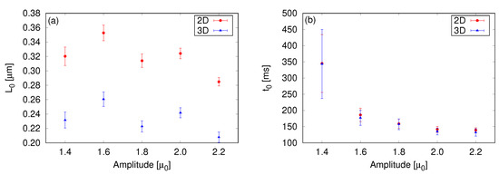
Figure 5.
(a) Extrapolation of the characteristic length scale to the instant when the excitation is turned on, , and (b) the characteristic time of the particle transfer, , as a function of the excitation amplitude. The results were obtained fitting the data to the functional form of Equation (8). Although the analysis employing two- or three-dimensional momentum distributions produces different values of , both approaches yield the same values for the characteristic time.
Figure 5a shows that the length containing most particles of the system is approximately the same with respect to the excitation amplitudes. However, if we perform the analysis employing the two- or three-dimensional momentum distributions, we arrive at different values for . A possible reason for this is that the inverse Abel transform slightly shifts the profiles toward higher-momena—see Figure 3—which then implies a smaller value of .
In Figure 5b, we present the characteristic time that the particle transfer takes as a function of the excitation amplitude. It is observed that decreases with amplitude, as expected, since larger amplitudes lead to a faster formation of excitations and, therefore, speed up the decay. It is possible to see that the results obtained in 2D and 3D are in remarkable agreement. This opens the possibility of studying dynamical processes in 2D without the need to reconstruct the three-dimensional cloud, depending on the quantity of interest.
5. Discussion and Final Remarks
In this work, we defined and computed a characteristic length scale related to the momentum distribution of a trapped BEC, which allowed us to identify distinct out-of-equilibrium stages: a slightly perturbed cloud, the onset of turbulence, and the turbulent state. This quantity complements the formal analysis of identifying a power-law in the momentum distribution as a hallmark of turbulence.
We also focused our efforts on calculating this characteristic length scale using both two- and three-dimensional momentum distributions. The former is obtained straightforwardly from the experimental data, and the latter is reconstructed based on the symmetry of the cloud. From a technical point of view, it is preferable to work only with the two-dimensional distributions, since no assumptions about the symmetry of the cloud have to be made. Although the length scales are affected by the inverse Abel transform, which shifts the momentum distributions to higher momenta, the qualitative behavior calculated in 2D and 3D is remarkably similar. The excellent agreement in the characteristic time of the particle transfer indicates that the two-dimensional analysis may be appropriate to investigate dynamical aspects of these systems.
One important remark is that isotropy is assumed through Equation (3) only for the kinetically dominated regions in Fourier space. Such an assumption can be made even for inhomogeneous cigar-shaped clouds. This is because such large-scale inhomogeneities affect only regions in Fourier space up to the order of , where is the smaller linear size of the cigar-shaped cloud. In a previous work [11], we studied the impact of anisotropy in the energy transfer during the evolution of turbulence in a trapped BEC. Like the integral length scale, the energy flux can also be computed from the kinetic energy spectrum. We found that the turbulent state can be identified and characterized in terms of the energy flux regardless of whether we employ the whole cloud or just a region close to the major axis of the expanded cloud. We should note that the axial trapping frequencies of this work and of Reference [11] are very close; however, in this work, we employ a radial trapping frequency that is ≈0.7 smaller than the one used in Reference [11]. Thus, the BECs in this work are much less elongated and closer to a spherical shape than the ones in Reference [11]. Therefore the range of validity for Equation (3) is even larger than in previous works.
In future works, we intend to vary the excitation protocol to investigate the changes in the characteristic length. Since there is a compromise between the excitation amplitude and time [18], it may prove insightful to investigate situations where the same amount of energy is introduced in the system but varying the time it takes to be injected from very slow inputs up to abrupt changes.
Author Contributions
Conceptualization, F.E.A.d.S. and V.S.B.; methodology, L.M.; software, L.M.; validation, L.M., A.D.G.-O. and M.A.M.-A.; formal analysis, L.M.; investigation, L.M., A.D.G.-O. and M.A.M.-A.; resources, V.S.B.; data curation, L.M., A.D.G.-O. and M.A.M.-A.; writing—original draft preparation, L.M.; writing—review and editing, F.E.A.d.S. and V.S.B.; visualization, L.M.; supervision, V.S.B.; project administration, L.M.; funding acquisition, V.S.B. All authors have read and agreed to the published version of the manuscript.
Funding
This work was supported by the São Paulo Research Foundation (FAPESP) under the grants 2013/07276-1, 2014/50857-8, and 2018/09191-7, and by the National Council for Scientific and Technological Development (CNPq) under the grant 465360/2014-9. FEAS thanks CNPq (Conselho Nacional de Desenvolvimento Científico e Tecnológico, National Council for Scientific and Technological Development) for support through Bolsa de produtividade em Pesquisa Grant No. 305586/2017-3.
Institutional Review Board Statement
Not applicable.
Informed Consent Statement
Not applicable.
Data Availability Statement
The data presented in this study are available on request from the corresponding author.
Acknowledgments
We thank L. Galantucci and C. Barenghi for the useful discussions.
Conflicts of Interest
The authors declare no conflict of interest.
Abbreviations
The following abbreviations are used in this manuscript:
| QT | Quantum turbulence |
| BEC | Bose-Einstein condensate |
| QUIC | Quadrupole–Ioffe configuration |
| ToF | Time-of-flight |
Appendix A. The Abel Transform
We used the inverse Abel transform to reconstruct a three-dimensional momentum distribution from its two-dimensional projection in the main text. It is insightful to take the inverse route to see what the two-dimensional projection is of a known three-dimensional . In this appendix, we considered two relevant cases for our physical system that possess analytical solutions.
The Abel transform is given by
The first case we considered is a Gaussian normalized according to Equation (6),
Using Equation (A1), the normalized two-dimensional projection is
Hence, the Abel transform of a Gaussian is a Gaussian of the same width. This is very convenient in the case of the temperature of the cloud, for example, since it is estimated through the width of the Gaussian profile of the momentum distribution.
The second case we considered is a power-law with exponent ,
with A constant. The standard normalization procedure, Equation (6), is going to fail because this momentum distribution is not valid in the entire domain. In reality, the power-law would be observed over a certain k-range, with . However, this simplified example will have an interesting result as we will see. The Abel transformation yields
where is the gamma function, is another constant, and . The conclusion is that the bidimensional projection of a power-law with an exponent of in three dimensions is also a power-law, but with the exponent increased by one.
Clearly, the momentum distributions we presented in the main text cannot be fully described by these two simple examples. However, they provide indications of the expected behavior of the projection procedure.
References
- Vinen, W.F.; Niemela, J.J. Quantum Turbulence. J. Low Temp. Phys. 2002, 128, 167–231. [Google Scholar] [CrossRef]
- Barenghi, C.F.; Skrbek, L.; Sreenivasan, K.R. Introduction to quantum turbulence. Proc. Natl. Acad. Sci. USA 2014, 111, 4647–4652. [Google Scholar] [CrossRef] [PubMed] [Green Version]
- Madeira, L.; Caracanhas, M.; dos Santos, F.; Bagnato, V. Quantum Turbulence in Quantum Gases. Annu. Rev. Condens. Matter Phys. 2020, 11, 37–56. [Google Scholar] [CrossRef]
- Dalfovo, F.; Giorgini, S.; Pitaevskii, L.P.; Stringari, S. Theory of Bose-Einstein condensation in trapped gases. Rev. Mod. Phys. 1999, 71, 463–512. [Google Scholar] [CrossRef] [Green Version]
- Henn, E.A.L.; Seman, J.A.; Roati, G.; Magalhães, K.M.F.; Bagnato, V.S. Emergence of Turbulence in an Oscillating Bose-Einstein Condensate. Phys. Rev. Lett. 2009, 103, 045301. [Google Scholar] [CrossRef]
- Thompson, K.J.; Bagnato, G.G.; Telles, G.D.; Caracanhas, M.A.; dos Santos, F.E.A.; Bagnato, V.S. Evidence of power law behavior in the momentum distribution of a turbulent trapped Bose-Einstein condensate. Laser Phys. Lett. 2014, 11, 015501. [Google Scholar] [CrossRef]
- Navon, N.; Gaunt, A.L.; Smith, R.P.; Hadzibabic, Z. Emergence of a turbulent cascade in a quantum gas. Nature 2016, 539, 72–75. [Google Scholar] [CrossRef] [Green Version]
- Baggaley, A.W.; Barenghi, C.F.; Sergeev, Y.A. Three-dimensional inverse energy transfer induced by vortex reconnections. Phys. Rev. E-Stat. Nonlinear Soft Matter Phys. 2014, 89, 013002. [Google Scholar] [CrossRef] [PubMed] [Green Version]
- Marino, Á.V.M.; Madeira, L.; Cidrim, A.; dos Santos, F.E.A.; Bagnato, V.S. Momentum distribution of Vinen turbulence in trapped atomic Bose-Einstein condensates. Eur. Phys. J. Spec. Top. 2021, 230, 809–812. [Google Scholar] [CrossRef]
- Navon, N.; Eigen, C.; Zhang, J.; Lopes, R.; Gaunt, A.L.; Fujimoto, K.; Tsubota, M.; Smith, R.P.; Hadzibabic, Z. Synthetic dissipation and cascade fluxes in a turbulent quantum gas. Science 2019, 366, 382–385. [Google Scholar] [CrossRef] [Green Version]
- Daniel García-Orozco, A.; Madeira, L.; Galantucci, L.; Barenghi, C.F.; Bagnato, V.S. Intra-scales energy transfer during the evolution of turbulence in a trapped Bose-Einstein condensate. EPL Europhys. Lett. 2020, 130, 46001. [Google Scholar] [CrossRef]
- Madeira, L.; García-Orozco, A.D.; dos Santos, F.E.A.; Bagnato, V.S. Entropy of a Turbulent Bose-Einstein Condensate. Entropy 2020, 22, 956. [Google Scholar] [CrossRef] [PubMed]
- Stagg, G.W.; Parker, N.G.; Barenghi, C.F. Ultraquantum turbulence in a quenched homogeneous Bose gas. Phys. Rev. A 2016, 94, 053632. [Google Scholar] [CrossRef] [Green Version]
- Bewley, G.P.; Lathrop, D.P.; Sreenivasan, K.R. Superfluid helium: Visualization of quantized vortices. Nature 2006, 441, 588. [Google Scholar] [CrossRef] [PubMed]
- Batchelor, G.K.; Press, C.U. The Theory of Homogeneous Turbulence; Cambridge Science Classics; Cambridge University Press: Cambridge, UK, 1953. [Google Scholar]
- WANG, H.; GEORGE, W.K. The integral scale in homogeneous isotropic turbulence. J. Fluid Mech. 2002, 459, 429–443. [Google Scholar] [CrossRef] [Green Version]
- Tsubota, M.; Fujimoto, K.; Yui, S. Numerical Studies of Quantum Turbulence. J. Low Temp. Phys. 2017, 188, 119–189. [Google Scholar] [CrossRef] [Green Version]
- Seman, J.A.; Henn, E.A.; Shiozaki, R.F.; Roati, G.; Poveda-Cuevas, F.J.; Magalhães, K.M.; Yukalov, V.I.; Tsubota, M.; Kobayashi, M.; Kasamatsu, K.; et al. Route to turbulence in a trapped Bose-Einstein condensate. Laser Phys. Lett. 2011, 8, 691–696. [Google Scholar] [CrossRef] [Green Version]
- Pitaevskii, L.; Stringari, S. Bose-Einstein Condensation and Superfluidity; Oxford University Press: Oxford, UK, 2016. [Google Scholar] [CrossRef]
- Bracewell, R.N.; Bracewell, R.N. The Fourier Transform and Its Applications; McGraw-Hill Series in Electrical Engineering; McGraw-Hill: New York, NY, USA, 1986. [Google Scholar]
- Polyanin, P.; Manzhirov, A.V. Handbook of Integral Equations, 2nd ed.; Handbooks of Mathematical Equations; CRC Press: Boca Raton, FL, USA, 2008. [Google Scholar]
- Hickstein, D.D.; Gibson, S.T.; Yurchak, R.; Das, D.D.; Ryazanov, M. A direct comparison of high-speed methods for the numerical Abel transform. Rev. Sci. Instrum. 2019, 90, 065115. [Google Scholar] [CrossRef]
- Proukakis, N.P.; Snoke, D.W.; Littlewood, P.B. (Eds.) Universal Themes of Bose-Einstein Condensation; Cambridge University Press: Cambridge, UK, 2017. [Google Scholar] [CrossRef]
- Glidden, J.A.P.; Eigen, C.; Dogra, L.H.; Hilker, T.A.; Smith, R.P.; Hadzibabic, Z. Bidirectional dynamic scaling in an isolated Bose gas far from equilibrium. Nat. Phys. 2021, 17, 457–461. [Google Scholar] [CrossRef]
- Semikoz, D.V.; Tkachev, I.I. Kinetics of Bose Condensation. Phys. Rev. Lett. 1995, 74, 3093–3097. [Google Scholar] [CrossRef] [Green Version]
- Semisalov, B.; Grebenev, V.; Medvedev, S.; Nazarenko, S. Numerical analysis of a self-similar turbulent flow in Bose-Einstein condensates. Commun. Nonlinear Sci. Numer. Simul. 2021, 102, 105903. [Google Scholar] [CrossRef]
- Nowak, B.; Schole, J.; Sexty, D.; Gasenzer, T. Nonthermal fixed points, vortex statistics, and superfluid turbulence in an ultracold Bose gas. Phys. Rev. A 2012, 85, 043627. [Google Scholar] [CrossRef] [Green Version]
- Schmied, C.M.; Mikheev, A.N.; Gasenzer, T. Non-thermal fixed points: Universal dynamics far from equilibrium. Int. J. Mod. Phys. A 2019, 34, 1941006. [Google Scholar] [CrossRef] [Green Version]
- Shukla, V.; Nazarenko, S. Non-equilibrium Bose-Einstein Condensation. arXiv 2021, arXiv:2105.07274. [Google Scholar]
Publisher’s Note: MDPI stays neutral with regard to jurisdictional claims in published maps and institutional affiliations. |
© 2021 by the authors. Licensee MDPI, Basel, Switzerland. This article is an open access article distributed under the terms and conditions of the Creative Commons Attribution (CC BY) license (https://creativecommons.org/licenses/by/4.0/).