Time-Dependent Conformal Transformations and the Propagator for Quadratic Systems ^†

Abstract

The method proposed by Inomata and his collaborators allows us to transform a damped Caldirola–Kanai oscillator with a time-dependent frequency to one with a constant frequency and no friction by redefining the time variable, obtained by solving an Ermakov–Milne–Pinney equation. Their mapping “Eisenhart–Duval” lifts as a conformal transformation between two appropriate Bargmann spaces. The quantum propagator is calculated also by bringing the quadratic system to free form by another time-dependent Bargmann-conformal transformation, which generalizes the one introduced before by Niederer and is related to the mapping proposed by Arnold. Our approach allows us to extend the Maslov phase correction to an arbitrary time-dependent frequency. The method is illustrated by the Mathieu profile.

1. Introduction

A nonrelativistic quantum particle with unit mass in $d+1$ spacetime dimensions with coordinates $x,t$ is given by the natural Lagrangian $L=\frac{1}{2}{\dot{x}}^2-V(x,t)$. The wave function is expressed in terms of the propagator,

$$\psi (x^{″},t^{″})=\int K(x^{″},t^{″}|x^{\prime },t^{\prime })\psi (x^{\prime },t^{\prime })d{x}^{\prime }$$

(1)

which, following Feynman’s intuitive proposal [1], is obtained as,

$$K(x^{″},t^{″}|x^{\prime },t^{\prime })=\int exp\left[\frac{i}{\hslash }\mathcal{A}\left(\gamma \right)\right]\mathcal{D}◯,$$

(2)

where the (symbolic) integration is over all paths $\gamma \left(t\right)= \left(x\left(t\right),t\right)$ that link the spacetime point $(x^{\prime },t^{\prime })$ to $(x^{″},t^{″})$ and where:

$$\mathcal{A}\left(\gamma \right)={\int }_{t^{\prime }}^{t^{″}}L\left(\gamma \left(t\right),\dot{\gamma }\left(t\right),t\right)dt$$

(3)

is the classical action calculated along $\gamma \left(t\right)$ [1,2,3].

The rigorous definition and calculation of (2) are beyond our scope here. However, the semiclassical approximation leads to the van Vleck–Pauli formula [2,3,4,5],

$$K(x^{″},t^{″}|x^{\prime },t^{\prime })={\left[\frac{i}{2\pi \hslash }\frac{{\partial }^2\overline{\mathcal{A}}}{\partial x^{\prime }\partial x^{″}}\right]}^{1/2}exp\left[\frac{i}{\hslash }\overline{\mathcal{A}}(x^{″},t^{″}|x^{\prime },t^{\prime })\right],$$

(4)

where ${\displaystyle \overline{\mathcal{A}}(x^{″},t^{″}|x^{\prime },t^{\prime })={\int }_{t^{\prime }}^{t^{″}}L(\overline{\gamma }\left(t\right),\dot{\overline{\gamma }}\left(t\right),t)dt}$ is the classical action calculated along the (supposedly unique (This condition is satisfied away from caustics [2,3,6]. Moreover, (5) and (8) are valid only for $0<T^{″}-T^{\prime }$ and for $0<t^{″}-t^{\prime }<\pi$, respectively, as discussed in Section 4.)) classical path $\overline{\gamma }\left(\tau \right)$ from $(x^{\prime },t^{\prime })$ and $(x^{″},t^{″})$. This expression involves data of the classical motion only. We note here also the van Vleck determinant $\frac{{\partial }^2\overline{\mathcal{A}}}{\partial x^{\prime }\partial x^{″}}$ in the prefactor [4,5].

Equation (4) is exact for a quadratic-in-the-position potentials in $1+1$ dimension $V(x,t)=\frac{1}{2}{\omega }^2\left(t\right)x^2$ that we consider henceforth.

For $\omega \equiv 0$, i.e., for a free nonrelativistic particle of unit mass in 1 + 1 dimensions with coordinates X and T, the result is [1,2,3],

$$K_{free}(X^{″},T^{″}|X^{\prime },T^{\prime })={\left[\frac{1}{2\pi i\hslash (T^{″}-T^{\prime })}\right]}^{1/2}exp\left\{\frac{i}{\hslash }\frac{{(X^{″}-X^{\prime })}^2}{2(T^{\prime \prime }-T^{\prime })}\right\}.$$

(5)

A harmonic oscillator with dissipation is in turn described by the Caldirola–Kanai (CK) Lagrangian and the equation of motion, respectively [7,8]. For constant damping and a harmonic frequency, we have,

$$\begin{array}{ccc}\hfill & & L_{CK}=\frac{1}{2}{e}^{{\lambda }_{0}t}\left({\left(\frac{dx}{dt}\right)}^2-{\omega }_0^2{x}^2\right),\hfill \end{array}$$

(6)

$$\begin{array}{ccc}\hfill & & \frac{d^{2}x}{d{t}^2}+{\lambda }_0\frac{dx}{dt}+{\omega }_0^{2}x=0\hfill \end{array}$$

(7)

with ${\lambda }_0=\mathrm{const}.>0$ and ${\omega }_0=\mathrm{const}.$. A lengthy calculation then yields the exact propagator [2,3,9,10,11]:

$$\begin{array}{ccc}\hfill & & K_{CK}(x^{″},t^{″}|x^{\prime },t^{\prime })={\left[\frac{{\mathsf{\Omega }}_0{e}^{\frac{{\lambda }_0}{2}(t^{″}+t^{\prime })}}{2\pi i\hslash sin\left[{\mathsf{\Omega }}_0(t^{″}-t^{\prime })\right]}\right]}^{\frac{1}{2}}\times \hfill \\ \hfill & & exp\left\{\frac{i{\mathsf{\Omega }}_0}{2\hslash sin\left[{\mathsf{\Omega }}_0(t^{″}-t^{\prime })\right]}\left[({x″}^2{e}^{{\lambda }_0{t}^{″}}+{x\prime }^2{e}^{{\lambda }_0{t}^{\prime }})cos\left[{\mathsf{\Omega }}_0(t^{″}-t^{\prime })\right]-2x^{″}{x}^{\prime }{e}^{{\lambda }_0\frac{t^{″}+t^{\prime }}{2}}\right]\right\},\hfill \end{array}$$

(8)

$$\begin{array}{ccc}\hfill & & {\mathsf{\Omega }}_0^2={\omega }_0^2-\frac{1}{4}{\lambda }_0^2,\hfill \end{array}$$

(9)

where an irrelevant phase factor was dropped.

Inomata and his collaborators [12,13,14,15] generalized (9) to a time-dependent frequency by redefining time, $t\to \tau$, which allowed them to transform the time-dependent problem to one with a constant frequency (see Section 2). Then, they followed by what they called a “time-dependent conformal transformation” $(x,t)\to (X,T)$ such that:

$$x=f\left(T\right)X\left(T\right)exp\left[\frac{1}{2}{\lambda }_{0}T\right],t=g\left(T\right),\mathrm{where}{f}^2\left(T\right)=\frac{dg}{dT},$$

(10)

which allowed them to derive the propagator from the free expression (5). When spelled out, (10) boils down to a generalized version, (22), of the correspondence found by Niederer [16].

It is legitimate to wonder: in what sense are these transformations “conformal” ? In Section 3, we explain that, in fact, both mappings can be interpreted in the Eisenhart–Duval (E-D) framework as conformal transformations between two appropriate Bargmann spaces [17,18,19,20,21]. Moreover, the change of variables $x,t\to X,T$ is a special case of the one put forward by Arnold [22,23] and is shown to be convenient to study time-dependent systems explicitly.

A bonus is the extension to the arbitrary time-dependent frequency $\omega \left(t\right)$ of the Maslov phase correction [2,4,5,6,19,24,25,26,27,28] even when no explicit solutions are available (see Section 4).

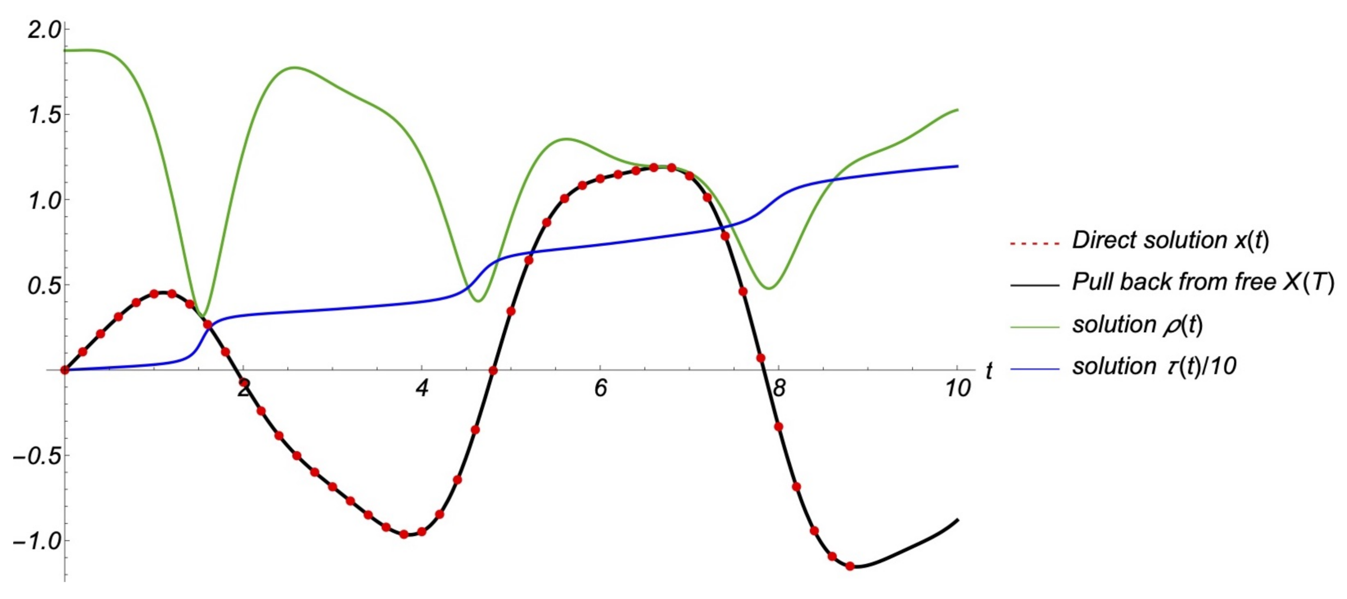
In Section 5.2, we illustrate our theory by the time-dependent Mathieu profile ${\omega }^2\left(t\right)=a-2qcos2t,a,b\mathrm{const}.$, the direct analytic treatment of which is complicated.

2. The Junker–Inomata Derivation of the Propagator

Starting with a general quadratic Lagrangian in 1 + 1 spacetime dimensions with coordinates $\tilde{x}$ and t, Junker and Inomata derived the equation of motion [12]:

$$\ddot{\tilde{x}}+\dot{\lambda }\left(t\right)\dot{\tilde{x}}+{\omega }^2\left(t\right)\tilde{x}=F\left(t\right),$$

(11)

which describes a nonrelativistic particle of unit mass with dissipation $\lambda \left(t\right)$. The driving force $F\left(t\right)$ can be eliminated by subtracting a particular solution $h\left(t\right)$ of (11), $x\left(t\right)=\tilde{x}\left(t\right)-h\left(t\right),$ in terms of which (11) becomes homogeneous,

$$\begin{array}{c}\hfill \ddot{x}+\dot{\lambda }\left(t\right)\dot{x}+{\omega }^2\left(t\right)x=0.\end{array}$$

(12)

This equation can be obtained from the time-dependent generalization of (6),

$$\begin{array}{c}\hfill L_{CK}=\frac{1}{2}{e}^{\lambda \left(t\right)}[{\dot{x}}^2-{\omega }^2\left(t\right)x^2].\end{array}$$

(13)

The friction can be eliminated by setting $x\left(t\right)=y\left(t\right)e^{-\lambda \left(t\right)/2}$, which yields a harmonic oscillator with no friction, but with a shifted frequency [29,30,31],

$$\ddot{y}+{\mathsf{\Omega }}^2\left(t\right)y=0\mathrm{where}{\mathsf{\Omega }}^2\left(t\right)={\omega }^2\left(t\right)-\frac{{\dot{\lambda }}^2\left(t\right)}{4}-\frac{\ddot{\lambda }\left(t\right)}{2}.$$

(14)

For $\lambda \left(t\right)={\lambda }_{0}t$ and $\omega ={\omega }_0=\mathrm{const}.$, for example, we obtain the usual harmonic oscillator with a constant shifted frequency, ${\mathsf{\Omega }}^2={\omega }_0^2-{\lambda }_0^2/4=\mathrm{const}.$

The frequency is in general time-dependent, though $\mathsf{\Omega }=\mathsf{\Omega }\left(t\right)$; therefore, (14) is a Sturm–Liouville equation that can be solved analytically only in exceptional cases.

Junker and Inomata [12] followed another, more subtle path. Equation (12) is a linear equation with time-dependent coefficients, the solution of which can be searched for within the ansatz (A similar transcription was used also by Rezende [28].):

$$x\left(t\right)=\rho \left(t\right)\left(A{e}^{i\overline{\omega }\tau \left(t\right)}+B{e}^{-i\overline{\omega }\tau \left(t\right)}\right),$$

(15)

where A, B, and $\overline{\omega }$ are constants and $\rho \left(t\right)$ and $\tau \left(t\right)$ functions to be found. Inserting (15) into (12), putting the coefficients of the exponentials to zero, separating the real and imaginary parts, and absorbing a new integration constant into $A,B$ provide us with the coupled system for $\rho \left(t\right)$ and $\tau \left(t\right)$,

$$\begin{array}{ccc}& & \ddot{\rho }+\dot{\lambda }\dot{\rho }+({\omega }^2\left(t\right)-{\overline{\omega }}^2{\dot{\tau }}^2)\rho =0,\hfill \end{array}$$

(16)

$$\begin{array}{ccc}& & \dot{\tau }\left(t\right){\rho }^2\left(t\right)e^{\lambda \left(t\right)}=1.\hfill \end{array}$$

(17)

Manifestly, $\dot{\tau }>0$. Inserting $\dot{\tau }$ into (16) then yields the Ermakov–Milne–Pinney (EMP) equation [32,33,34] with time-dependent coefficients,

$$\ddot{\rho }+\dot{\lambda }\dot{\rho }+{\omega }^2\left(t\right)\rho =\frac{e^{-2\lambda \left(t\right)}{\overline{\omega }}^2}{{\rho }^3}.$$

(18)

We note for later use that eliminating $\rho$ would yield instead:

$${\overline{\omega }}^2=\frac{1}{{\dot{\tau }}^2}\left({\omega }^2\left(t\right)-\frac{1}{2}\frac{\stackrel{⃛}{\tau }}{\dot{\tau }}+\frac{3}{4}{\left(\frac{\ddot{\tau }}{\dot{\tau }}\right)}^2-\frac{\ddot{\lambda }}{2}-\frac{{\dot{\lambda }}^2}{4}\right).$$

(19)

Conversely, the constancy of the r.h.s. here can be verified using Equation (17). Equivalently, starting with the Junker–Inomata condition (10),

$${\omega }^2\left(t\right)=\frac{\ddot{f}}{f}-2\frac{{\dot{f}}^2}{f^2}+\frac{{\dot{\lambda }}^2}{4}+\frac{\ddot{\lambda }}{2}.$$

(20)

To sum up, the strategy to follow is [12,35,36]:

• to solve first the EMP Equation (18) for $\rho$;
• to integrate (17),

  $$\tau \left(t\right)={\int }^t\frac{e^{-\lambda \left(u\right)}}{{\rho }^2\left(u\right)}du.$$

  (21)

Then, the trajectory is given by (15).

Junker and Inomata showed, moreover, that substituting into (13) the new coordinates:

$$T=\frac{tan\left[\overline{\omega }\tau \left(t\right)\right]}{\overline{\omega }},X=x{e}^{\frac{\lambda \left(t\right)}{2}}\dot{\tau }{\left(t\right)}^{\frac{1}{2}}sec\left[\overline{\omega }\tau \left(t\right)\right],$$

(22)

allows us to present the Caldirola–Kanai action as (Surface terms do not change the classical equations of motion and multiply the propagator by an unobservable phase factor, and are therefore dropped.),

$${\displaystyle {\mathcal{A}}_{CK}={\int }_{t^{\prime }}^{t^{″}}{L}_{CK}dt={\int }_{T^{\prime }}^{T^{″}}\frac{1}{2}{\left(\frac{dX}{dT}\right)}^{2}dT,}$$

(23)

where we recognize the action of a free particle of unit mass. One checks also directly that $X,T$ satisfy the free equation, as they should. The conditions (10) are readily verified.

The coordinates X and T describe a free particle; therefore, the propagator is (5) (as anticipated by our notation). The clue of Junker and Inomata [12] is that, conversely, trading X and T in (5) for x and t allows deriving the propagator for the CK oscillator (see also [11], Section 5.1) (The extension of (24) from $0<\overline{\omega }({\tau }^{″}-{\tau }^{\prime })<\pi$ to all t [2,3,6,11] is discussed in Section 4.),

$$\begin{array}{ccc}& & K_{osc}(x^{″},t^{″}|x^{\prime },t^{\prime })={\left[\frac{\overline{\omega }{e}^{\frac{{\lambda }^{″}+{\lambda }^{\prime }}{2}}{\left({\dot{\tau }}^{″}{\dot{\tau }}^{\prime }\right)}^{\frac{1}{2}}}{2\pi i\hslash sin\left[\overline{\omega }({\tau }^{″}-{\tau }^{\prime })\right]}\right]}^{\frac{1}{2}}\times \hfill \\ & & exp\left\{\frac{i\overline{\omega }}{2\hslash sin\left[\overline{\omega }({\tau }^{″}-{\tau }^{\prime })\right]}\left[({x″}^2{e}^{{\lambda }^{″}}{\dot{\tau }}^{″}+{x\prime }^2{e}^{{\lambda }^{\prime }}{\dot{\tau }}^{\prime })cos\left[\overline{\omega }({\tau }^{″}-{\tau }^{\prime })\right]-2x^{″}{x}^{\prime }{e}^{\frac{{\lambda }^{″}+{\lambda }^{\prime }}{2}}{\left({\dot{\tau }}^{″}{\dot{\tau }}^{\prime }\right)}^{\frac{1}{2}}\right]\right\},\hfill \end{array}$$

(24)

where we used the shorthands ${\lambda }^{″}=\lambda \left(t^{″}\right),{\tau }^{″}=\tau \left(t^{″}\right)$, etc.

This remarkable formula says that in terms of “redefined time”, $\tau$, the problem is essentially one with a constant frequency. Equation (24) is still implicit, though, as it requires solving first the coupled system (17), which we can do only in particular cases.

• When $\lambda \left(t\right)={\lambda }_{0}t$ where ${\lambda }_0=\mathrm{const}.\ge 0$, Equation (12) describes a time-dependent oscillator with constant friction,

  $$\begin{array}{c}\hfill \ddot{x}+{\lambda }_0\dot{x}+{\omega }^2\left(t\right)x=0.\end{array}$$

  (25)
  Then, setting $R\left(t\right)=\rho \left(t\right)e^{{\lambda }_{0}t/2}$, Equation (17) provide us with the EMP equation for R, cf. (18),

  $$\ddot{R}+{\mathsf{\Omega }}^2\left(t\right)R-\frac{{\overline{\omega }}^2}{R^3}=0,\mathrm{where}{\mathsf{\Omega }}^2\left(t\right)={\omega }^2\left(t\right)-\frac{{\lambda }_0^2}{4};$$

  (26)
• If, in addition, the frequency is constant $\omega \left(t\right)={\omega }_0=\mathrm{const}.,$ then Equation (26) is solved algebraically by:

  $${\overline{\omega }}^2={\omega }_0^2-{\lambda }_0^2/4,R=1\Rightarrow \rho \left(t\right)=e^{-{\lambda }_{0}t/2},\tau \left(t\right)=t.$$

  (27)
  Thus, $x\left(t\right)$ is a linear combination of $e^{-\frac{1}{2}{\lambda }_{0}t}sin\overline{\omega }t$ and $e^{-\frac{1}{2}{\lambda }_{0}t}cos\overline{\omega }t.$ The spacetime coordinate transformation of $(x,t)\to (X,T)$ in (22) simplifies to the friction-generalized form of that of Niederer [16],

  $$\begin{array}{c}\hfill T=\frac{tan\left(\overline{\omega }t\right)}{\overline{\omega }},X=xexp\left(\frac{1}{2}{\lambda }_{0}t\right)sec\left(\overline{\omega }t\right),\end{array}$$

  (28)

  for which the general expression (24) reduces to (9) when ${\lambda }_0=0$;
• When the oscillator is turned off, ${\omega }_0=0$, but ${\lambda }_0>0$, we have motion in a dissipative medium. The coordinate transformation propagator (22) and (24) become:

  $$X=\frac{2x}{1+exp\left(-{\lambda }_{0}t\right)},T=\frac{2}{{\lambda }_0}\frac{1-exp(-{\lambda }_{0}t)}{1+exp(-{\lambda }_{0}t)}$$

  (29)

  and:

  $$\begin{array}{ccc}{K}_{diss}(x^{″},t^{″}|x^{\prime },t^{\prime })\hfill & =\hfill & {\left[{\displaystyle \frac{{\lambda }_0}{2\pi i\hslash [exp(-{\lambda }_0{t}^{\prime })-exp(-{\lambda }_0{t}^{″})]}}\right]}^{\frac{1}{2}}\hfill \\ & \hfill & \times exp\left\{{\displaystyle \frac{i{\lambda }_0}{2\hslash }\frac{{(x^{″}-x^{\prime })}^2}{exp(-{\lambda }_0{t}^{\prime })-exp(-{\lambda }_0{t}^{″})}}\right\},\hfill \end{array}$$

  (30)

  respectively. A driving force $F_0$ (e.g., terrestrial gravitation) could be added and then removed by $x\to x+(F_0/{\lambda }_0)t$.

Further examples can be found in [13,14,15]. An explicitly time-dependent example is presented in Section 5.2.

3. The Eisenhart–Duval Lift

Further insight can be gained by “Eisenhart–Duval (E-D) lifting” the system to one higher dimension to what is called a “Bargmann space” [17,18,19,20,21]. The latter is a $d+1+1$-dimensional manifold endowed with a Lorentz metric, the general form of which is:

$$g_{\mu \nu }d{x}^{\mu }d{x}^{\nu }=g_{ij}(x,t)d{x}^{i}d{x}^j+2dtds-2V(x,t)d{t}^2,$$

(31)

which carries a covariantly constant null Killing vector ${\partial }_s$. Then:

Theorem 1

([18,20]). Factoring out the foliation generated by ${\partial }_s$ yields a nonrelativistic spacetime in $d+1$ dimensions. Moreover, the null geodesics of the Bargmann metric $g_{\mu \nu }$ project to ordinary spacetime, consistent with Newton’s equations. Conversely, if $\left(\gamma \right(t),t)$ is a solution of the nonrelativistic equations of motion, then its null lifts to Bargmann space are:

$$\left(\gamma \left(t\right),t,s\left(t\right)\right),s\left(t\right)=s_0-\mathcal{A}\left(\gamma \right)=s_0-{\int }^{t}L(\gamma \left(r\right),r)dr$$

(32)

where $s_0$ is an arbitrary initial value.

Let us consider, for example, a particle of unit mass with the Lagrangian of:

$${\displaystyle L=\frac{1}{2\alpha \left(t\right)}{g}_{ij}\left(x^k\right){\dot{x}}^i{\dot{x}}^j-\beta \left(t\right)V(x^i,t),}$$

(33)

where $g_{ij}\left(x^k\right)d{x}^{i}d{x}^j$ is a positive metric on a curved configuration space Q with local coordinates $x^i$, $i=1,\dots ,d$. The coefficients $\alpha \left(t\right)$ and $\beta \left(t\right)$ may depend on time t, and $V(x^i,t)$ is some (possibly time-dependent) scalar potential. The associated equations of motion are:

$$\frac{d^2{x}^i}{d{t}^2}+{\mathsf{\Gamma }}_{jk}^i\frac{d{x}^j}{dt}\frac{d{x}^k}{dt}-\frac{\dot{\alpha }}{\alpha }\frac{d{x}^i}{dt}=-\alpha \beta g^{ij}{\partial }_{j}V,$$

(34)

where the ${\mathsf{\Gamma }}_{jk}^i$ are the Christoffel symbols of the metric $g_{ij}$. For $d=1$, $g_{ij}={\delta }_{ij}$ and $V=\frac{1}{2}{\omega }^2\left(t\right)x^2$ for $\alpha =\beta =1$, resp. for $\alpha ={\beta }^{-1}=e^{-\lambda \left(t\right)}$, we obtain a (possible time-dependent) 1d oscillator without, resp. with, friction, Equation (7) [7,8,9,29,30,31].

Equation (34) can also be obtained by projecting a null-geodesic of $d+1+1$-dimensional Bargmann spacetime with coordinates $\left(x^{\mu }\right)=(x^i,t,s)$, whose metric is:

$$g_{\mu \nu }d{x}^{\mu }d{x}^{\nu }=\frac{1}{\alpha }{g}_{ij}d{x}^{i}d{x}^j+2dtds-2\beta Vd{t}^2.$$

(35)

For $\alpha ={\beta }^{-1}=e^{-\lambda \left(t\right)}$, we recover (12).

Choosing $\lambda \left(t\right)=lnm\left(t\right)$ would describe motion with a time-dependent mass $m\left(t\right)$. The friction can be removed by the conformal rescaling $x\to y=\sqrt{m}x$, and the null geodesics of the rescaled metric describe, consistent with (14), an oscillator with no friction, but with a time-dependent frequency, ${\mathsf{\Omega }}^2={\omega }^2-\frac{\ddot{m}}{2m}+(\frac{\dot{m}}{2m}{)}^2$ [37].

The friction term $-(\dot{\alpha }/\alpha ){\dot{x}}^i$ in (34) can be removed also by introducing a new time parameter $\tilde{t}$, defined by $d\tilde{t}=\alpha dt$ [21]. For $\lambda \left(t\right)={\lambda }_{0}t$, for example, putting $\tilde{t}=-e^{-{\lambda }_{0}t}/{\lambda }_0$ eliminates the friction, but it does this at the price of obtaining a manifestly time-dependent frequency [38,39]:

$$\frac{d^{2}x}{d{\tilde{t}}^2}+{\tilde{\mathsf{\Omega }}}^2\left(\tilde{t}\right)x=0,{\tilde{\mathsf{\Omega }}}^2\left(\tilde{t}\right)=\frac{{\omega }^2}{{\tilde{t}}^2{\lambda }_0^2}.$$

(36)

3.1. The Junker–Inomata Ansatz as a Conformal Transformation

The approach outlined in Section 2 admits a Bargmannian interpretation. For simplicity, we only consider the frictionless case $\lambda =0$.

Theorem 2.

The Junker–Inomata method of converting the time-dependent system into one with a constant frequency by switching from “real” to “fake time”,

$$t\to \tau \left(t\right),\xi =\dot{\tau }x$$

(37)

induces a conformal transformation between the Bargmann metrics:

$$\begin{array}{cccc}\hfill & d{x}^2+2dtds-{\omega }^2\left(t\right)x^{2}d{t}^2\hfill & \hfill \mathit{frequency}& {\omega }^2\left(t\right)\hfill \end{array}$$

(38a)

$$\begin{array}{cccc}\hfill & d{\xi }^2+2d\tau d\sigma -{\overline{\omega }}^2{\xi }^{2}d{\tau }^2,\hfill & \hfill \mathit{frequency}& \overline{\omega }=\mathrm{const}.\hfill \end{array}$$

(38b)

$$d{\xi }^2+2d\tau d\sigma -{\overline{\omega }}^2{\xi }^{2}d{\tau }^2=\dot{\tau }\left(t\right)\left(d{x}^2+2dtds-{\omega }^2\left(t\right)x^{2}d{t}^2\right).$$

(39)

Proof. 

Putting $\mu =ln\dot{\tau }$ allows us to present the constant-frequency $\overline{\omega }$ (19) as:

$${\overline{\omega }}^2={\dot{\tau }}^{-2}\left({\omega }^2\left(t\right)-\frac{1}{2}\ddot{\mu }+\frac{1}{4}{\dot{\mu }}^2\right).$$

(40)

Then, with the notation $\stackrel{\circ }{\zeta }$= dζ/dτ, we find,

$${\stackrel{\circ }{\zeta }}^2={\dot{\tau }}^{-1}\left[{\dot{x}}^2+\frac{1}{4}{\dot{\mu }}^2{x}^2-\frac{1}{2}\ddot{\mu }{x}^2+\frac{d}{dt}\left(\frac{1}{2}\dot{\mu }{x}^2\right)\right].$$

Let us now recall that the null lift to the Bargmann space of a spacetime curve is obtained by subtracting the classical action as the vertical coordinate,

$$\begin{array}{c}\hfill d\sigma =-L(\xi ,\stackrel{\circ }{\xi },\tau )d\tau =-\frac{1}{2}({\stackrel{\circ }{\xi }}^2-{\overline{\omega }}^2{\xi }^2)d\tau \end{array}$$

(41)

Setting here $\xi =x\phantom{(}{\dot{\tau }}^{1/2}$ and dropping surface terms yield, using the same procedure for the time-dependent-frequency case,

$$d\sigma =ds=-\frac{1}{2}\left({\dot{x}}^2-{\omega }^2\left(t\right)x^2\right)dt$$

(42)

up to surface terms. Then, inserting all our formulae into (38a) and (38b) yields (39), as stated. In Junker–Inomata language (10), $f\left(t\right)={\dot{\tau }}^{1/2}sec\left(\overline{\omega }\tau \right),g\left(t\right)={\left(\overline{\omega }\right)}^{-1}tan\left(\overline{\omega }\tau \right)$. □

Our investigation has so far concerned classical aspects. Now, we consider what happens quantum mechanically. Restricting our attention at $d=1$ space dimensions as before (In $d>2$, conformal invariance requires adding a scalar curvature term to the Laplacian.), we posit that the E-D lift $\tilde{\psi }$ of a wave function $\psi$ is equivariant,

$$\tilde{\psi }(x,t,s)=e^{\frac{i}{\hslash }s}\psi (x,t)\Rightarrow {\partial }_s\tilde{\psi }=\frac{i}{\hslash }\tilde{\psi }.$$

(43)

Then, the massless Klein–Gordon equation for $\tilde{\psi }$ associated with the $1+1+1=3$ d Barmann metric implies the Schrödinger equation in 1+1 d,

$${\Delta }_g\tilde{\psi }=0\Rightarrow i{\partial }_t\psi =\left[-\frac{{\hslash }^2}{2}{\Delta }_x+V(x,t)\right]\psi$$

(44)

where ${\Delta }_g$ is the Laplace–Beltrami operator associated with the metric. In $d=1$, it is of course ${\Delta }_x={\partial }_x^2$.

A conformal diffeomorphism $(X,T,S)\to \tilde{f}(X,T,S)=(x,t,s)$ with conformal factor ${\sigma }_f^2$, ${\tilde{f}}^{*}{g}_{\mu \nu }={\sigma }_f^2{g}_{\mu \nu },$ projects to a spacetime transformation $(X,T)\to f(X,T)=(x,t)$. It is implemented on a wave function lifted to the Bargmann space as:

$$\tilde{\psi }(x,t,s)={\sigma }_f^{-1/2}\tilde{\psi }(X,T,S)$$

(45)

In Section 4.2, these formulae are applied to the Niederer map (73).

3.2. The Arnold Map

The general damped harmonic oscillator with time-dependent driving force $F\left(t\right)$ in 1 + 1 dimensions, (11),

$$\ddot{x}+\dot{\lambda }\dot{x}+{\omega }^2\left(t\right)x=F\left(t\right),$$

(46)

can be solved by an Arnold transformation [22,23], which “straightens the trajectories” [21,29,30,31,40]. To this end, one introduces new coordinates,

$$T=\frac{u_1}{u_2},X=\frac{x-u_p}{u_2},$$

(47)

where $u_1$ and $u_2$ are solutions of the associated homogeneous Equation (46) with $F\equiv 0$ and $u_p$ is a particular solution of the full Equation (46). It is worth noting that (47) allows checking, independently, the Junker–Inomata criterion in (10). The initial conditions are chosen as,

$$u_1\left(t_0\right)={\dot{u}}_2\left(t_0\right)=0,{\dot{u}}_1\left(t_0\right)=u_2\left(t_0\right)=1,u_p\left(t_0\right)={\dot{u}}_p\left(t_0\right)=0.$$

(48)

Then, in the new coordinates, the motion becomes free [22,23],

$$X\left(T\right)=aT+b,a,b=\mathrm{const}.$$

(49)

Equation (46) can be obtained by projecting a null geodesic of the Bargmann metric:

$$g_{\mu \nu }d{x}^{\mu }d{x}^{\nu }=e^{\lambda \left(t\right)}d{x}^2+2dtds-2e^{\lambda \left(t\right)}\left(\frac{1}{2}\omega {\left(t\right)}^2{x}^2-F\left(t\right)x\right)d{t}^2.$$

(50)

Completing (47) by:

$$S=s+e^{\lambda }{u}_2^{-1}\left(\frac{1}{2}{\dot{u}}_2{x}^2+{\dot{u}}_{p}x\right)+g\left(t\right)\mathrm{where}\dot{g}=\frac{1}{2}{e}^{\lambda }\left({\dot{u}}_p^2-{\omega }^2{u}_p^2+2F{u}_p\right)$$

(51)

lifts the Arnold map to Bargmann spaces, $(x,t,s)\to (X,T,S)$ (In the Junker–Inomata setting (10), $f=u_2{e}^{-\lambda /2}$ and $g\left(t\right)=u_1/u_2$.),

$$g_{\mu \nu }d{x}^{\mu }d{x}^{\nu }=e^{\lambda \left(t\right)}{u}_2^2\left(t\right)\left(d{X}^2+2dTdS\right).$$

(52)

The oscillator metric (50) is thus carried conformally to the free one, generalizing earlier results [18,19,41]. For the damped harmonic oscillator with $\lambda \left(t\right)={\lambda }_{0}t$ and $F\left(t\right)\equiv 0$, $u_p\equiv 0$ is a particular solution. When $\omega ={\omega }_0=\mathrm{const}.$, for example,

$$u_1=e^{-{\lambda }_{0}t/2}\frac{sin{\mathsf{\Omega }}_{0}t}{{\mathsf{\Omega }}_0},u_2=e^{-{\lambda }_{0}t/2}\left(cos{\mathsf{\Omega }}_{0}t+\frac{{\lambda }_0}{2{\mathsf{\Omega }}_0}sin{\mathsf{\Omega }}_{0}t\right),{\mathsf{\Omega }}_0^2={\omega }_0^2-{\lambda }_0^2/4$$

(53)

are two independent solutions of the homogeneous equation with initial conditions (48) and provide us with:

$$\begin{array}{ccc}\hfill T& & =\frac{sin{\mathsf{\Omega }}_{0}t}{{\mathsf{\Omega }}_0(cos{\mathsf{\Omega }}_{0}t+\frac{{\lambda }_0}{2{\mathsf{\Omega }}_0}sin{\mathsf{\Omega }}_{0}t)},\hfill \end{array}$$

(54)

$$\begin{array}{ccc}\hfill X& & =\frac{e^{{\lambda }_{0}t/2}x}{cos{\mathsf{\Omega }}_{0}t+\frac{{\lambda }_0}{2{\mathsf{\Omega }}_0}sin{\mathsf{\Omega }}_{0}t},\hfill \end{array}$$

(55)

$$\begin{array}{ccc}\hfill S& & =s-\frac{1}{2}{e}^{{\lambda }_{0}t}{x}^2\left(\frac{{\omega }_0^2}{{\mathsf{\Omega }}_0}\right)\frac{sin{\mathsf{\Omega }}_{0}t}{cos{\mathsf{\Omega }}_{0}t+\frac{{\lambda }_0}{2{\mathsf{\Omega }}_0}sin{\mathsf{\Omega }}_{0}t}.\hfill \end{array}$$

(56)

In the undamped case, ${\lambda }_0=0$; thus, ${\mathsf{\Omega }}_0={\omega }_0$, and (56) reduces to that of Niederer [16] lifted to the Bargmann space [19,20],

$$T=\frac{tan{\omega }_{0}t}{{\omega }_0},X=\frac{x}{cos{\omega }_{0}t},S=s-\frac{1}{2}{x}^2{\omega }_{0}tan{\omega }_{0}t.$$

(57)

The Junker–Inomata construction in Section 2 can be viewed as a particular case of the Arnold transformation. We chose $u_p\equiv 0$ and the two independent solutions:

$$u_1=e^{-\lambda /2}{\dot{\tau }}^{-1/2}\frac{sin\overline{\omega }\tau }{\overline{\omega }},u_2=e^{-\lambda /2}{\dot{\tau }}^{-1/2}cos\overline{\omega }\tau .$$

(58)

The initial conditions (48) at $t_0=0$ imply $\tau \left(0\right)=\dot{\rho }\left(0\right)=0,\rho \left(0\right)=\dot{\tau }\left(0\right)=1.$ Then, spelling out (51),

$$S=s-\frac{1}{2}{e}^{\lambda }\left(\overline{\omega }\dot{\tau }tan\overline{\omega }\tau +\frac{1}{2}\dot{\lambda }+\frac{1}{2}\frac{\ddot{\tau }}{\dot{\tau }}\right)x^2$$

(59)

completes the lift of (22) to Bargmann spaces. In conclusion, the one-dimensional damped harmonic oscillator is described by the conformally flat Bargmann metric,

$$g_{\mu \nu }d{x}^{\mu }d{x}^{\nu }=\frac{{cos}^2\overline{\omega }\tau }{\dot{\tau }}\left(d{X}^2+2dTdS\right).$$

(60)

The metric (60) is manifestly conformally flat; therefore, its geodesics are those of the free metric, $X\left(T\right)=aT+b$. Then, using (47) with (58) yields:

$$x\left(t\right)=e^{-\lambda \left(t\right)/2}{\dot{\tau }}^{-1/2}\left(t\right)\left(a\frac{sin\left[\overline{\omega }\tau \left(t\right)\right]}{\overline{\omega }}+bcos\left[\overline{\omega }\tau \left(t\right)\right]\right).$$

(61)

The bracketed quantity here describes a constant-frequency oscillator with “time” $\tau \left(t\right)$. The original position, x, obtains a time-dependent “conformal” scale factor.

4. The Maslov Correction

As mentioned before, the semiclassical formula (9) is correct only in the first oscillator half-period, $0<t^{″}-t^{\prime }<\pi /{\mathsf{\Omega }}_0$. Its extension for all t involves the Maslov correction. In the constant-frequency case with no friction, for example, assuming that ${\mathsf{\Omega }}_0(t^{″}-t^{″})/\pi$ is not an integer, we have [2,3,6],

$$\begin{array}{ccc}\hfill K^{ext}(x^{″},t^{″}|x^{\prime },t^{\prime })& =& {\left[\frac{{\mathsf{\Omega }}_0}{2\pi \hslash |sin{\mathsf{\Omega }}_0(t^{″}-t^{\prime })|}\right]}^{\frac{1}{2}}\times e^{-i\frac{\pi }{4}(1+2\ell )}\hfill \\ & & exp\left\{\frac{i{\mathsf{\Omega }}_0}{2\hslash sin{\mathsf{\Omega }}_0(t^{″}-t^{\prime })}\left[({x^{″}}^2+{x^{\prime }}^2)cos{\mathsf{\Omega }}_0(t^{″}-t^{\prime })-2x^{″}{x}^{\prime }\right]\right\},\hfill \end{array}$$

(62)

where the integer:

$$\ell =\mathrm{Ent}\left[\frac{{\mathsf{\Omega }}_0(t^{″}-t^{\prime })}{\pi }\right]$$

(63)

is called the Maslov index ($\mathrm{Ent}\left[x\right]$ is the integer part of x.). ℓ counts the completed half-periods and is related also to the Morse index, which counts the negative modes of ${\partial }^2\mathcal{A}/\partial x^{\prime }\partial x^{″}$ [4,5].

Now, we generalize (62) to the time-dependent frequency:

Theorem 3.In terms of $\overline{\omega }$ and τ introduced in Section 2,

• Outside caustics, i.e., for $\overline{\omega }({\tau }^{″}-{\tau }^{\prime })\ne \pi \ell$, the propagator for the harmonic oscillator with the time-dependent frequency and friction is: -4.6cm0cm

  $$\begin{array}{ccc}& & K^{ext}(x^{″},t^{″}|x^{\prime },t^{\prime })={\left[\frac{\overline{\omega }{e}^{\frac{{\lambda }^{″}+{\lambda }^{\prime }}{2}}{\left({\dot{\tau }}^{″}{\dot{\tau }}^{\prime }\right)}^{\frac{1}{2}}}{2\pi \hslash |sin\overline{\omega }({\tau }^{″}-{\tau }^{\prime })|}\right]}^{1/2}exp\left\{-\frac{i\pi }{2}\left(\frac{1}{2}+\mathrm{Ent}\left[\frac{\overline{\omega }({\tau }^{″}-{\tau }^{\prime })}{\pi }\right]\right)\right\}\hfill \\ & & \times exp\left\{\frac{i\overline{\omega }}{2\hslash sin\overline{\omega }({\tau }^{″}-{\tau }^{\prime })}[(x^{″2}{e}^{{\lambda }^{″}}{\dot{\tau }}^{″}+x^{\prime 2}{e}^{{\lambda }^{\prime }}{\dot{\tau }}^{\prime })cos\left[\overline{\omega }({\tau }^{″}-{\tau }^{\prime })\right]-2x^{″}{x}^{\prime }{e}^{\frac{{\lambda }^{″}+{\lambda }^{\prime }}{2}}{\left({\dot{\tau }}^{″}{\dot{\tau }}^{\prime }\right)}^{\frac{1}{2}}]\right\};\hfill \end{array}$$

  (64)
• At caustics, i.e., for:

  $$\overline{\omega }({\tau }^{″}-{\tau }^{\prime })=\pi \ell ,\ell =0,\pm 1,\cdots$$

  (65)
  we have instead [3,6],

  $$\begin{array}{ccc}& & K^{ext}\left(x^{″},x^{\prime },|{\tau }^{″}-{\tau }^{\prime }=\frac{\pi }{\overline{\omega }}\ell \right)={\left[e^{\frac{{\lambda }^{″}+{\lambda }^{\prime }}{2}}{\left({\dot{\tau }}^{″}{\dot{\tau }}^{\prime }\right)}^{\frac{1}{2}}\right]}^{1/2}\hfill \\ & & \times exp\left(-\frac{i\pi \ell }{2}\right)\delta \left(x^{\prime }exp({\lambda }^{\prime }/2){\dot{\tau }}^{\prime 1/2}-{(-1)}^k{x}^{″}exp({\lambda }^{″}/2){\dot{\tau }}^{″1/2}\right).\hfill \end{array}$$

  (66)

Proof. 

In terms of the redefined coordinates:

$$\tau =\tau \left(t\right)\mathrm{and}\xi =xexp\left[\frac{\lambda \left(t\right)}{2}\right]{\dot{\tau }}^{1/2}\left(t\right),$$

(67)

cf. (37), and using the notation $\stackrel{\circ }{\{·\}}$ = d/dτ, the time-dependent oscillator Equation (12) is taken into:

$$\stackrel{\circ \circ }{\xi }+{\overline{\omega }}^2\xi =0,\hspace{1em}\mathrm{where}\hspace{1em}{\overline{\omega }}^2=\frac{1}{{\dot{\tau }}^2}({\omega }^2(t)-\frac{1}{2}\frac{\stackrel{⃛}{\tau }}{\dot{\tau }}+\frac{3}{4}{\left(\frac{\ddot{\tau }}{\dot{\tau }}\right)}^2-\frac{\ddot{\lambda }}{2}-\frac{{\dot{\lambda }}^2}{4}).$$

(68)

Thus, the problem is reduced to one with a time-independent frequency, $\overline{\omega }$ in (19) (We record for the sake of later investigations that (turning off $\lambda$) (Section 4) can be presented as:

$${\omega }^2\left(t\right)-{\dot{\tau }}^2{\overline{\omega }}^2=\frac{1}{2}\mathit{S}\left(\tau \right)$$

(69)

where $\mathit{S}\left(\tau \right)=\frac{\stackrel{⃛}{\tau }}{\dot{\tau }}-\frac{3}{2}{\left(\frac{\ddot{\tau }}{\dot{\tau }}\right)}^2$ is the Schwarzian derivative of $\tau$ [42]). □

Let us now recall Formula (19) of Junker and Inomata in [12], which tells us how propagators behave under the coordinate transformation $(\xi ,\tau )⟷(x,t)$:

$$\begin{array}{c}\hfill K_2(x^{″},t^{″}|x^{\prime },t^{\prime })={\left[\left(\frac{\partial {\xi }^{\prime }}{\partial x^{\prime }}\right)\left(\frac{\partial {\xi }^{″}}{\partial x^{″}}\right)\right]}^{\frac{1}{2}}{K}_1({\xi }^{″},{\tau }^{″}|{\xi }^{\prime },{\tau }^{\prime }).\end{array}$$

(70)

Here, $K_2=K^{ext}$ is the propagator of an oscillator with a time-dependent frequency and friction, $\omega \left(t\right)$ and $\lambda \left(t\right)$, respectively—the one we are trying to find. $K_1$ is in turn the Maslov-extended propagator of an oscillator with no friction and a constant frequency, as in (62). Then, the propagator for the harmonic oscillator with a time-dependent frequency and friction, Equation (64), is obtained using (67).

Notice that (64) is regular at the points $r_k\in J_k$ where $sin=\pm 1$. However, at caustics, ${\tau }^{″}-{\tau }^{\prime }=(\pi /\overline{\omega })\ell$, $K^{ext}$ diverges, and we have instead (66).

Henceforth, we limit our investigations to $\lambda =0$.

4.1. Properties of the Niederer Map

More insight is gained from the perspective of the generalized Niederer map (22). We first study their properties in some detail. For simplicity, we chose, in the rest of this section, $x^{\prime }=t^{\prime }=0$ and $x^{″}\equiv x$ and $t^{″}\equiv t$.

We start with the observation that the Niederer map (22) becomes singular where the cosine vanishes, i.e., where:

$$cos\left[\overline{\omega }\tau \left(r_k\right)\right]=0,\mathrm{i}.\mathrm{e}.\tau \left(r_k\right)=(k+\frac{1}{2})\frac{\pi }{\overline{\omega }},k=0,\pm 1,\cdots$$

(71)

$r_k<r_{k+1}$ because $\tau \left(t\right)$ is an increasing function by (21). Moreover, each interval:

$$I_k=\left[r_k,r_{k+1}\right],k=0,\pm 1,\cdots$$

(72)

is mapped by (22) onto the full range $-\infty <T<\infty$. Therefore, the inverse mapping is multivalued, labeled by integers k,

$$N_k:T\to t=\frac{{arctan}_k\overline{\omega }T}{\overline{\omega }},X\to x=\frac{X}{\sqrt{1+{\overline{\omega }}^2{T}^2}},$$

(73)

where ${arctan}_k(·)={arctan}_0(·)+k\pi$ with ${arctan}_0(·)$ the principal determination, i.e., in $(-\pi /2,\pi /2)$.

Then, ${lim}_{t\to r_k-}tant=\infty$ and ${lim}_{t\to r_k+}tant=-\infty$ imply that:

$$\underset{T\to \infty }{lim}{N}_k\left(T\right)=r_{k+1}=\underset{T\to -\infty }{lim}{N}_{k+1}\left(T\right).$$

(74)

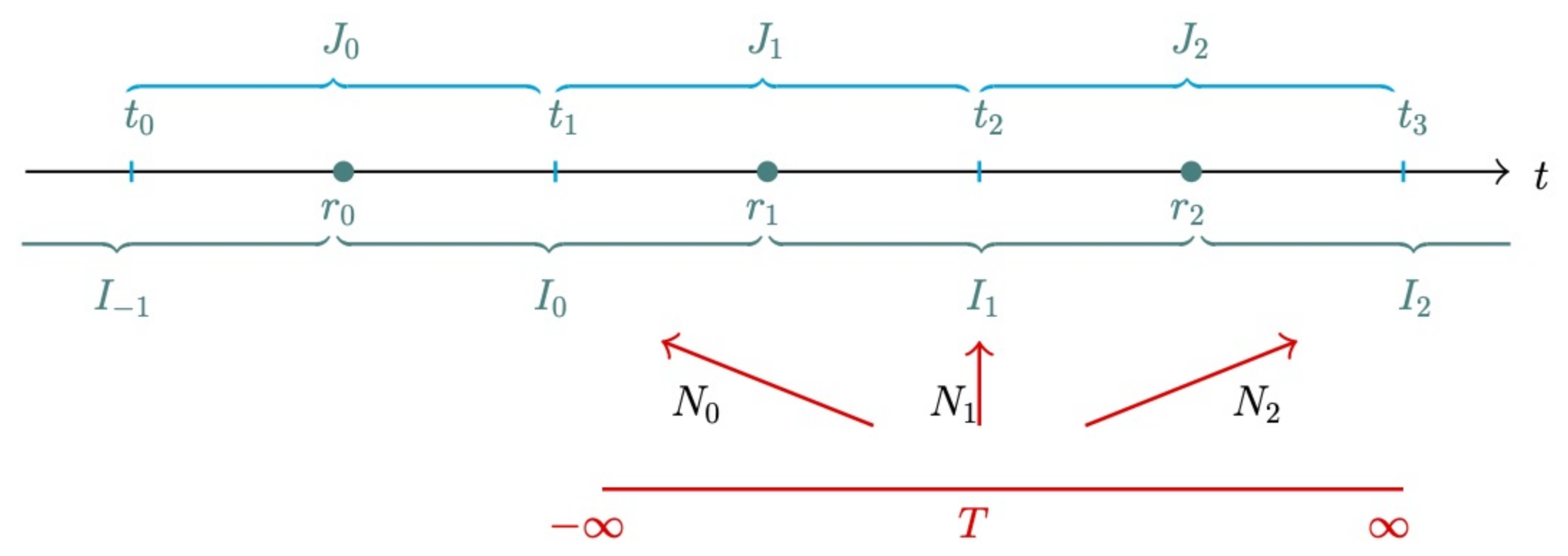
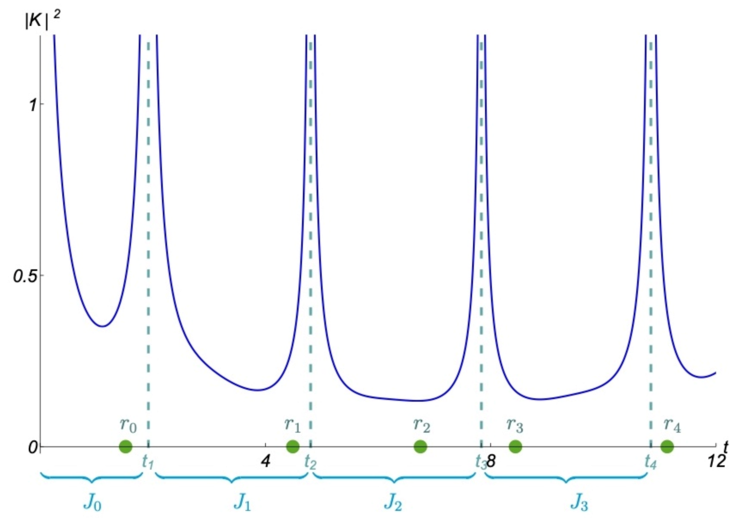
Therefore, the intervals $I_k$ and $I_{k+1}$ are joined at $r_{k+1},$ and the $I_k$ form a partition of the time axis, $\left\{-\infty <t<\infty \right\}={\cup }_k{I}_k.$

Returning to (64) (which is (62) with ${\mathsf{\Omega }}_0\Rightarrow \overline{\omega },t\Rightarrow \tau$), we then observe that, whereas the propagator is regular at $r_k$, it diverges at caustics,

$$sin\left[\overline{\omega }\tau \left(t_{\ell }\right)\right]=0\mathrm{i}.\mathrm{e}.,\tau \left(t_{\ell }\right)=\frac{\pi }{\overline{\omega }}\ell ,\ell =0,\pm 1,\cdots ,$$

(75)

cf. (65). Thus, $t_{\ell }\le t_{\ell +1}$, and:

$$N_k(-\infty )=r_k,N_k(T=0)=t_{k+1},N_k(+\infty )=r_{k+1}.$$

(76)

Thus, $N_k$ maps the full T-line into $I_k$ with $t_k$ an internal point. Conversely, $r_k$ is an internal point of $J_k$. The intervals $J_{\ell }=\left[t_{\ell },t_{\ell +1}\right]$ cover again the time axis, ${\displaystyle {\cup }_{\ell }{J}_{\ell }=\left\{-\infty <t<\infty \right\}.}$

By (61) the classical trajectories are regular at $t=r_k$. Moreover, for arbitrary initial velocities,

$$\sqrt{\dot{\tau }\left(t_{\ell +1}\right)}x\left(t_{\ell +1}\right)=-\sqrt{\dot{\tau }\left(t_{\ell }\right)}x\left(t_{\ell }\right)$$

(77)

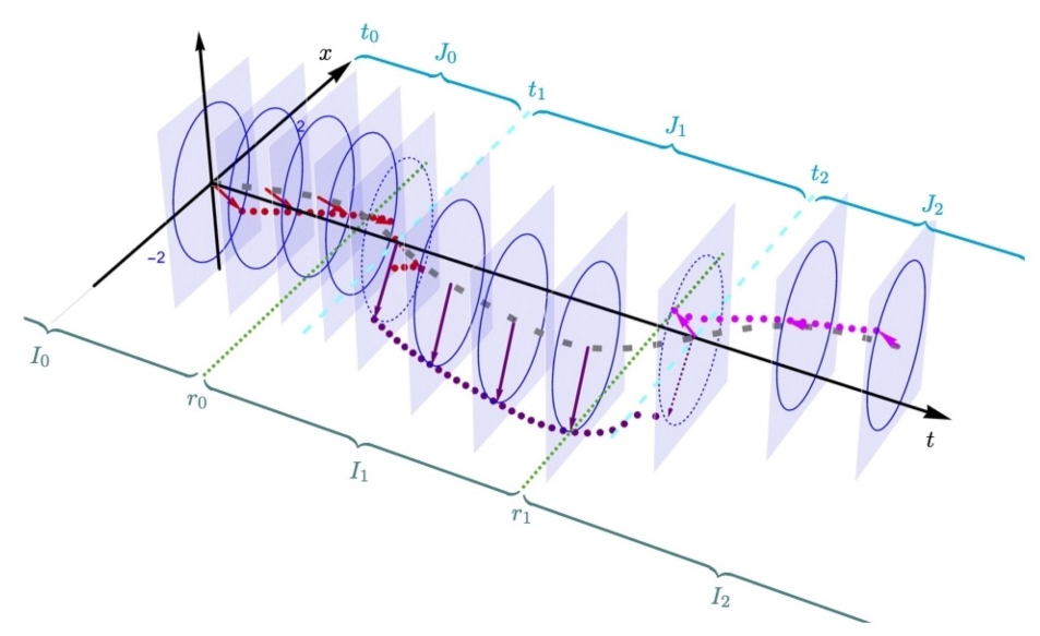
implying that after a half-period $\overline{\omega }\tau \to \overline{\omega }\tau +\pi$, all classical motions are focused at the same point. The two entangled sets of intervals are shown in Figure 1.

The Niederer map (57) “E-D lifts” to the Bargmann space.

Theorem 4.

The E-D lift of the inverse of the Niederer map (57), which we shall denote by ${\tilde{N}}_k:(X,T,S)\to (x,t,s)$ ($t\in I_k$), is:

$$t=\frac{{arctan}_k\overline{\omega }T}{\overline{\omega }},x=\frac{X}{\sqrt{1+{\overline{\omega }}^2{T}^2}},s=S+\frac{X^2}{2}\frac{{\overline{\omega }}^{2}T}{1+{\overline{\omega }}^2{T}^2}.$$

(78)

Proof. 

These formulae follow at once by inverting (57), at once with the cast ${\omega }_0\Rightarrow \overline{\omega },t\Rightarrow \tau$. Alternatively, it could also be proven as for Theorem 2.

For each integer k (78) maps the real line $-\infty <T<\infty$ into the “open strip” [19] $\left[r_k,r_{k+1}\right]\times {\mathbb{R}}^2\equiv I_k\times {\mathbb{R}}^2$ with $r_k$ defined in (71). Their union covers the entire Bargmann manifold of the oscillator. □

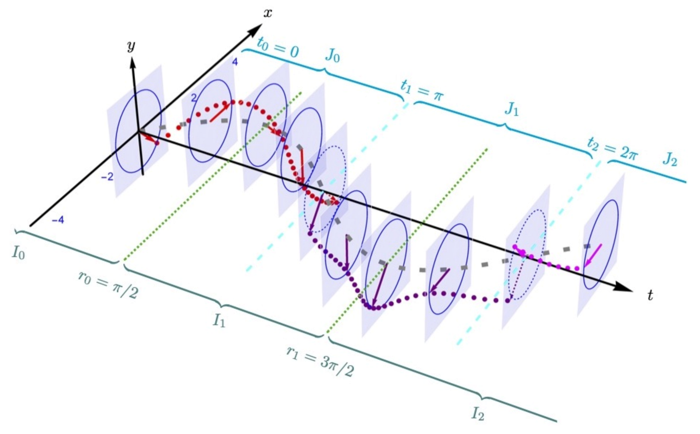
Now, we pull back the free dynamics by the multivalued inverse (78). We put $\overline{\omega }=1$ for simplicity. The free motion with initial condition $X\left(0\right)=0$,

$$X\left(T\right)=aT,S\left(T\right)=S_0-\frac{a^2}{2}T,$$

(79)

E-D lifts by (78) to:

$$x\left(t\right)=asints\left(t\right)=S_0-\frac{a^2}{4}sin2t,$$

(80)

consistent with $s\left(t\right)=s_0-{\overline{\mathcal{A}}}_{osc}$, as can be checked directly. Note that the s coordinate oscillates with a doubled frequency.

• At $t=r_k=(\frac{1}{2}+k)\pi$ (where the Niederer maps are joined), we have ${lim}_{t\to r_k}x\left(t\right)={(-1)}^{k+1}a,{lim}_{t\to r_k}s\left(t\right)=S_0.$ Thus, the pull backs of the Bargmann lifts of free motions are glued to smooth curves;
• Similarly, at t caustics $t=t_{\ell }=\pi \ell$, we infer from (80) that for all initial velocities a and for all ℓ ${lim}_{t\to t_{\ell }}x\left(t\right)=0,{lim}_{t\to t_{\ell }}s\left(t\right)=S_0.$ Thus, the lifts are again smooth at $t_{\ell }$, and after each half-period, all motions are focused above the initial position $(x\left(0\right)=0,s\left(0\right)=S_0)$.

4.2. The Propagator by the Niederer Map

Now, we turn to quantum dynamics. Our starting point is the free propagator (5), which (as mentioned before) is valid only for $0<T^{″}-T^{\prime }$. Its extension to all T involves the sign of $(T^{″}-T^{\prime })$ [19].

Let us explain this subtle point in some detail. First of all, we notice that the usual expression (5) involves a square root, which is double-valued, obliging us to choose one of its branches. Which one we choose is irrelevant: it is a mere gauge choice. However, once we do choose one, we must stick to our choice. Take, for example, the one for which $\sqrt{-i}=e^{-i\pi /4}$, then the prefactor in (5) is:

$${\left[\frac{1}{2\pi i\hslash (T^{″}-T^{\prime })}\right]}^{1/2}=e^{-i\pi /4}{\left[\frac{1}{2\pi \hslash |T^{″}-T^{\prime }|}\right]}^{1/2}.$$

Let us now consider what happens when $T^{″}-T^{\prime }$ changes sign. Then, the prefactor becomes multiplied by $\sqrt{-1}$ so it becomes, for the same choice of the square root,

$$e^{i\pi /2}{e}^{-i\pi /4}{\left[\frac{1}{2\pi \hslash |T^{″}-T^{\prime }|}\right]}^{1/2}=e^{+i\pi /4}{\left[\frac{1}{2\pi \hslash |T^{″}-T^{\prime }|}\right]}^{1/2}.$$

(81)

In conclusion, the formula valid for all T is,

$$\begin{array}{c}\hfill K_{free}(X^{″},T^{″}|X^{\prime },T^{\prime })=e^{-i\frac{\pi }{4}\mathrm{sign}(T^{″}-T^{\prime })}{\left[{\displaystyle \frac{1}{2\pi \hslash |T^{″}-T^{\prime }|}}\right]}^{1/2}exp\left\{{\displaystyle \frac{i}{\hslash }{\overline{\mathcal{A}}}_{free}}\right\},\end{array}$$

(82)

where:

$${\overline{\mathcal{A}}}_{free}=\frac{{(X^{″}-X^{\prime })}^2}{2(T^{\prime \prime }-T^{\prime })}$$

(83)

is the free action calculated along the classical trajectory. Let us underline that (82) already involves a “Maslov jump” $e^{-i\pi /2}$, which, for a free particle, happens at $T=0$. For $T^{″}-T^{\prime }=0$, we have $K_{free}=\delta (X^{″}-X^{\prime })$.

Accordingly, the wave function $\mathsf{\Psi }\equiv {\mathsf{\Psi }}_{free}$ of a free particle is, by (1),

$$\begin{array}{c}\hfill \mathsf{\Psi }\left(X^{″},T^{″}\right)=e^{-i\frac{\pi }{4}\mathrm{sign}\left(T^{″}-T^{\prime }\right)}{\left[\frac{1}{2\pi \hslash |T^{″}-T^{\prime }|}\right]}^{1/2}{\int }_{\mathbb{R}}exp\left\{\frac{i}{\hslash }{\overline{\mathcal{A}}}_{free}\right\}\mathsf{\Psi }\left(X^{\prime },T^{\prime }\right)d{X}^{\prime }.\end{array}$$

(84)

Now, we pull back the free dynamics using the multivalued inverse Niederer map. It is sufficient to consider the constant-frequency case $\overline{\omega }=\mathrm{const}.$ and to denote time by t. Let t belong to the range of $N_k$ in (73), $t\in I_k=[r_k,r_{k+1}]=N_k\left(\{-\infty <T<\infty \}\right).$ Then, applying the general formulae in Section 3.1 yields [19],

$$\begin{array}{ccc}\tilde{\psi }(x^{″},t^{″},s^{″})\hfill & =\hfill & {cos}^{-1/2}\left[\overline{\omega }(t^{″}-t^{\prime })\right]\tilde{\mathsf{\Psi }}(X^{″},T^{″},S^{″})=e^{-\frac{i\pi }{4}\mathrm{sign}\left(\frac{tan\overline{\omega }(t^{″}-t^{″})}{\overline{\omega }}\right)}\times \hfill \\ & & {cos}^{-1/2}\left[\overline{\omega }(t^{″}-t^{\prime })\right]exp\left(\frac{i}{\hslash }{s}^{″}\right)exp\left(-\frac{i}{\hslash }(\frac{1}{2}\overline{\omega }{x^{″}}^{2}tan\left[\overline{\omega }(t^{″}-t^{″})\right]\right)\hfill \\ & & {\displaystyle \sqrt{{\displaystyle \frac{|\overline{\omega }|}{2\pi \hslash |tan[\overline{\omega }(t^{″}-t^{\prime })\left]\right|}}}{\int }_{\mathbb{R}}exp\left\{\frac{i}{\hslash }\frac{\overline{\omega }{|\frac{x^{″}}{cos\left[\overline{\omega }(t^{″}-t^{\prime })\right]}-x^{\prime }|}^2}{2tan\left[\overline{\omega }(t^{″}-t^{\prime })\right]}\right\}\psi (x^{\prime },t^{\prime })d{x}^{\prime }.}\hfill \end{array}$$

However, the second exponential in the middle line combines with the integrand in the braces in the last line to yield the action calculated along the classical oscillator trajectory,

$${\overline{\mathcal{A}}}_{osc}=\frac{\overline{\omega }}{2sin\overline{\omega }(t^{″}-t^{\prime })}\left(({x^{″}}^2+{x^{\prime }}^2)cos\overline{\omega }(t^{\prime \prime }-t^{\prime })-2x^{″}{x}^{\prime }\right).$$

(85)

Thus, using the equivariance, we end up with,

$$\begin{array}{ccc}\hfill {\psi }_{osc}\left(x^{″},t^{″}\right)& =& {cos}^{-1/2}\left[\overline{\omega }(t^{″}-t^{\prime })\right]exp\left[-\frac{i\pi }{4}\mathrm{sign}\left(\frac{tan\left[\overline{\omega }(t^{″}-t^{\prime })\right]}{\overline{\omega }}\right)\right]\times \hfill \\ & & \sqrt{\frac{|\overline{\omega }|}{2\pi \hslash |tan\left[\overline{\omega }(t^{″}-t^{\prime })\right]|}}{\int }_{\mathbb{R}}exp\left\{\frac{i}{\hslash }{\overline{\mathcal{A}}}_{osc}\right\}{\psi }_{osc}\left(x^{\prime },t^{\prime }\right)dx.\hfill \end{array}$$

(86)

Now, we recover the Maslov jump, which comes from the first line here. For simplicity, we consider again $t^{\prime }=0,x^{\prime }=0$ and denote $t^{″}=t,x^{″}=x$.

Firstly, we observe that the conformal factor $cos\overline{\omega }t$ has a constant sign in the domain $I_k$ and changes sign at the end points. In fact,

$$cos\overline{\omega }t={\left(-1\right)}^{k+1}|cos\overline{\omega }t|\Rightarrow {cos}^{-1/2}\left(\overline{\omega }t\right)=e^{-i\frac{\pi }{2}(k+1)}{|cos\overline{\omega }t|}^{-1/2}.$$

(87)

The cosine enters into the van Vleck factor, while the phase combines with $exp\left[-\frac{i\pi }{4}\mathrm{sign}\left(\frac{tan\overline{\omega }t}{\overline{\omega }}\right)\right]$. Recall now that $t_{k+1}=N_k\left(T=0\right)$ divides $I_k$ into two pieces, $I_k=[r_k,t_{k+1}]\cup [t_{k+1},r_{k+1}],$ cf. Figure 1. However, $t_{k+1}$ is precisely where the tangent changes sign: this term contributes to the phase in $[r_k,t_{k+1}]$$-\pi /4$ and $+\pi /4$ in $[t_{k+1},r_{k+1}]$. Combining the two shifts, we end up with the phase:

$$\begin{array}{ccc}-\frac{\pi }{4}\left(1+2\ell \right)& \mathrm{for}\hfill & r_k<t<t_{k+1}\hfill \\ -\frac{\pi }{4}\left(1+2(\ell +1)\right)& \mathrm{for}\hfill & t_{k+1}<t<r_{k+1}\hfill \end{array}\mathrm{where}\ell =\mathrm{Ent}\left[\frac{\overline{\omega }\tau }{\pi }\right]=k+1$$

(88)

which is the Maslov jump at $t_{\ell }$.

Intuitively, the multivalued $N_k$ “exports” to the oscillator at $t_{\ell +1}$ the phase jump of the free propagator at $T=0$. Crossing from $J_{\ell }$ to $J_{\ell +1}$ shifts the index ℓ by one.

5. Probability Density and Phase of the Propagator: A Pictorial View

5.1. For a Constant Frequency

We assume first that the frequency is constant. We split the propagator $K(x,t)\equiv K(x,t|0,0)$ in (62) as,

$$K(x,t)=\left|K(x,t)\right|P\left(t\right),P\left(t\right)=e^{i\left(phase\right)}.$$

(89)

The probability density,

$${\left|K(x,t)\right|}^2=\frac{{\mathsf{\Omega }}_0}{2\pi \hslash |sin{\mathsf{\Omega }}_{0}t|}$$

(90)

viewed as a surface above the $x-t$ plane, diverges at $t=t_{\ell }=\pi \ell$, $\ell =0,\pm 1,\cdots$.

Representing the phase of the propagator would require four dimensions, though. However, recall that that the dominant contribution to the path integral should come from where the phase is stationary [1], i.e., from the neighborhood of classical paths $\overline{x}\left(t\right)$, distinguished by the vanishing of the first variation, $\delta {\mathcal{A}}_{\overline{x}}=0$. Therefore, we shall study the evolution of the phase along classical paths $\overline{x}\left(t\right)$ for which (61) yields, for $\hslash =\overline{\omega }=1$ and $a\in \mathbb{R},b=0$,

$${\overline{x}}_a\left(t\right)=asint\mathrm{and}{P}_a\left(t\right)=exp\left\{-\frac{i\pi }{4}\left[1-\frac{a^2}{\pi }sin2t\right]-\frac{i\pi }{2}\ell \right\},$$

(91)

as depicted in Figure 2.

An intuitive understanding comes by noting that when $t\ne \pi \ell =t_{\ell }$, then different initial velocities a yield classical paths ${\overline{x}}_a\left(t\right)$ with different end points, and thus contribute to different propagators. However, approaching from the left ℓ-times a half period, $t\to (\pi \ell )-,$ all classical paths become focused at the same end point ($x=0$ for our choice) and for all a,

$$P_a(t\to \pi \ell -)=e^{-i\frac{\pi }{4}(1+2\ell )}\equiv P_{\ell }.$$

(92)

which is precisely the Maslov phase. Thus, all classical paths contribute equally, by $P_{\ell }$, and to the same propagator. Comparing with the right-limit,

$$P_a(t\to \pi \ell +)=e^{-i\frac{\pi }{4}(1+2(\ell +1)}=P_{\ell +1}=e^{-\frac{i\pi }{2}}{P}_{\ell }.$$

(93)

the Maslov jump is recovered. Choosing instead $y\ne 0$, there will be no classical path from $(0,0)$ to $(y,\pi \ell )$, and thus no contribution to the path integral.

To conclude this section, we just mention with that the extended Feynman method [6] with the cast $\overline{\omega }$ = constant frequency and $\tau$ = “fake time” would lead also to (64) and (66) with the integer ℓ counting the number of negative eigenvalues (Morse index) of the Hessian [2,4,5,24].

5.2. A time-Dependent Example: The Mathieu Equation

The combined Junker–Inomata–Arnold method allows us to go beyond the constant-frequency case, as illustrated here for no friction or driving force, $\lambda =F\equiv 0$, but with explicitly time-dependent frequency. For ${\mathsf{\Omega }}^2\left(t\right)=a-2qcos2t$, for example, (14) becomes the Mathieu equation,

$$\ddot{x}+(a-2qcos2t)x=0.$$

(94)

This equation can be solved either analytically using Mathieu functions [43], or numerically, providing us for $a=2$ and $q=1$ (for which odd Mathieu functions are real) with the dotted curve (in red), shown in Figure 3.

Alternatively, we can use the Junker–Inomata–Arnold transformation (47) [22,23,40]. We first achieve $\overline{\omega }=1$ by a redefinition, $\tau \to {\tau }^{\prime }=\overline{\omega }\tau$. Inserting Ansatz (15) into (94) yields the pair of coupled Equations (16) and (17). We chose $u_p=0$ and two independent solutions $u_1\left(t\right)$ and $u_2\left(t\right)$, (58), with initial conditions (48) with $t_0=0$, i.e., $\tau \left(0\right)=\dot{\rho }\left(0\right)=0,\rho \left(0\right)=\dot{\tau }\left(0\right)=1,$ which fix the integration constant, $C={\rho }^2\left(0\right)\dot{\tau }\left(0\right)=1.$ Then, consistent with the general theory outlined above, the Arnold map (47) lifted to the Bargmann space becomes (22), completed with (59) with $\lambda =0$.

Equation (17) is solved by following the strategy outlined in Section 2. Carrying out those steps numerically provides us with Figure 3.

From the general formula (24), we deduce, for our choice $x^{″}=x,t^{″}=t,x^{\prime }=t^{\prime }=0$, that the probability density (The wave function is multiplied by the square root of the conformal factor, cf. (39).).

$${\left|K(x,t)\right|}^2=\frac{\sqrt{\dot{\tau }}}{2\pi \hslash |sin\tau (t\left)\right|},$$

(95)

happens, not depending on the position, and can therefore be plotted as in Figure 4.

The propagator K and hence the probability density (95) diverge at ${\mathbf{t}}_{\ell }$, which are roughly $t_1\approx 1.92,t_2\approx 4.80,t_3\approx 7.83.$ The classical motions are regular at the caustics, $\overline{x}\left(t_{\ell }\right)\propto \rho \left(t_{\ell }\right)\approx 0;$ see Section 4. The domains ${\mathbf{I}}_{\mathbf{k}}=[r_{k-1},r_k]$ of the inverse Niederer map are shown in Figure 4. Approximately, $r_1\approx 1.52,r_2\approx 4.49,r_3\approx 6.75,r_4\approx 8.44.$ The evolution of the phase factor along the classical path is depicted in Figure 5.

6. Conclusions

The Junker–Inomata–Arnold approach yields (in principle) the exact propagator for any quadratic system by switching from a time-dependent to a constant frequency and redefined time,

$$\omega \left(t\right)\to \overline{\omega }=\mathrm{const}.\mathrm{and}t\to “\mathrm{fake}\mathrm{time}”\tau .$$

(96)

The propagator (64)–(66) is then derived from the result known for the constant frequency. A straightforward consequence is the Maslov jump for arbitrary time-dependent frequency $\omega \left(t\right)$: everything depends only on the product $\overline{\omega }\tau$.

By switching from t to $\tau$, the Sturm–Liouville-type difficulty is not eliminated, but only transferred to that of finding $\tau =\tau \left(t\right)$ following the procedure outlined in Section 2. We have to first solve EMP Equation (18) for $\rho \left(t\right)$ (which is nonlinear and has time-dependent coefficients) and then integrate ${\rho }^{-2}$; see (21). Although this is as difficult to solve as solving the Sturm–Liouville equation, it provides us with theoretical insights.

When no analytic solution is available, we can resort to numerical calculations.

The Junker–Inomata approach of Section 2 is interpreted as a Bargmann-conformal transformation between time-dependent and constant frequency metrics; see Equation (39).

Alternatively, the damped oscillator can be converted to a free system by the generalized Niederer map (22), whose Eisenhart–Duval lift (47)–(51) carries the conformally flat oscillator metric (60) to the flat Minkowski space.

Two sets of points play a distinguished role in our investigations: the $r_k$ in (71) and the $t_{\ell }$ in (75). The $r_k$ divides the time axis into domains $I_k$ of the (generalized) Niederer map (22). Both classical motions and quantum propagators are regular at $r_k$, where these intervals are joined. The $t_{\ell }$ are in turn the caustic points where all classical trajectories are focused, and the quantum propagator becomes singular.

While the “Maslov phase jump” at caustics is well established when the frequency is constant, $\omega ={\omega }_0=\mathrm{const}.$, its extension to the time-dependent case $\omega =\omega \left(t\right)$ is more subtle. In fact, the proofs we are aware of [25,26,27,28] use sophisticated mathematics, or a lengthy direct calculation of the propagator [44]. A bonus from the Junker–Inomata transcription (10) we followed here is to provide us with a straightforward extension valid to an arbitrary $\omega \left(t\right)$. Caustics arise when (65) holds, and then, the phase jump is given by (88).

The subtle point mentioned above comes from the standard (but somewhat sloppy) expression (5), which requires choosing a branch of the double-valued square root function. Once this is done, the sign change of $T^{″}-T^{\prime }$ induces a phase jump $\pi /2$. Our “innocent-looking” factor is in fact the Maslov jump for a free particle at $T=0$ (obscured when one considers the propagator for $T>0$ only). Moreover, it then becomes the key tool for the oscillator: intuitively, the multivalued inverse Niederer map repeats, again and again, the same jump. The details are discussed in Section 4.

The transformation (10) is related to the nonrelativistic “Schrödinger” conformal symmetries of a free nonrelativistic particle [45,46,47], later extended to the oscillator [16] and an inverse-square potential [48]. These results can in fact be derived using a time-dependent conformal transformation of the type (10) [19,42].

The above results are readily generalized to higher dimensions. For example, the oscillator frequency can be time-dependent, uniform electric and magnetic fields, and a curl-free “Aharonov–Bohm” potential (a vortex line [49]) can also be added [41]. Further generalization involves a Dirac monopole [50].

Alternative ways to relate free and harmonically trapped motions are studied, e.g., in [51,52,53,54]. Motions with the Mathieu profile were considered also in [55].