Article

Object–Part Registration–Fusion Net for Fine-Grained Image Classification

1
College of Computer and Information Science, Fujian Agriculture and Forestry University, Fuzhou 350002, China
2
College of Forestry, Fujian Agriculture and Forestry University, Fuzhou 350002, China
3
Forestry Post-Doctoral Station of Fujian Agriculture and Forestry University, Fuzhou 350002, China
4
Key Laboratory of Fujian Universities for Ecology and Resource Statistics, Fuzhou 350002, China
5
Cross-Strait Nature Reserve Research Center, Fuzhou 350002, China
*
Author to whom correspondence should be addressed.
Symmetry 2021, 13(10), 1838; https://doi.org/10.3390/sym13101838
Submission received: 18 August 2021 / Revised: 15 September 2021 / Accepted: 23 September 2021 / Published: 1 October 2021

Abstract

:
Classifying fine-grained categories (e.g., bird species, car, and aircraft types) is a crucial problem in image understanding and is difficult due to intra-class and inter-class variance. Most of the existing fine-grained approaches individually utilize various parts and local information of objects to improve the classification accuracy but neglect the mechanism of the feature fusion between the object (global) and object’s parts (local) to reinforce fine-grained features. In this paper, we present a novel framework, namely object–part registration–fusion Net (OR-Net), which considers the mechanism of registration and fusion between an object (global) and its parts’ (local) features for fine-grained classification. Our model learns the fine-grained features from the object of global and local regions and fuses these features with the registration mechanism to reinforce each region’s characteristics in the feature maps. Precisely, OR-Net consists of: (1) a multi-stream feature extraction net, which generates features with global and various local regions of objects; (2) a registration–fusion feature module calculates the dimension and location relationships between global (object) regions and local (parts) regions to generate the registration information and fuses the local features into the global features with registration information to generate the fine-grained feature. Experiments execute symmetric GPU devices with symmetric mini-batch to verify that OR-Net surpasses the state-of-the-art approaches on CUB-200-2011 (Birds), Stanford-Cars, and Stanford-Aircraft datasets.

1. Introduction

Fine-grained classification is the branch of image classification that focuses on distinguishing objects in subordinate classes with subtle differences from the base classes. It has high similarity in the inter-class (such as shape, size, and color) and is diverse in the intra-class (such as posture, age, sampling angle), making the task difficult.
The deep convolutional neural network (DCNN) is a rising and powerful technique, which compares to the previously mentioned method; it can automatically extract features and has promising performance in various areas, such as image classification, speech recognition, object detection, and driverless cars. DCNN performs well in image classification but still has to overcome the issue of variance in intra-class and inter-class in the topic of fine-grained image classification. Therefore, some studies design variants of the DCNN-based fine-grained classification approaches in various research areas and fields, such as the plants’ types, the architectures’ styles, and the rainfall intensity. In more detail, studies have taken interest in fine-grained recognition of trees [1,2], flowers [3,4], and fruits [5,6] in plants, taking various devices to capture optical and multispectral images on the ground as well as using aerial filming as the resources and designed various variant CNNs to recognize targets with a single leaf and a cluster plant. In architecture-style analyzation, studies collect the images with the optical digital single-lens reflex camera to capture the entire appearance and design the DCNN for fine-grained classification [7,8]. Some scholars collect the optical image with a surveillance camera to recognize the rainfall intensity [9,10], and parts use the satellite image to classify and predict [11,12]. According to their CNN structures, we classify these studies into three categories: the multi-stream and attention-location/part-location approaches.
The multi-stream approaches aim to utilize CNNs or develop robust CNNs to represent the features with the global region and make the feature discriminative, namely to better preserve the fine-grained information. These approaches depend on the powerful convolutional neural network and develop various variants. In these variants, some studies generate the multi-stream, such as three-stream, convolutional neural networks, take the same backbone for each stream, and consider one-factor variation, such as the optical images, for each stream to generate the classification model [13]. In addition, two-stream architecture, which is also the popular network, incorporates two-factor variations, which can consist of various resources to generate the discriminative features, also called CNN features. The CNN features associate with SVM or take the classification model’s end-to-end training [14,15]. The multi-stream frameworks consider one or more factor variations with various streams for fine-grained image classification, and that has been divided into two variations of frameworks: attention-location/part-location and pose- alignment approaches.
The object comprises various parts; for example, the bird is composed of head, trunk, and body. Therefore, some studies take the parts (local) images to form the convolutional neural network with multi-stream for fine-grained categories [16,17]. Studies take the handmade part annotations to provide the parts information in the fine-grained image classification and utilize the multi-stream network to extract the feature of each part (local features) from various streams. Moreover, the attention mechanism is another approach to provide the part annotations and is widely used to highlight the attractive region automatically [17,18,19,20].
The previous works design various convolutional neural networks associated with different factor variations, such as multi-stream framework and part information to generate the discriminative feature descriptors for the fine-grained image classification. However, the consideration of fusing the global and local features into the generation of the feature representation of these studies is still a challenge.
This study focuses on fusing an object’s global and local features by using the proposed registration–fusion feature module with concept of registration mechanism. We demonstrate several examples to present the efficiency of the feature registration fusion in the network, as shown in Figure 1. In Figure 1, we demonstrate three types of instances, including bird, car, and aircraft, and present the heatmaps, which are translated from the features, of these instances with/without fusing the global and local features with the registration mechanism. In Figure 1, the regions with darker red color mean they have high feature value and have great attention. When using the registration–fusion feature module, the attention is more focused on the interesting object than the results generated without using registration–fusion feature modules. In this paper, we consider the technique of registration and fusing features between the global and local features of an object and generate the discriminative features for fine-grained image classification. Our main contributions can be summarized as three-fold:
  • A multi-stream fine-grained features network, which considers the global (object) and local (parts) features, is designed to generate fine-grained features of objects.
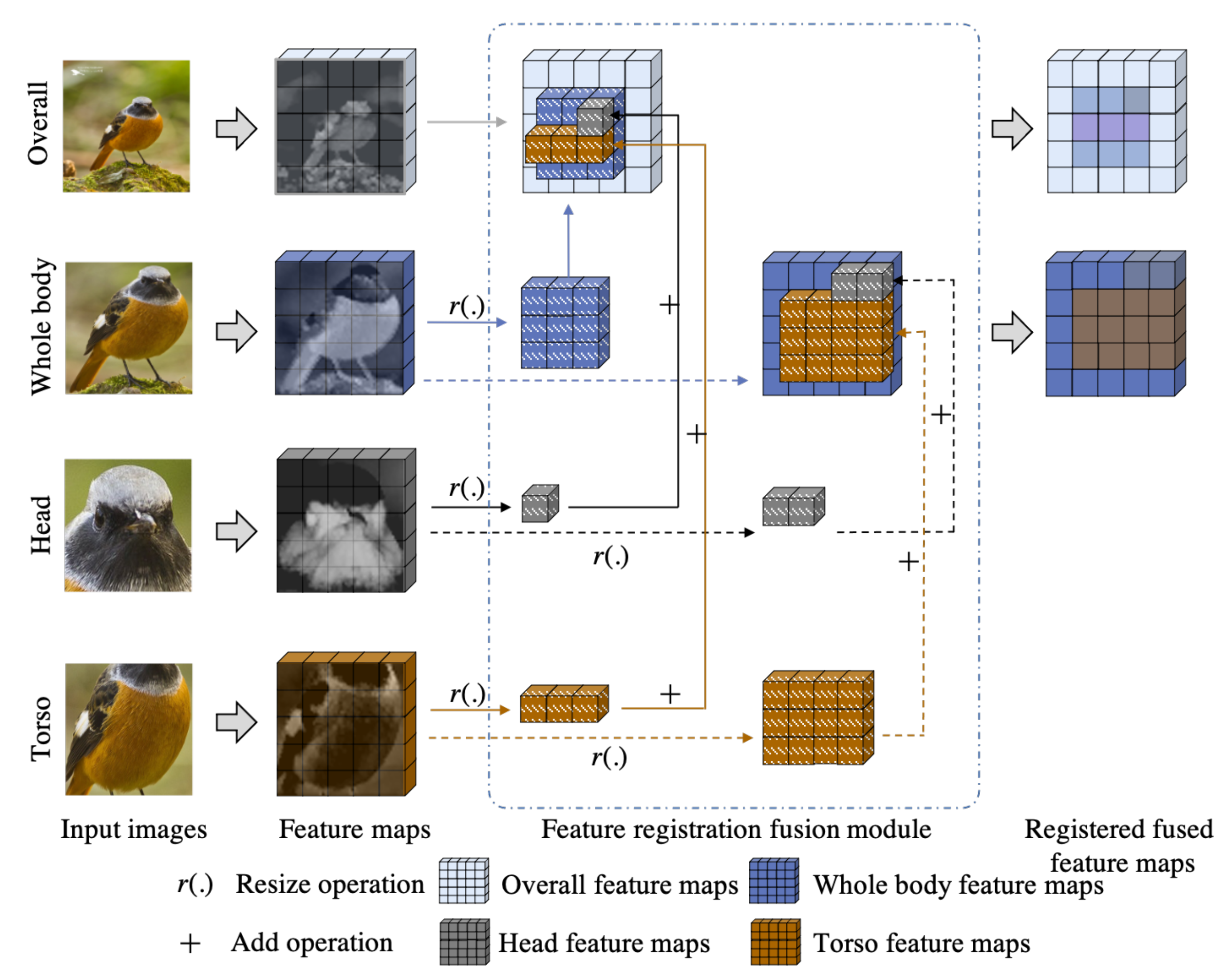
  • A mechanism of registration–fusion features calculates the dimension and location relationships between global (object) regions and local (parts) regions to generate the registration information and fuses the local features into the global features with registration information to generate the fine-grained feature.
  • The proposed method surpasses the state-of-the-art methods on the three popular datasets, including CUB200-2011, Stanford Cars, and FGVC-Aircraft datasets in both quantitative and qualitative evaluation.
The rest of this article is organized as follows. In Section 2, we introduce the proposed network, including the mechanism of registration–fusion features and the overall framework with the forward and backward propagations, for the fine-grained classification. Section 3 provides an evaluation of our OR-Net method against its state-of-the-art counterparts on three popular datasets. In Section 4, we present our conclusions.

2. Methodology

Object–part registration–fusion Net (OR-Net) comprises three streams, including overall stream, whole-body stream, and parts stream, and one registration–fusion feature module, as shown in Figure 2. In Figure 2, the overall and whole-body streams address the global information with different percentages of background, which are indicated as light blue and deep blue feature maps, respectively; they apply the registration–fusion feature module to obtain the fine-grained features. The parts streams handle the local information, which grabs from various object localization and provides the local feature for the registration–fusion module. The local information (feature maps), shown in Figure 2, from the part streams are indicated as gray and brown to present the parts information of torso and head. OR-Net extracts global and local features of the object from different CNN-streams and generates the feature maps by registering and fusing the global and local features generated from various CNN-streams on the overall stream and whole-body stream. Moreover, we consider the effects of various levels of streams to conduct the final classification. In the following sections, we first introduce the procedure of the registration–fusion feature module. Next, we present the architecture of OR-Net with forwarding and backward propagation. Finally, we present the algorithm of the proposed OR-Net to state the scientific methods and steps to achieve the presented results.

2.1. Feature Registration–Fusion Module

We take a bird as an example to explain the operation process of the proposed feature registration fusion module, which efficiently fuses the feature map from various resources, as shown in Figure 3. To execute the feature registration module procedure, we separate a bird into various components, including the bird’s head, the bird’s torso, the bird’s whole body, and the overall image. Then, we use benchmarked CNN with multi-stream to extract the feature maps, including the feature maps of the head, torso, the whole body, and overall and are indicated as gray, blue, navy blue, and light blue. Next, we consider the overall and the whole-body features as the registering targets and integrate the feature of each part into the overall and whole-body streams.
There are two main phases to complete the feature registration fusion module: (1) to calculate the ratio of size between the original image and its feature map, (2) to compute the registering location of each registered feature.
In the following description, we take the feature maps of the original stream as the registering target and the feature maps of the whole-body and parts stream as the registered features to describe the registration–fusion module’s procedure.
Firstly, we calculate the size’s ratio original image I , and its feature map f γ = { o s } , to be expressed as,
[ r w γ = { o s } , r h γ = { o s } ] = [ w f γ = { o s } w I , h f γ = { o s } h I ]
where w and h are the width and height of the image or the feature map, r w and r h are the ratio of width and height between original image ( I ) and its feature map ( f γ = { o s } ). Next, we resize the feature maps of each stream and express the equation definition as follows,
f γ = R ( f γ , w f γ , h f γ ) , γ = { w s , p s }
where f γ is the resized feature map, R ( . ) is the resize function, w f γ and h f γ are the width and height of f γ , and γ = { w s , p s } . In this study, we take bilinear interpolation as the resize function. Then, we calculate the width ( w f γ ) and height ( h f γ ) of the resized feature map with the following equation,
[ w f γ , h f γ ] = [ w I γ × r w , h I γ × r h ] , γ = { w s , p s }
where w I γ and h I γ are the width and height of sub-images which are cropped from the original image. We operate the ceiling operation to calculate the height and width of the resized feature map to avoid the problem of the width and height becoming 0 after resizing.
Moreover, coordinate information of the resized feature is needed to register the resized features f γ = w s , p s into the feature map of the registering target, which are generated from the original stream f γ = o s . Therefore, we re-calculate the coordinates of each resized feature map according to their original coordinates in the original image I , which can be expressed as,
[ C x γ , C y γ ] = [ C x γ × r w , C y γ × r h ] , γ = { w s , p s }
where C x γ and C y γ are the new coordinates of x and y axes after resize, and C x γ and C y γ are the coordinates of x and y axes of sub-images in the original image. We operate the floor operation to calculate the new coordinates of the x and y axes to avoid the problem where the position coordinate value exceeds the range of the original image.
Finally, we add the resized features ( f γ = w s , p s ) into the target’s feature map, which are generated from the original stream ( f γ = o s ) according to the new coordinate.

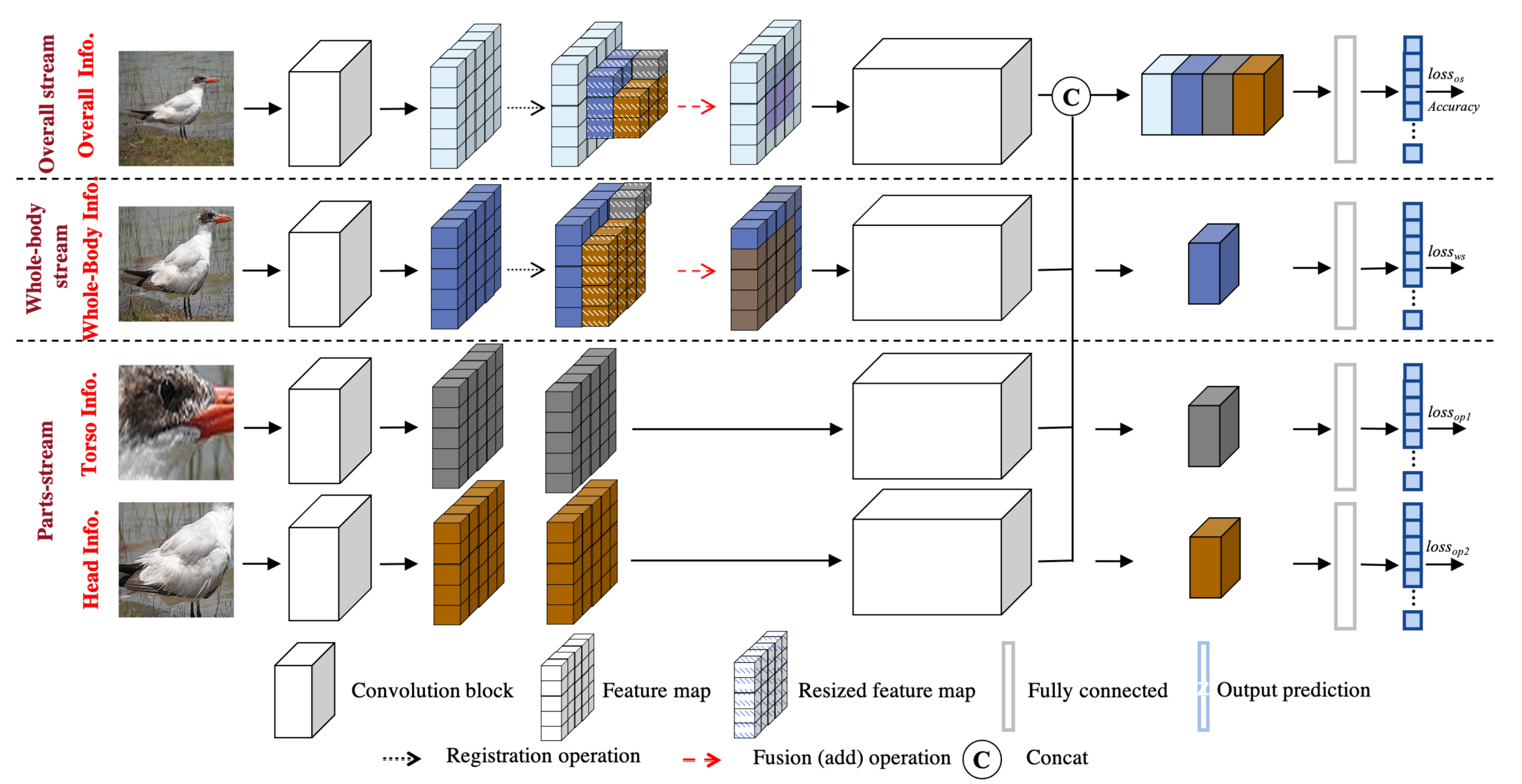
2.2. Network Architecture

Information fusion, which integrates the characteristics from various resources, plays a significant function in various computer vision topics. To effectively integrate the features, we designed the OR-Net, which contains multiple CNN streams and one registration–fusion features module, as shown in Figure 2. In Figure 2, each stream has several convolution blocks in which the registration–fusion features module is embedded in the original stream and whole-body stream, and each convolution block has several convolution operations. Specifically, we took the original image (overall image) as the input of the original stream, the whole-body image of the bird as the input of the whole-body stream, and the bird’s head and the bird’s torso are the inputs of two parts-streams. The first convolution blocks of each stream can be expressed as follows:
O γ m = 1 = { f γ n 1 } = F ( s γ , W γ n 1 , b γ n 1 ) , γ = { o s , w s , p s } , n 1 N
where O γ m = 1 , γ = { o s , w s , p s } is the output of the first convolution block of each stream and is taken as the input for the registration–fusion features module and the next convolution block of each stream; m is the number of convolution blocks in the network; f γ n 1 O γ m = 1 are the feature maps after operating first convolution block and n 1 N is the number of feature maps; F is convolution operation which is used to extract features by using convolution operator; s γ , γ = { o s , w s , p s } are the sub-images of the original image including the bird’s overall image, bird’s whole-body image, and the bird’s parts (head and torso); and W γ n 1 and b γ n 1 are the weight kernel and the bias of F (.), respectively. Next, the registration–fusion features module, which is embedded on the original stream and whole-body stream, receives the features from the first convolution blocks of each stream and generates the registration–fusion feature maps for the second convolution block. The output of the second convolution block on the overall stream and the whole-body stream is expressed as follows:
O γ = { o s , w s } m = 2 = { f γ = { o s , w s } n 2 } = F ( f r , W γ = { o s , w s } n 2 , b γ = { o s , w s } n 2 ) , n 2 N
where O γ = { o s , w s } m = 2 is the output of the second convolution block using the registered and fused feature maps from the registration–fusion feature module on the original stream and the whole-body stream; f γ = { o s , w s } n 2 O γ = { o s , w s } m = 2 are the feature maps, which are generated from registration–fusion feature maps, and n 2 N is the number of the feature maps on the second convolution block; W γ = { o s , w s } n 2 , b γ = { o s , w s } n 2 are the weight kernel and the bias of F (.), respectively, and can be operated on the registered feature maps; f r is the set of the registration–fusion feature maps and is expressed as,
f r = F ( f γ i , I γ i ) | γ { o s , w s , p s }
where F ( . ) is the registration–fusion feature function that is used to generate the registration–fusion feature map. I γ i is the information set of the ith feature map, which includes the size of inputs and feature map, the size of parts images, and the coordinates of parts in the full image. f γ i is the ith feature map of the original stream, the whole-body stream, and parts streams. Next, we take O γ = p s m = 1 as the input into the second convolution block of the parts stream. The output is described as follows:
O γ m = 2 = { f γ n 2 } = F ( Ψ 1 , W γ n 2 , b γ n 2 )
where O γ m = 2 , γ = { p s } is the output of the second convolution block of the parts stream and are taken as the input for next convolution block; f γ n 2 O γ m = 2 is the feature maps and n 2 N is the number of feature maps; Ψ = { O γ = p s m = 1 } is the input of the second convolution block for the parts-stream; and W γ n 2 and b γ n 2 are the weight kernel and the bias of F (.), respectively. Then, we take O γ m = 2 , γ = { o s , w s , p s } as the input for the next convolution block of the respective stream. The output is described as follows:
O γ m = 3 = { f γ n 3 } = F ( Ψ 2 , W γ n 3 , b γ n 3 )
where O γ m = 3 , γ = { o s , w s , p s } is the output of the third convolution block of the original, the whole-body, and parts streams and are taken as the input for next convolution block of the respective stream; f γ n 3 O γ m = 3 are the feature maps and n 3 N is the number of feature maps; Ψ 2 = { O γ = o s m = 2 O γ = w s m = 2 , O γ = p s m = 2 } are the inputs of the third convolution block for registering-stream, object-stream, and parts-stream, respectively; and W γ n 3 and b γ n 3 are the weight kernel and the bias of F (.), respectively. Next, we take O γ m = 3 , γ = { o s , w s , p s } as the input for the last convolution block of the respective stream. The output is described as follows:
O γ m = 4 = { f γ n 4 } = F ( Ψ 3 , W γ n 4 , b γ n 4 )
where O γ m = 4 , γ = { o s , w s , p s } is the output of the fourth convolution block of the original, the whole-body, and parts streams and are taken as the input for the fully connected layers; f γ n 4 O γ m = 4 are the feature maps and n 4 N is the number of feature maps; Ψ 3 = { O γ = o s m = 3 , O γ = w s m = 3 , O γ = p s m = 3 } are the inputs of the third convolution block for original stream, the whole-body stream, and parts stream, respectively; and W γ n 4 and b γ n 4 are the weight kernel and the bias of F (.), respectively. Finally, we applied the fully connected layers for each stream and used that output to fine-grain identification, represented as follows:
O γ f c = F γ f c ( Ψ f c , W γ f c , b γ f c ) , γ = { o s , w s , p s }
C γ = F s ( O γ f c ) , γ = { o s , w s , p s }
where O γ f c , γ = { o s , w s , p s } is the output of the original, the whole-body, and parts streams after operating the fully connected operation ( F f c ); F f c is the operation with three fully connected layers; Ψ f c = { ψ γ } , γ = { o s , w s , p s } in which ψ γ = o s = C γ = o s f c , ψ γ = w s = O γ = w s m = 4 , and ψ γ = p s = O γ = p s m = 4 ; C γ = o s f c is the operation of concatenation in the original stream and corresponds to C γ = o s f c = [ O γ = o s m = 4 , O γ = w s m = 4 , O γ = p s m = 4 ] ; W γ f c and b γ f c are the weight kernel and the bias of F f c (.), respectively. C γ = o s , C γ = w s , C γ = p s are the probability vector of the fine-grained classification result of the original, the whole-body, and parts streams, respectively, after executing the softmax operation ( F s ). Then, we take the result of the original stream as the finial classification result.
The networking procedure of each stream is summarized in the following series of formulas.
O γ f c = Ψ f c W γ f c + b γ f c = ( O γ m = 3 W γ 4 + b γ 4 ) W γ f c + b γ f c = ( ( O γ m = 2 W γ 3 + b γ 3 ) W γ 4 + b γ 4 ) W γ f c + b γ f c = ( ( ( O γ m = 1 W γ 2 + b γ 2 ) W γ 3 + b γ 3 ) W γ 4 + b γ 4 ) W γ f c + b γ f c
We take the equation of cross-entropy to calculate the loss between the ground truth and the classification results as expressed as follows:
L γ = i = 1 M j = 1 N T i , j · l o g ( C γ i , j ) , γ = { o s , w s , p s }
where T is the ground truth of a one-hot vector; T i , j is the ground truth of the ith class at the jth image; L γ = o s , L γ = w s , L γ = p s are the total loss of the original, the whole-body, and parts streams, respectively; N is the number of classes; and M is the number of testing images. The total loss is expressed as follows,
L t o t a l = i = 1 M ( γ ) L γ , γ = { o s , w s , p s }
where L t o t a l is the total loss and is the summation of L γ = o s , L γ = w s , and L γ = p s ; and M ( γ ) is the number of loss. Then, we adjust the framework of the network using the loss value to update the weights of the network in the procedure of the backpropagation, which can be described as follows:
m t = β m t 1 + L t o t a l W γ l r
where m is the momentum, β is the decay coefficient of the momentum, t is the number of the current iteration, t + 1 is the number of the next iteration, and W γ is the weight of the γ { o s , w s , p s } component. Next, we elaborate on the backpropagation procedure of the second convolution block, which considers the information for feature registration, to explain its function from the mathematical model. The forward propagation formula of the original stream at the second block can be rewritten as follows:
O γ = o s m = 2 = W γ = o s n 1 f r + b γ = o s n = 2
where f r corresponds to the registration–fusion feature maps which is the summation by adding feature maps of the whole-body and parts streams into the original stream and can be rewritten as:
O γ = o s m = 2 = W γ = o s n 1 ( f γ = o s + f γ = w s + f γ = p s ) + b γ = o s n = 2
Its backward propagation for updating the weights can be expressed as follows:
L t o t a l W γ = o s n = 2 = L t o t a l f r × f r W γ = o s n = 2 = L t o t a l f r × f γ = o s + L t o t a l f r × ( f γ = w s + f γ = p s )
In Equation (19), the weight adjustment of the overall stream not only considers the information of overall images but the information of the whole-body and parts streams. The forward and backward propagation in the whole-body stream is similar to the overall stream but only takes features from the parts steam into the registration–fusion feature module.

2.3. Procedure of the Proposed OR-Net

We demonstrate the procedure of the proposed object–part registration–fusion Net (OR-Net) in Algorithm 1 to state the scientific methods and steps which are used to achieve the presented results. In Algorithm 1, we take three materials as the input in the process of OR-Net: (1) the resource images, (2) the coordinates of parts in the original image, (3) the number of iterations. Specifically, we resize the original image I, the parts’ images I γ = { w s , p s } into 224 × 224 and take as the input images into overall, whole-body and parts streams. Moreover, we also need the information of each part’s coordinates, C x γ , y γ and γ = { w s , p s } , in the original image and the size of the original image [ w I , h I ] to complete the procedure of generating the registration–fusion features. In addition, we set the iteration number as N when training. The output of the OR-Net is the birds’ categories Y.
In the forward training procedure, for each iteration, we first resize each input image into 224 × 224 and extract the feaures from each CNN stream after the first convolution block, f γ = o s , w e , p s b i , 1 , where b i , 1 is the 1st convolution block with i number of feature maps. Next, we generate the registration–fusion features using f r function in overall and whole-body streams. Then, we execute the rest of the convolution blocks in the CNN to generate the final feature maps O γ = { o s , w s , p s } and operate the fully connected operation to generate the features O γ = o s f c for classification. Finally, we obtain the predicted results Y by operating softmax operation for O γ = o s f c .
In the backward training procedure, we separately calculate the L o s s γ = { o s , w s , p s } for each stream and summarize each loss to generate the total loss, L o s s t o t a l , for adjusting the network.
Algorithm 1: An algorithm of the proposed object–part registration–fusion Net (OR-Net).
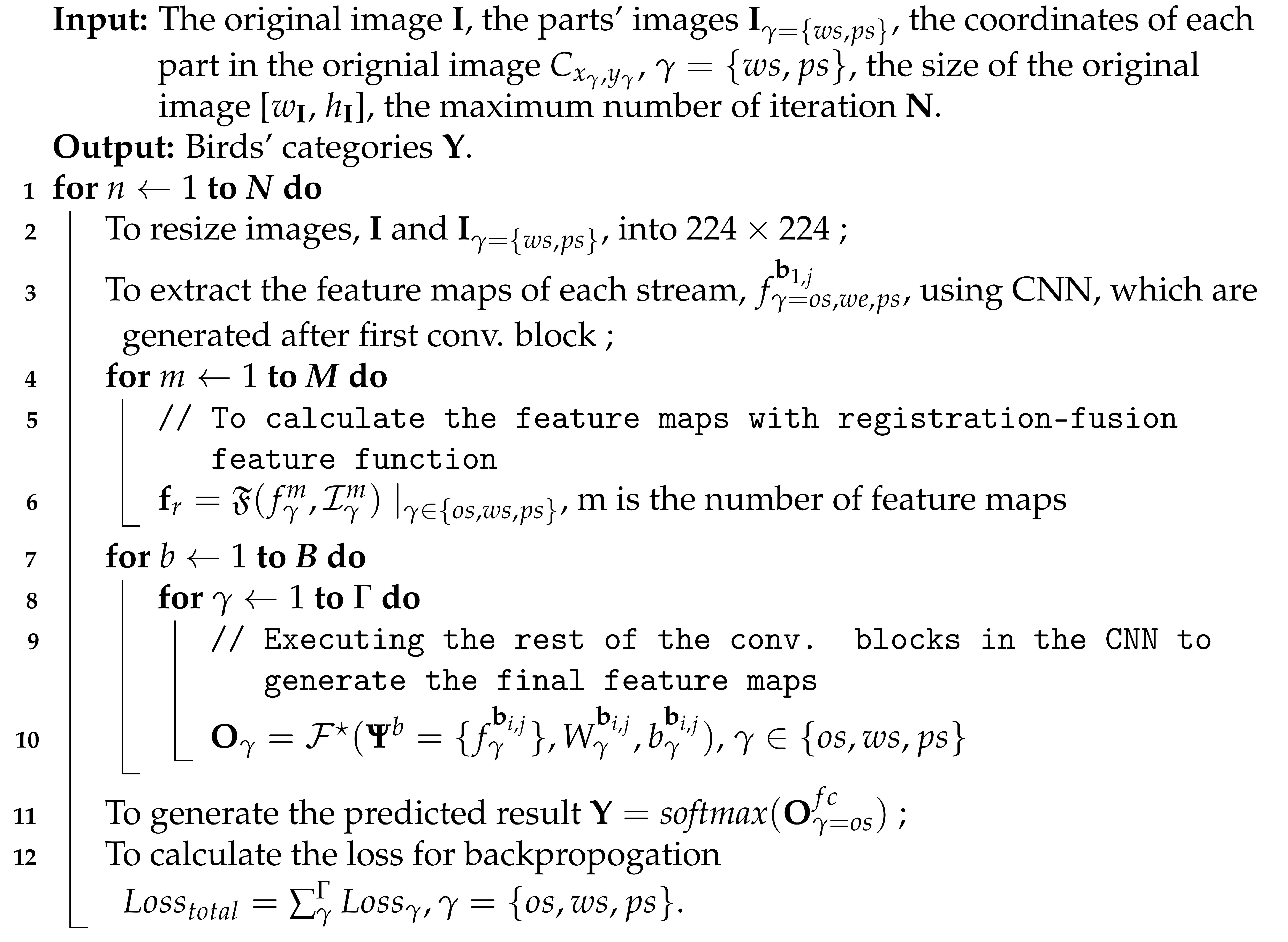
Symmetry 13 01838 i001

3. Experiment

In this section, we first present the datasets and their benchmarks used in the performance evaluation. Next, we examine the diagnostic and ablation experiments to demonstrate the effectiveness of the proposed framework. Finally, we compare our algorithm with state-of-the-art approaches with the quantitative and qualitative evaluation to demonstrate the performance.

3.1. Experimental Datasets and Implementation Details

In this work, we take three challenging fine-grained image classification datasets, including Caltech-UCSD Birds (CUB-200-2011) [21], Stanford Cars [22], and FGVC Aircraft [23], which are widely used for fine-grained image classification, to evaluate the performance of our algorithm. CUB-200-2011 contains 200 categories and has 11,788 images (5994/5794 images for training/testing), Stanford Cars has 196 types of cars and contains 16,185 images (8144/8041 images for training/testing), and FGVC Aircraft owns 100 classes with 10,000 images (6667/3333 images for training/testing). These datasets collect a large number of images with various targets. They provide the label of each image and the bounding box of the target in each image, but the bounding boxes of each part of the object are lost. Therefore, we add the parts’ bounding boxes of each object for the following experiments. All part rectangles of birds, aircraft, and cars are manually located and cropped except the part rectangles of birds on the CUB200-2011 dataset. We use the part annotations (key points) of the bird to identify and cut each part with rectangles [24].
In the implementation details, we generate the classifier using two NVIDIA GTX1080Ti (11G) GPU and symmetrically operating the algorithm with mini-batch = 8 for each GPU on the Ubuntu16.04 system with TensorFlow 1.12. We take Momentum SGD as the optimizer with an initial learning rate 1 e 2 and use the cosine decay function to decay the learning rate when training. Moreover, we use Relu and cross-entropy as the active and loss functions, respectively, and set 100 epochs in the training process. In addition, we take densenet-121 as the backbone, which is pre-trained on ImageNet [25], and size the image into 224 × 224 for each stream.

3.2. Diagnostic and Ablation Experiments

In this subsection, we execute diagnostic and ablation experiments to present the feasibility and effectiveness of the proposed network on the CUB200-2011 dataset.

3.2.1. Diagnostic Experiments

In the diagnostic experiments, we design significance testing to prove the significance of the proposed registration–fusion feature strategy.
Significance testing: The feature registration and fusion function are the keys of the proposed object–parts registration–fusion Net (OR-Net). Therefore, we execute the paired-samples T-test as the significance testing to verify the prominence of the feature-registration module with two testing plans (I and II) on these three datasets. The plan I is the scenario with four streams, including the overall stream, the whole-body stream, and two parts streams, and plan II is with two streams, including the overall and the whole-body streams. In the significance testing, we take densenet121 as the backbones to experiment with 5-fold cross-validation and use SPSS statistics software in executing the paired-samples T-test to realize the significance level for each plan, as shown in Table 1.
In Table 1, the varibles of X, Y, “Sig. ( 2-tailed)”, and Δ refer to the proposed network (with the registration–fusion feature module), the standard network (without the registration–fusion feature module), the P-value of the two-sided significance (significance), and the difference between X and Y for each fold cross-validation. In Table 1, the proposed framework (X) accuracies are higher than the standard network (Y) in every fold experiment, either in plan I or plan II on three datasets. Moreover, their significant p-values (Sig.) are all less than 0.05 in the plan I and II on all three datasets. The paired-samples T-test shows that the model with the registration–fusion feature module has significant performance, proving the proposed module can efficiently increase the accuracy.

3.2.2. Ablation Experiments

In this subsection, we design two ablation experiments to demonstrate the performance of the proposed OR-Net: (1) registering objectives and (2) registering position.
Registering objectives: We design four scenarios with Top-1 accuracy: (I) non-registering (none), (II) overall stream (OS), (III) whole-body stream (WS), and (IV) overall + whole-body streams (OS + WS) to demonstrate the effects of using various registering objectives, as shown in Table 2. The basic framework of each scenario is OR-Net without the registration–fusion feature module. Scenario I does not have the registration–fusion feature model; scenario II considers the registration–fusion feature model into the overall stream (OS); scenario III takes the registration–fusion feature model into the whole-body stream (WS); scenario IV considers the registration–fusion feature model into the overall stream (OS) and whole-body stream(WS). In Table 2, the scenario I has the lowest accuracy and is 87.2%. Scenario II and III consider the registration–fusion feature module, and both achieve 87.5%, which is 0.3% higher than the scenario I. In Scenario IV, we simultaneously utilize the registration–fusion feature module into overall + whole-body streams; it has the highest accuracy and achieves 87.7%, and is 0.5% higher than the network without using the registration–fusion feature module.
The analysis of the registering objectives proves that the multi-parts feature-registration module is helpful to improve the classification accuracy, and the best combination is to execute the feature-registration module on the overall and whole-body stream.
Registering position: We operated the feature-registration module at various positions in the network to find out the best position in the network, and the analysis results are shown in Table 3. Conv.-1 refers to the registration–fusion feature module operated after the first convolution operation, which is on the backbone (Densenet-121); DB-1, DB-2, DB-3, and DB-4 refer to the operation of feature registering which occurred after operating the dense block 1, 2, 3, and 4, respectively. In Table 3, the best Top-1 accuracy occurs at DB-1, which has the 56 × 56 size of feature maps. The features obtained after operating dense block 1 have shallow features, and the size is suitable for registering and fusing.

3.3. Experimential Analysis on the Popular Datasets

To illustrate the performance of the proposed framework, we examine the proposed algorithm with the state-of-the-art methods on the popular datasets, including CUB200-2011, Stanford Cars, and FGVC Aircraft datasets. Moreover, we demonstrate the comparison results with the quantitative and qualitative forms to present the robustness of the proposed network.

3.3.1. Quantitative Evaluation

In each quantitative result, we present the compared methods with information on the source, year, training phase, testing phase, model, dimension, size, and accuracy. Source refers to the publication information of the article in which [C] and [J] refer to conference and journal articles. Year refers to the published year of the articles. The model refers to the type of convolutional network (backbone) used in those articles; dimension is the size of the fully connected layer of each method; size is the input size of each method; and accuracy presents the classification results of each method. The symbol “-” presents the lost information, which cannot be found in the manuscript, and the released code of the method.
We quantitatively compare the proposed approach with the 27 popular methods, which are published in the famous international conferences or international journals from 2014 to 2020, on the CUB200-2011, Stanford Cars, and FGVC Aircraft datasets as shown in Table 4. In Table 4, we divide the table into two parts with a thick solid line: the upper part is the comparison object whose input image size is nearly 224, and the bottom half is the comparison object whose input image size is approximately 448, and demonstrate our results in the last row of the table. Moreover, we indicate the accuracy with red color when the method has the highest accuracy with size 224 × 224 , indicating the accuracy with bold when the method has the highest accuracy with size 448 × 448 , and indicating the accuracy with bold red color when the method has the highest accuracy with both sizes 224 × 224 and 448 × 448 .
For experiments in the CUB200-2011 dataset, the performance of the proposed method achieves 87.7% accuracy. It has the best accuracy compared to the other methods, uses images with 224 × 224 size, and is 0.2% higher than the second-best approach, NTS. Moreover, the dimension of the NTS is 2.5 times larger than the OR-Net. To compare with the methods that use BBox and parts’ information, OR-Net has the best accuracy and is 0.4% higher than the second-best approach, Mask-CNN; its usage of image sizes and dimensions are 0.5 and 1/3 times than Mask-CNN, respectively. Although iSQRT-COV and DCL have the best and second-best accuracy on the CUB200-2011 dataset and achieve 88.7% and 87.8%, respectively, the OR-Net has the third-best accuracy, and its input size is 224 × 224 , which is 0.5 times smaller than iSQRT-COV and DCL. In addition, OR-Net has a small dimension and is 1/8 times smaller than iSQRT-COV.
To compare with state-of-the-art methods on the Stanford Cars dataset, OR-Net has the best accuracy and achieves 94.5%; it is 0.6% higher than the second-best approaches, NTS and GSFL-Net, in which the input sizes of NTS and GSFL-Net are 224 × 224 and 448 × 448, respectively. Moreover, the dimension of OR-Net is 0.4 and 0.32 times smaller than the second-best approaches, NTS and GSFL-Net, respectively. To compare with the methods which use the information of BBox and parts, OR-Net has the best accuracy and is 2.0% and 3.2% higher than the second-best and third-best approaches, MDTP and FCAN, respectively; its input size is 0.5 times smaller than second-best and third-best approaches.
Finally, we demonstrate the quantitative comparison results of each method on the FGVC Aircraft dataset. The proposed OR-Net has the best accuracy compared to thirteen state-of-the-art methods and achieves 93.8%; it is 0.8% and 2.4% higher than the second-best and third-best methods, DCL, iSQRT-COV, and NTS, respectively; its input size is 0.5 times smaller than the second-best and third-best approaches. Although OR-Net’s dimension is two times larger than the second-best approach, DCL, it is 0.4 and 0.13 times than the third-best approaches, iSQRT-COV, and NTS.
All in all, the proposed method is the best approach comparing with the state-of-the-art methods, which use the input size of 224 × 224 on each popular dataset, and its dimension is smaller than most of the compared methods.

3.3.2. Qualitative Evaluation

We demonstrate the qualitative results in Table 5 and Table 6 to present the registration–fusion features and to validate the effectiveness and superiority of the proposed method.
In Table 5, we present three sets of images for each analyzed target, including bird, car, and aircraft. The overall, whole-body, torso, and head information (info.) are used to classify bird species; the overall, whole-body, side, and back (rear) information are considered in the classification of the car; overall, whole-body, head, and back (rear) are for aircraft. Furthermore, we demonstrate the feature maps of each information selected from a set of feature maps of each stream with the best performance after operating the first dense block. In Table 5, the characteristics of the bird are not apparent on the feature which is generated from the overall image, but they are obvious on the features which are extracted from the whole-body, torso, and head images, especially torso and head. The characteristics of the head and the torso are around the eyes and on the wings (input image), and they are concentrated in the area with high brightness (feature image). The registering feature integrates the features from the various streams that can enhance the characteristics of a bird (registering feature) and effectively improve the classification accuracy. In the Stanford Cars dataset, we select a car image with a front-side view to present the characteristics of a car. Although the features extracted from the overall and back images are not obvious, the features extracted from the whole-body and side images are obvious. The distinctive features, which are extracted from the full-body and side images, can make up for the insufficient discrimination of features which are extracted from the overall image. In the FGVC Aircraft dataset, we take an aircraft image with a side view as an example to present the difference of each feature generated from various streams. The feature generated by the overall image is only evident on the upper half of the fuselage, but the features from the rest of the streams are apparent. Therefore, the feature generated by the registration–fusion feature module is noticeable compared with the feature generated by the overall image.
In Table 6, we demonstrate the heatmaps of the proposed method (OR-Net) and the backbone (DenseNet-121) on CUB200-2011, Stanford Cars, and FGVC Aircraft datasets to present the effectiveness of the proposed framework, where “RF” refers to the proposed registration–fusion feature module and “DB” is the dense block. In Table 6, the blue color indicates that the model has less attention on this region, and the red color indicates that the model focuses on this region. In other words, the darker the color is, the more attention the model gives to this region. To present the difference between OR-Net and DenseNet-121, we use the same input for OR-Net and DenseNet-121 and randomly select a feature map from each block to generate its heatmap. In the CUB 200-2011 dataset, although these methods focus on the different parts of a bird, such as the bird’s head and the torso of a bird, on an image after executing the first dense bloc, the attention is low. The OR-Net uses the registration–fusion feature module, which assembles the feature from various parts of a bird, to increase the energy of the attention on a bird and significantly increases the attention to a bird compared to the heatmap of BD-1. The OR-Net gradually focuses on the whole body of a bird by sequentially executing convolution blocks 2,3,4 and has great attention compared to DenseNet-121. Although DenseNet-121 gradually concentrates the attention, the attention is around the bird, which is lower than OR-Net. In the Stanford Cars, OR-Net focuses on most car parts, and DenseNet-121 only focuses on a small part of the car after executing the first dense block. OR-Net has the registration–fusion feature module, which puts more attention on the car, making the subsequent modules focus more and more on the car. In contrast, most of the DenseNet-121 attention is on the background outside the car, and only less attention is on a small part of the car after executing the first dense block. Therefore, the successor modules of the first module of DenseNet-121 pay more and more attention to the outside area of the car. In the FGVC Aircraft, OR-Net and DenseNet-121 focus on most aircraft parts after executing the first dense block, but their attention level to the aircraft is different in the following dense blocks. OR-Net has the registration–fusion feature module, which assembles each part’s feature, making the following dense blocks pay more attention to the aircraft. Compared to the heatmap of OR-Net and DenseNet-121 on the last dense block, the OR-Net pays more attention to the aircraft than DenseNet-121.
In summary, the OR-Net considers the characteristics of different parts of an object, and various parts have been integrated at the early stages of the framework that allows the succeeding blocks in the network to further focus on the characteristics of an object.

3.3.3. Qualitative Analysis with Benchmarked Model

We analyze the performance of the benchmarked model (DenseNet-121) with various input information on the CUB200-2011 dataset and demonstrate the qualitative results in Table 7. In Table 7, the performance of the benchmarked model with a single resource, such as overall (original), whole-body, head, and torso images, is poorer than simultaneously considering all information. The highest Top-1 accuracy of the benchmarked model with a single resource is 83.4%, which is 0.38% lower than the benchmarked model with all information. However, the performance of the benchmarked model with all information is 0.5% lower than the proposed OR-Net.

4. Conclusions

This study proposed a novel convolutional neural network, object–part registration–fusion convolutional neural network (OR-Net), for fine-grained image classification. OR-Net contains multi-streams, including overall stream, whole-body stream, and parts stream. The whole-body stream and parts stream indicate the unique parts of the object, and their inputs are grabbed from the original image to provide more details when extracting features. The registration–fusion feature module integrates various features, such as whole-body information, parts information of the object, and overall information that contains large background, to increase the discrimination of the feature and pay more attention to the interesting object. The registration–fusion feature module considers the ratio of feature size between various features of parts used to register and fuse the information of each feature.
In the experiments, we compare the performance of the OR-Net with the state-of-the-art methods on three widely used datasets, Caltech-UCSD Birds (CUB200-2011), Stanford Cars, and FGVC Aircraft, and demonstrate the results with quantitative and qualitative evaluation. In quantitative evaluation, the proposed OR-Net has the best performance in classifying bird species with an input size of 224 × 224 and achieves 87.7%; it has the best accuracy in classifying car and aircraft types with various input sizes and achieves 94.5% and 93.8%, respectively. Moreover, OR-Net has a small dimension compared to the popular approaches. All in all, OR-Net performs well in quantitative and qualitative evaluation. The visualization shows that the proposed registration–fusion feature module provides the discriminative feature and makes the network pay more attention to the interesting target.

Author Contributions

Conceptualization, C.-W.L.; methodology, C.-W.L.; validation, C.-W.L. and M.L.; investigation, C.-W.L. and M.L.; writing—original draft preparation, C.-W.L.; writing—review and editing, C.-W.L. and J.L. All authors have read and agreed to the published version of the manuscript.

Funding

This research was funded by the China Postdoctoral Science Foundation under Grant 2018M632565, the Channel Postdoctoral Exchange Funding Scheme, and the Youth Program of Humanities and Social Sciences Foundation, Ministry of Education of China under Grant 18YJCZH093.

Data Availability Statement

Data available in a publicly accessible repository that does not issue DOIs. Publicly available datasets were analyzed in this study. The birds data can be found here: [Caltech-UCSD Birds-200-2011, http://www.vision.caltech.edu/visipedia/CUB-200-2011.html, accessed on 30 September 2021]. The cars data can be found here: [Stanford Cars, http://ai.stanford.edu/~jkrause/cars/car_dataset.html, accessed on 30 September 2021]. The aircrafts data can be found here: [FGVC Aircraft, https://www.robots.ox.ac.uk/~vgg/data/fgvc-aircraft/, accessed on 30 September 2021].

Conflicts of Interest

The authors declare no conflict of interest.

Abbreviations

The following abbreviations are used in this manuscript:
OR-NetObject-part registration-fusion Net
DCNNDeep Convolutional Neural Network

References

  1. Lin, C.W.; Ding, Q.; Tu, W.H.; Huang, J.H.; Liu, J.F. Fourier dense network to conduct plant classification using UAV-based optical images. IEEE Access 2019, 7, 17736–17749. [Google Scholar] [CrossRef]
  2. Qian, W.; Huang, Y.; Liu, Q.; Fan, W.; Sun, Z.; Dong, H.; Wan, F.; Qiao, X. UAV and a deep convolutional neural network for monitoring invasive alien plants in the wild. Comput. Electron. Agric. 2020, 174, 105519. [Google Scholar] [CrossRef]
  3. Hiary, H.; Saadeh, H.; Saadeh, M.; Yaqub, M. Flower classification using deep convolutional neural networks. IET Comput. Vis. 2018, 12, 855–862. [Google Scholar] [CrossRef]
  4. Bae, K.I.; Park, J.; Lee, J.; Lee, Y.; Lim, C. Flower classification with modified multimodal convolutional neural networks. Expert Syst. Appl. 2020, 159, 113455. [Google Scholar] [CrossRef]
  5. Hossain, M.S.; Al-Hammadi, M.; Muhammad, G. Automatic fruit classification using deep learning for industrial applications. IEEE Trans. Ind. Inform. 2018, 15, 1027–1034. [Google Scholar] [CrossRef]
  6. Steinbrener, J.; Posch, K.; Leitner, R. Hyperspectral fruit and vegetable classification using convolutional neural networks. Comput. Electron. Agric. 2019, 162, 364–372. [Google Scholar] [CrossRef]
  7. Obeso, A.M.; Benois-Pineau, J.; Acosta, A.Á.R.; Vázquez, M.S.G. Architectural style classification of Mexican historical buildings using deep convolutional neural networks and sparse features. J. Electron. Imaging 2016, 26, 011016. [Google Scholar] [CrossRef]
  8. Yi, Y.K.; Zhang, Y.; Myung, J. House style recognition using deep convolutional neural network. Autom. Constr. 2020, 118, 103307. [Google Scholar] [CrossRef]
  9. Lin, C.W.; Lin, M.; Yang, S. SOPNet Method for the Fine-Grained Measurement and Prediction of Precipitation Intensity Using Outdoor Surveillance Cameras. IEEE Access 2020, 8, 188813–188824. [Google Scholar] [CrossRef]
  10. Lin, C.W.; Yang, S. Geospatial-Temporal Convolutional Neural Network for Video-Based Precipitation Intensity Recognition. In Proceedings of the 2021 IEEE International Conference on Image Processing (ICIP), Anchorage, AK, USA, 19–22 September 2021; pp. 1119–1123. [Google Scholar]
  11. Wei, C.C.; Huang, T.H. Modular Neural Networks with Fully Convolutional Networks for Typhoon-Induced Short-Term Rainfall Predictions. Sensors 2021, 21, 4200. [Google Scholar] [CrossRef] [PubMed]
  12. Wei, C.C.; Hsieh, P.Y. Estimation of hourly rainfall during typhoons using radar mosaic-based convolutional neural networks. Remote Sens. 2020, 12, 896. [Google Scholar] [CrossRef] [Green Version]
  13. Branson, S.; Van Horn, G.; Belongie, S.; Perona, P. Bird species categorization using pose normalized deep convolutional nets. arXiv 2014, arXiv:1406.2952. [Google Scholar]
  14. Lin, T.Y.; RoyChowdhury, A.; Maji, S. Bilinear cnn models for fine-grained visual recognition. In Proceedings of the IEEE ICCV, Santiago, Chile, 13–16 December 2015; pp. 1449–1457. [Google Scholar]
  15. Feichtenhofer, C.; Pinz, A.; Zisserman, A. Convolutional two-stream network fusion for video action recognition. In Proceedings of the IEEE Conference on Computer Vision and Pattern Recognition, Las Vegas, NV, USA, 30 June–01 July 2016; pp. 1933–1941. [Google Scholar]
  16. Zheng, H.; Fu, J.; Mei, T.; Luo, J. Learning multi-attention convolutional neural network for fine-grained image recognition. In Proceedings of the IEEE ICCV, Venice, Italy, 22–29 October 2017; pp. 5209–5217. [Google Scholar]
  17. Wu, L.; Wang, Y.; Li, X.; Gao, J. Deep attention-based spatially recursive networks for fine-grained visual recognition. IEEE Trans. Cybern. 2018, 49, 1791–1802. [Google Scholar] [CrossRef] [PubMed]
  18. Chen, S.; Tan, X.; Wang, B.; Hu, X. Reverse Attention for Salient Object Detection. In Proceedings of the The European Conference on Computer Vision (ECCV), Munich, Germany, 8–14 September 2018. [Google Scholar]
  19. Zhao, B.; Wu, X.; Feng, J.; Peng, Q.; Yan, S. Diversified visual attention networks for fine-grained object classification. IEEE Trans. Multimed. 2017, 19, 1245–1256. [Google Scholar] [CrossRef] [Green Version]
  20. Peng, Y.; He, X.; Zhao, J. Object-part attention model for fine-grained image classification. IEEE Trans. Image Process. 2017, 27, 1487–1500. [Google Scholar] [CrossRef] [PubMed] [Green Version]
  21. Wah, C.; Branson, S.; Welinder, P.; Perona, P.; Belongie, S. The Caltech-UCSD Birds-200-2011 Dataset; Technical Report; California Institute of Technology: Pasadena, CA, USA, 2011. [Google Scholar]
  22. Krause, J.; Stark, M.; Deng, J.; Li, F.F. 3d object representations for fine-grained categorization. In Proceedings of the IEEE ICCV Workshops, Sydney, NSW, Australia, 2–8 December 2013; pp. 554–561. [Google Scholar]
  23. Maji, S.; Rahtu, E.; Kannala, J.; Blaschko, M.; Vedaldi, A. Fine-grained visual classification of aircraft. arXiv 2013, arXiv:1306.5151. [Google Scholar]
  24. Wei, X.S.; Xie, C.W.; Wu, J.; Shen, C. Mask-CNN: Localizing parts and selecting descriptors for fine-grained bird species categorization. Pattern Recognit. 2018, 76, 704–714. [Google Scholar] [CrossRef]
  25. Deng, J.; Dong, W.; Socher, R.; Li, L.J.; Li, K.; Li, F.F. Imagenet: A large-scale hierarchical image database. In Proceedings of the IEEE CVPR, Miami, FL, USA, 20–25 June 2009; pp. 248–255. [Google Scholar]
  26. Zhang, N.; Donahue, J.; Girshick, R.; Darrell, T. Part-Based R-CNNs for Fine-Grained Category Detection. In European Conference on Computer Vision; Springer: Zurich, Switzerland, 2014; pp. 834–849. [Google Scholar]
  27. Lin, D.; Shen, X.; Lu, C.; Jia, J. Deep lac: Deep localization, alignment and classification for fine-grained recognition. In Proceedings of the IEEE CVPR, Boston, MA, USA, 7–12 June 2015; pp. 1666–1674. [Google Scholar]
  28. Wang, D.; Shen, Z.; Shao, J.; Zhang, W.; Xue, X.; Zhang, Z. Multiple granularity descriptors for fine-grained categorization. In Proceedings of the IEEE ICCV, Santiago, Chile, 13–16 December 2015; pp. 2399–2406. [Google Scholar]
  29. Xiao, T.; Xu, Y.; Yang, K.; Zhang, J.; Peng, Y.; Zhang, Z. The application of two-level attention models in deep convolutional neural network for fine-grained image classification. In Proceedings of the IEEE CVPR, Boston, MA, USA, 7–12 June 2015; pp. 842–850. [Google Scholar]
  30. Zhou, F.; Lin, Y. Fine-grained image classification by exploring bipartite-graph labels. In Proceedings of the IEEE Conference on Computer Vision and Pattern Recognition, Las Vegas, NV, USA, 30 June–1 July 2016; pp. 1124–1133. [Google Scholar]
  31. Zhang, Y.; Wei, X.S.; Wu, J.; Cai, J.; Lu, J.; Nguyen, V.A.; Do, M.N. Weakly supervised fine-grained categorization with part-based image representation. IEEE Trans. Image Process. 2016, 25, 1713–1725. [Google Scholar] [CrossRef] [PubMed]
  32. Yang, Z.; Luo, T.; Wang, D.; Hu, Z.; Gao, J.; Wang, L. Learning to navigate for fine-grained classification. In Proceedings of the European Conference on Computer Vision (ECCV), Munich, Germany, 8–14 September 2018; pp. 420–435. [Google Scholar]
  33. Dubey, A.; Gupta, O.; Guo, P.; Raskar, R.; Farrell, R.; Naik, N. Pairwise confusion for fine-grained visual classification. In Proceedings of the European Conference on Computer Vision (ECCV), Munich, Germany, 8–14 September 2018; pp. 70–86. [Google Scholar]
  34. Zheng, H.; Fu, J.; Zha, Z.J.; Luo, J. Looking for the devil in the details: Learning trilinear attention sampling network for fine-grained image recognition. In Proceedings of the IEEE Conference on Computer Vision and Pattern Recognition, Long Beach, CA, USA, 16–20 June 2019; pp. 5012–5021. [Google Scholar]
  35. Huang, Z.; Li, Y. Interpretable and Accurate Fine-grained Recognition via Region Grouping. In Proceedings of the IEEE/CVF Conference on Computer Vision and Pattern Recognition (CVPR), Seattle, WA, USA, 13–19 June 2020. [Google Scholar]
  36. Jaderberg, M.; Simonyan, K.; Zisserman, A. Spatial transformer networks. Adv. Neural Inf. Process. Syst. 2015, 28, 2017–2025. [Google Scholar]
  37. Liu, X.; Xia, T.; Wang, J.; Lin, Y. Fully convolutional attention localization networks: Efficient attention localization for fine-grained recognition. arXiv 2016, arXiv:1603.06765. [Google Scholar]
  38. Huang, S.; Xu, Z.; Tao, D.; Zhang, Y. Part-stacked cnn for fine-grained visual categorization. In Proceedings of the IEEE CVPR, Las Vegas, NV, USA, 27–30 June 2016; pp. 1173–1182. [Google Scholar]
  39. Moghimi, M.; Belongie, S.J.; Saberian, M.J.; Yang, J.; Vasconcelos, N.; Li, L.J. Boosted Convolutional Neural Networks. In Proceedings of the the British Machine Vision Conference (BMVC), York, UK, 19–22 September 2016; pp. 24.1–24.13. [Google Scholar]
  40. Wang, Y.; Choi, J.; Morariu, V.; Davis, L.S. Mining discriminative triplets of patches for fine-grained classification. In Proceedings of the IEEE CVPR, Las Vegas, NV, USA, 27–30 June 2016; pp. 1163–1172. [Google Scholar]
  41. Li, Z.; Yang, Y.; Liu, X.; Zhou, F.; Wen, S.; Xu, W. Dynamic computational time for visual attention. In Proceedings of the IEEE International Conference on Computer Vision Workshops, Venice, Italy, 22–29 October 2017; pp. 1199–1209. [Google Scholar]
  42. Fu, J.; Zheng, H.; Mei, T. Look closer to see better: Recurrent attention convolutional neural network for fine-grained image recognition. In Proceedings of the IEEE CVPR, Honolulu, HI, USA, 21–26 July 2017; pp. 4438–4446. [Google Scholar]
  43. Cai, S.; Zuo, W.; Zhang, L. Higher-order integration of hierarchical convolutional activations for fine-grained visual categorization. In Proceedings of the IEEE ICCV, Venice, Italy, 22–29 October 2017; pp. 511–520. [Google Scholar]
  44. Wang, Y.; Morariu, V.I.; Davis, L.S. Learning a discriminative filter bank within a cnn for fine-grained recognition. In Proceedings of the IEEE Conference on Computer Vision and Pattern Recognition, Salt Lake City, UT, USA, 18–23 June 2018; pp. 4148–4157. [Google Scholar]
  45. Li, P.; Xie, J.; Wang, Q.; Gao, Z. Towards faster training of global covariance pooling networks by iterative matrix square root normalization. In Proceedings of the IEEE Conference on Computer Vision and Pattern Recognition, Salt Lake City, UT, USA, 18–23 June 2018; pp. 947–955. [Google Scholar]
  46. Xin, Q.; Lv, T.; Gao, H. Random Part Localization Model for Fine Grained Image Classification. In Proceedings of the IEEE ICIP, Taipei, Taiwan, 22–25 September 2019; pp. 420–424. [Google Scholar]
  47. Chen, Y.; Bai, Y.; Zhang, W.; Mei, T. Destruction and construction learning for fine-grained image recognition. In Proceedings of the IEEE Conference on Computer Vision and Pattern Recognition, Long Beach, CA, USA, 15–20 June 2019; pp. 5157–5166. [Google Scholar]
  48. Ji, R.; Wen, L.; Zhang, L.; Du, D.; Wu, Y.; Zhao, C.; Liu, X.; Huang, F. Attention convolutional binary neural tree for fine-grained visual categorization. In Proceedings of the IEEE/CVF Conference on Computer Vision and Pattern Recognition, Seattle, WA, USA, 13–19 June 2020; pp. 10468–10477. [Google Scholar]
  49. Li, X.; Monga, V. Group based deep shared feature learning for fine-grained image classification. In Proceedings of the the British Machine Vision Conference (BMVC), Cardiff, UK, 9–12 September 2019; pp. 143.1–143.13. [Google Scholar]
Figure 1. The examples of using registration–fusion feature modules on different objects. The first column represents the original images of a bird, a car, and an aircraft; the second column shows the heatmaps of the first column, which is without consideration of registration–fusion features; the third column demonstrates the heatmaps of the first column, which considers registration–fusion features.
Symmetry 13 01838 g001
Figure 2. Architecture of the proposed convolutional neural network.
Symmetry 13 01838 g002
Figure 3. Procedure of registering and fusing feature maps from various levels of sub-features.
Symmetry 13 01838 g003
Table 1. Results of 5-fold cross-validation with two plans on widely used datasets.
DatasetCUB200-2011Stanford CarsFGVC Aircraft
PlansIIIIIIIII
SampleX(%)Y(%) Δ (%)X(%)Y(%) Δ (%)X(%)Y(%) Δ (%)X(%)Y(%) Δ (%)X(%)Y(%) Δ (%)X(%)Y(%) Δ (%)
#Fold
189.6389.450.1886.7886.570.2195.8295.730.0994.4094.140.2693.7593.450.3091.5090.700.80
289.6389.320.3187.3486.910.4395.1695.060.1094.5294.080.4493.9593.250.7091.2091.000.20
389.2088.720.4886.3586.220.1395.5095.470.0394.4094.370.0394.0593.100.9590.8090.650.15
489.3289.240.0886.4486.100.3495.5795.350.2295.0994.710.3894.0093.650.3591.0590.650.40
590.4090.270.1387.5687.260.3095.4795.250.2294.7194.210.5094.7594.200.5591.9091.100.80
Sig.
(2-tailed)
0.0310.0060.0250.0180.0090.029
Table 2. Comparison of the proposed net with the different number of registering objectives on CUB200-2011.
Registering StreamNoneOSWSOS + WS
Accuracy (Top-1, %)87.287.587.587.7
Table 3. Comparison of OR-Net with various registering positions on the CUB200-2011 dataset.
Registering PositionConv.-1DB-1DB-2DB-3DB-4
Size of feature map112 × 11256 × 5628 × 2814 × 147 × 7
Accuracy (Top-1, %)86.887.787.287.486.9
Table 4. Quantitative comparison results on the popular datasets.
MethodYearSourceDimensionSizeAccuracy
CUB200-2011Stanford CarsFGVC-Aircraft
PB R-CNN [26]2014ECCV[C]12,288224 × 22482.0%--
Pose Normalized CNNs [13]2014CVPR[C]13,512-85.4%--
Deep-LAC [27]2015CVPR[C]12,288227 × 22780.3%--
MG-CNN [28]2015ICCV[C]12,288224 × 22483.0%-86.6%
Two-level Attention [29]2015CVPR[C]-224 × 22477.9%--
VGG-BGL m [30]2016CVPR[C]4096224 × 22480.4%90.5%-
Weakly Supervised FG [31]2016TIP[J]-224 × 22479.3%--
NTS [32]2018ECCV[C]10,240224 × 22487.5%93.9%91.4%
PC [33]2018ECCV[C]-224 × 22486.9%92.9%89.2%
TASN [34]2019CVPR[C]2048224 × 22487.0%93.8%-
Interp [35]2020CVPR[C]2048256 × 25687.3%--
ST-CNN [36]2015NIPS[C]4096448 × 44884.1%--
Bilinear CNN [14]2015ICCV[C]262,144448 × 44885.1%91.3%84.1%
FCAN [37]2016CVPR[C]1,536448 × 44884.3%91.3%-
Part-Stacked CNN [38]2016CVPR[C]4096454 × 454 +
227 × 227
76.6%--
Boost-CNN [39]2016BMVC[C]262,144448 × 44886.2%92.1%88.5%
MDTP [40]2016CVPR[C]4096500 × 500-92.5%88.4%
DT-RAM [41]2017ICCV[C]2048448 × 44886%93.1%-
RA-CNN [42]2017CVPR[C]4096448 × 448 +
224 × 224
85.3%92.5%-
HIHCA [43]2017ICCV[C]-448 × 44885.3%91.7%88.3%
Mask-CNN [24]2018PR[J]12,288448 × 44887.3%--
DFL [44]2018CVPR[C]2048448 × 44887.4%--
iSQRT-COV [45]2018CVPR[C]32,896448 × 44888.7%93.3%91.4%
RP-CNN [46]2019ICIP[C]4096448 × 448 +
224 × 224
84.5%93.0%89.9%
DCL [47]2019CVPR[C]2048448 × 44887.8%94.5%93.0%
ACNet [48]2020CVPR[C]8192448 × 44887.6%93.5%90.4%
GSFL-Net [49]2020BMVC[C]12,801448 × 44887.6%93.9%88.2%
Ours2021-4096224 × 22487.7%94.5%93.8%
Table 5. Example of registering features on the popular dataset.
DatasetCUB200-2011Stanford CarsFGVC Aircraft
InformationOverall Info.Whole-Body Info.Torso Info.Head Info.Overall Info.Whole-Body Info.Side Info.Back Info.Overall Info.Whole-body Info.Head Info.Back Info.
Visualization
Input images Symmetry 13 01838 i002 Symmetry 13 01838 i003 Symmetry 13 01838 i004 Symmetry 13 01838 i005 Symmetry 13 01838 i006 Symmetry 13 01838 i007 Symmetry 13 01838 i008 Symmetry 13 01838 i009 Symmetry 13 01838 i010 Symmetry 13 01838 i011 Symmetry 13 01838 i012 Symmetry 13 01838 i013
Feature maps Symmetry 13 01838 i014 Symmetry 13 01838 i015 Symmetry 13 01838 i016 Symmetry 13 01838 i017 Symmetry 13 01838 i018 Symmetry 13 01838 i019 Symmetry 13 01838 i020 Symmetry 13 01838 i021 Symmetry 13 01838 i022 Symmetry 13 01838 i023 Symmetry 13 01838 i024 Symmetry 13 01838 i025
Registering
feature maps
Symmetry 13 01838 i026 Symmetry 13 01838 i027 Symmetry 13 01838 i028
Table 6. Visualization with heatmap on the popular datasets.
DatasetModelOriginal ImageDB-1RFDB-2DB-3DB-4
CUB200-2011Ours Symmetry 13 01838 i029 Symmetry 13 01838 i030 Symmetry 13 01838 i031 Symmetry 13 01838 i032 Symmetry 13 01838 i033 Symmetry 13 01838 i034
DenseNet Symmetry 13 01838 i035 Symmetry 13 01838 i036 Symmetry 13 01838 i037 Symmetry 13 01838 i038 Symmetry 13 01838 i039
Stanford CarsOurs Symmetry 13 01838 i040 Symmetry 13 01838 i041 Symmetry 13 01838 i042 Symmetry 13 01838 i043 Symmetry 13 01838 i044 Symmetry 13 01838 i045
DenseNet Symmetry 13 01838 i046 Symmetry 13 01838 i047 Symmetry 13 01838 i048 Symmetry 13 01838 i049 Symmetry 13 01838 i050
FGVC AircraftOurs Symmetry 13 01838 i051 Symmetry 13 01838 i052 Symmetry 13 01838 i053 Symmetry 13 01838 i054 Symmetry 13 01838 i055 Symmetry 13 01838 i056
DenseNet Symmetry 13 01838 i057 Symmetry 13 01838 i058 Symmetry 13 01838 i059 Symmetry 13 01838 i060 Symmetry 13 01838 i061
Table 7. Quantitative comparison with benchmarked model.
Input InformationModelTop-1 (%)
OverallDenseNet-12176.7
Whole-bodyDenseNet-12183.4
HeadDenseNet-12176.6
TorsoDenseNet-12171.6
AllDenseNet-12187.2
AllOR-Net87.7
Publisher’s Note: MDPI stays neutral with regard to jurisdictional claims in published maps and institutional affiliations.

