Damage Function of a Quasi-Brittle Material, Damage Rate, Acceleration and Jerk during Uniaxial Compression: Model and Application to Analysis of Trabecular Bone Tissue Destruction

Abstract

A diversity of quasi-brittle materials can be observed in various engineering structures and natural objects (rocks, frozen soil, concrete, ceramics, bones, etc.). In order to predict the condition and safety of these objects, a large number of studies aimed at analyzing the strength of quasi-brittle materials has been conducted and presented in publications. However, at the modeling level, the problem of estimating the rate and acceleration of destruction of a quasi-brittle material under loading remains relevant. The purpose of the study was to substantiate the function of damage to a quasi-brittle material under uniaxial compression, determine the rate, acceleration and jerk of the damage process, and also to apply the results obtained to predicting the destruction of trabecular bone tissue. In accordance with the purpose of the study, the basic concepts of fracture mechanics and standard methods of mathematical modeling were used. The proposed model is based on the application of the previously obtained differentiable damage function without parameters. The results of the study are presented in the form of plots and analytical relations for computing the rate, acceleration and jerk of the damage process. Examples are given. The predicted peak of the combined effect of rate, acceleration and jerk of the damage process are found to be of practical interest as an additional criterion for destruction. The simulation results agree with the experimental data known from the available literature.

1. Introduction

1.1. Research Problem

There is a large class of natural and artificial materials that, under mechanical influences, exhibit to a greater or lesser extent the property of brittleness. Such quasi-brittle materials include rocks, concrete, ceramics, bones, etc. A variety of quasi-brittle materials can be observed in various engineering structures and natural objects. With a decrease in temperature and some other influences, initially non-brittle materials can become quasi-brittle [1]. To avoid catastrophes, it is necessary to continue studying the mechanical behavior of quasi-brittle materials under various influences. Depending on the physical and mechanical properties of the material and the effects on it, the appropriate experimental research methods and mathematical models were used. The main focus in this study was given to the substantiation of the damage function of a quasi-brittle material, modeling the kinetics of destruction during uniaxial compression on the example of trabecular bone tissue. Trabecular bone is a multifunctional tissue that maintains a dynamic balance of structure and functions through repeated cycles of remodeling and adaptation to changes in physical activity and physiological needs [2,3,4]. The structure and functions of the trabecular bone tissue have been studied for hundreds of years [5], but a number of problems remain relevant [6]. The relevance of the topic and the practical significance of the presented work are determined by the fact that the solution of this problem is necessary to improve the understanding of the structure and function of the trabecular bone tissue, which will contribute to a more accurate prediction of the risk of bone fractures [7].

Within the framework of the abovementioned problem, the main issue in the presented research was to determine the speed, acceleration and jerk of the process of damage to a quasi-brittle material on the example of trabecular bone tissue under uniaxial compression. An analytical solution to this problem is proposed, which is obtained by standard methods of mathematical modeling of mechanical systems and is based on the use of the damage function justified in [8]. In addition to [8], a more detailed analysis of the damage function was carried out, which allowed us to obtain new analytical relations for determining the rate and other characteristics of the damage process of a quasi-brittle material. A method of applying the obtained results to predict damage to the trabecular bone tissue during uniaxial compression is proposed. Verification of simulation results was performed using experimental data known from the available literature.

1.2. Damage Models of Quasi-Brittle Materials

The approach to modeling the accumulation of damage which is used in this work is focused on the application of the methodology of fracture mechanics. The main stages of the evolution of fracture mechanics, starting with the classical work of Griffith (1920), are reflected in [9]. The development of damage models involves the use of certain information about the material that makes up the simulated object; in this case, it is the trabecular bone tissue. The initial building materials of bones are organic and inorganic substances. A functioning bone contains water, mineral and organic substances [10]. Approximately 50% of the dry mass of a bone is accounted for by inorganic material in the form of hydroxyapatite, which, by nature of its mechanical properties, belongs to brittle materials, but is not identical to hydroxyapatite which is contained in rocks [11]. The effect of hydroxyapatite as a component of bones is manifested in the fact that the load displacement diagrams in the tests of trabecular tissue samples for compression are similar (but not identical) to the diagrams obtained in the tests of quasi-brittle rocks; the difference is due to the influence of organic components in the bone material [11]. Accordingly, the trabecular bone tissue is considered in the available literature as a quasi-brittle material [12,13,14], for modeling the state of which some rock models can be adapted [15].

Figure 1 shows typical stress–strain plots for the models of an ideal brittle material and a quasi-brittle material. The diagram in Figure 1a is typical for ultra-high-strength concrete [16]. For a sufficiently small segment, the dependence is almost linear (Figure 1b), which is used in the mathematical description of physical models of destruction of quasi-brittle materials, as shown below in Section 1.3.

In fracture mechanics, the state of a quasi-brittle sample is characterized by the proportion of the damaged (and, consequently, nonfunctional, i.e., disconnected) part of the cross-section. The intact part of the cross-section is called the effective area. The proportion of the damaged part of the cross-section is determined by the following ratio:

$$D=\frac{(A_0-\tilde{A})}{A_0}$$

(1)

where $A_0$ is the cross-sectional area in the initial (undamaged) state and the variable value is $\tilde{A}$—the area of the intact part of the cross-section, i.e., the effective area ($0<\tilde{A}\le A_0$) [17]. The effective area $\tilde{A}$ depends on the sample strain $\epsilon$, so $D$ is considered to be a function $D=D(\epsilon )$. If at the start of the test $\epsilon =0$, then $A=A_0$ and $D=0$. If the axial strain $\epsilon$ increases, the function values $D$ change from 0 to 1. Thus, the value $D=0$ corresponds to the undamaged state and the value $D=1$ corresponds to complete damage.

The main issue in the damage modeling accumulation is the choice, adaptation or justification of the abovementioned damage function $D$. A number of approaches to the definition of this function are known. It is important to note that in the known research, the damage function was usually chosen at the beginning of the simulation, based on the general understanding of the regularities of the damage accumulation process, in other words, the damage function was postulated.

For example, in [18], using the test results for sandstone, marble and granite, it was shown that the dependence of the value $D$ on the axial strain can be modeled by solving the logistic equation $dD/d\epsilon =rD(1-D)$. As a result, the damage function was obtained in the following form [18]:

$$D=\frac{1}{1+e^{a-r\epsilon }}$$

(2)

where $\epsilon$ is the strain, $a$ and $r$ are fitting parameters.

An analog of Equation (2) was obtained in [19].

In the Lemaitre model (1987), damage is associated with degradation of Young’s modulus [20]:

$$D=1-\frac{E}{E_0}$$

(3)

where $E_0$ and $E=(1-D)E_0$ are Young’s modulus for the initial and damaged state, respectively. Equation (3) is also used in [14,21].

In the study by Chen et al. (2021), it was assumed that in the initial state, the modeled system consists of $N$ intact elements. If the load increases, then the elements are gradually damaged and turned off from the function. Then, the damage under loading is defined as the ratio of the number of failures of elements ($n$) to the total number of elements in the initial state ($N$) [22]:

$$D=\frac{n}{N}$$

(4)

Based on the assumption that the strength of the elements ($F$) obeys the Weibull distribution law, in [22], using Equation (4), a model of damage development with two parameters $F_0$ and $m$ was obtained:

$$D=1-e^{{(-\frac{F}{F_0})}^m}$$

(5)

Equations (1)–(5) model the same process, but differ in form. Differences in approaches to damage analysis can be considered to be a sign of continuation of the search for new models in this area. Some formally different models can be equivalent under certain conditions, as shown in the following subsection.

1.3. Example of the Equivalence of Two Approaches to Damage Determination

Taking into account the need for model validation, we paid attention to the consistency of the results obtained using different approaches. In this case, consistency confirms the adequacy of the models or their equivalence under certain conditions. For example, one of the abovementioned approaches to substantiating the damage function [22] is based on the initial assumption that the strength of the elements obeys the Weibull distribution law.

Using a different approach [8], it can be shown that for uniaxial compression, an analog of equation (5) can be obtained based on the assumption that the change in the effective area ($d\tilde{A}$) of the sample with the initial height $H_0$ and the initial cross-sectional area $A_0$ is proportional to the change in the elastic potential energy if the strain increases from $\epsilon$ to $(\epsilon +d\epsilon )$. In this case, the height of the sample varies from $\epsilon H_0$ to $(\epsilon +d\epsilon )H_0$. The height change is equal to $H_{0}d\mathsf{\epsilon }$. Accordingly, the change in volume is $dV=\tilde{A}{H}_{0}d\mathsf{\epsilon }$. The elastic potential energy per unit volume is $w={\epsilon }^2\tilde{E}/2$. The change in the elastic potential energy is $dW=wdV=({\epsilon }^2\tilde{E}/2)\tilde{A}{H}_{0}d\mathsf{\epsilon }$. Let us assume that the change in the effective area $\tilde{A}$ by an infinitesimal amount $d\tilde{A}$ is proportional to the change in the elastic potential energy by $dW:$

$$d\tilde{A}=-\beta \frac{{\epsilon }^2\tilde{E}}{2}\tilde{A}{H}_{0}d\epsilon$$

(6)

The effective modulus of elasticity $\tilde{E}$ is the same for all particles of the material and does not change during loading (which is explained below in Section 2). The value proportionality coefficient $\beta$ is a constant within the framework of solving a specific problem and is determined by Equation (7):

$$\beta =\frac{2}{\tilde{E}{H}_0{({\epsilon }_{extr}^{test})}^3}$$

(7)

The value ${\epsilon }_{extr}^{test}$ corresponds to the peak (extreme value) of the apparent stress ${\sigma }_{extr}^{test}=F_{extr}^{test}/A_0$ and is determined experimentally as a result of standard tests for uniaxial compression. The values ${\epsilon }_{extr}^{test}$ and ${\sigma }_{extr}^{test}$ correspond to the extremum points in Figure 1b. Using (7), we transformed Equation (6) to (8):

$$d\tilde{A}=-\frac{\tilde{A}{\epsilon }^2}{{({\epsilon }_{extr}^{test})}^3}d\epsilon$$

(8)

where the minus sign means that the effective area $\tilde{A}$ decreases with increasing strain $\mathsf{\epsilon }$. Let us divide both sides of Equation (8) by $A_0$ and denote $\Theta =\tilde{A}/A_0$. Then, Equation (8) can be rewritten in the dimensionless form (9):

$$\frac{d\Theta }{\Theta }=-\frac{{\epsilon }^2}{{({\epsilon }_{extr}^{test})}^3}d\epsilon$$

(9)

We integrated Equation (9): $ln\Theta =-(1/3){(\epsilon /{\epsilon }_{extr}^{test})}^3+C_1$. We found the integration constant $C_1$ as follows: if $\epsilon =0,$ then $\tilde{A}=A_0$ and $\Theta =1$. Then, $C_1=0$. Thus, the function $\Theta =\Theta (\epsilon )$ is determined by Equation (10):

$$\Theta =e^{-\frac{1}{3}{(\frac{\epsilon }{{\epsilon }_{extr}^{test}})}^3}$$

(10)

Function $\Theta =\tilde{A}/A_0$, where $0\le \tilde{A}\le A_0$, determines the fraction of undamaged particles and, therefore, is a function of the residual resource of the cross-sectional area. Effective cross-sectional area is $\tilde{A}=A_0\Theta$. Taking into account Equation (10):

$$\tilde{A}=A_0{e}^{-\frac{1}{3}{(\frac{\epsilon }{{\epsilon }_{extr}^{test}})}^3}$$

(11)

The share of damaged particles $D=1-\Theta$ is a damage measure and defined as the function $D=D(\epsilon )$:

$$D=1-e^{-\frac{1}{3}{(\frac{\epsilon }{{\epsilon }_{extr}^{test}})}^3}$$

(12)

Formal comparison of damage models (5) and (12) leads to the condition of their equivalence (13):

$${(\frac{F}{F_0})}^m={(\frac{\epsilon }{3^{1/3}{\epsilon }_{extr}^{test}})}^3$$

(13)

$$\mathrm{or}{(-\frac{F}{F_0})}^m=-\frac{1}{3}{(\frac{\epsilon }{{\epsilon }_{extr}^{test}})}^3$$

(14)

The plots of the remaining resource (10) and damage (12) functions are shown in Figure 2.

Remark 1.

Note that Equation (12) was justified without postulating the law of damage evolution at the development start. Nevertheless, using the logic of fracture mechanics, a model of damage accumulation of quasi-brittle materials under uniaxial compression was substantiated, in which the final Equation (12) corresponds to the Weibull distribution law, which is confirmed by the equivalence of Equations (5) [22] and (12) [8] under condition (14).

Remark 2.

To assess the damage of a quasi-brittle material during uniaxial compression according to Equation (12), the results of standard tests${\epsilon }_{extr}^{test}$and${\sigma }_{extr}^{test}$(Figure 1b) are sufficient.

2. A Model in Which the Elastic Modulus Does Not Change under Loading

As it was noted in the comments to Equations (6) and (7), in this study, it was assumed that the effective modulus of elasticity, like Young’s modulus, is the same for the material of all particles and does not change during loading. However, damage and disconnection of the weakest particles lead to a decrease in sample stiffness during loading step by step. As a basis, the natural assumption that strength of the particles is not the same and that with increasing load the weakest of the particles remaining undamaged are damaged and turned off from functioning was used. The proportion of undamaged particles ($\Theta$) was determined using Equation (10). The material was considered to be a mechanical system of particles in equilibrium under the action of external and internal forces. Schematically, the damage process is shown in Figure 3, where the strain and apparent stress, respectively, are $\epsilon =\Delta L/L_0$ and $\sigma =F/A_0$. The understanding of the damage process in accordance to Figure 3 was used in the development of model (6)–(12).

Figure 3 shows that at the pre-peak stage, the increase in the load exceeds its decrease. In the post-peak state, the increase in the load is less than its decrease. This feature is explained by a decrease in the effective area (11), as a result of which the sample gradually loses the ability to withstand a continuously increasing load.

As for the realism of the scheme in Figure 3, the following should be noted. If the scheme corresponds to a real process, then there should be a saw-tooth pattern in the experimental plot. Since the growth and drop of the load during the destruction of particles is carried out at the microlevel, this pattern can be fixed if the sensitivity of the test equipment is high enough. The saw-tooth pattern can be seen in the experimental load displacement plot in [23], which confirms the adequacy of the scheme presented in Figure 3.

3. Damage Kinetics

3.1. External and Internal Damage Processes

In the framework of the manifestation of cause-and-effect relationships, in mechanical tests, we deal with two processes, external and internal, in relation to the sample. The external process is characterized by the rate of change of the load automatically generated by the test equipment in accordance with the specified program. The characteristics of this process were automatically measured and displayed as a load displacement plot (Figure 4). Thus, we obtained the primary data for continuing the study.

The function $F=F(\Delta L)$ (Figure 4) can be represented analytically as an equation [8]:

$$F=F_{extr}^{test}\frac{\Delta L}{\Delta L_{extr}^{test}}{e}^{\frac{1}{3}(1-(\frac{\Delta L}{\Delta L_{extr}^{test}}{)}^3)}$$

(15)

The experimental data (Figure 4) can be transformed into the characteristics of the internal process, which include the damage of the sample material $D$ (12) and the dependence of the apparent ($\sigma$) and effective ($\tilde{\sigma }$) stresses on strain $\epsilon$ [8]:

$$\sigma ={\sigma }_{extr}^{test}\frac{\epsilon }{{\epsilon }_{extr}^{test}}{e}^{\frac{1}{3}(1-(\frac{\epsilon }{{\epsilon }_{extr}^{test}}{)}^3)}$$

(16)

$$\tilde{\sigma }=\epsilon \frac{{\sigma }_{extr}^{test}}{{\epsilon }_{extr}^{test}}{e}^{1/3}\approx 1.396\frac{{\sigma }_{extr}^{test}}{{\epsilon }_{extr}^{test}}\epsilon$$

(17)

Equation (17) can be rewritten in the form of Hooke’s law for uniaxial loading:

$$\tilde{\sigma }=\epsilon \tilde{E}$$

(18)

Taking into account (17) and (18), the effective modulus of elasticity is determined using Equation (19):

$$\tilde{E}=\frac{{\sigma }_{extr}^{test}}{{\epsilon }_{extr}^{test}}{e}^{1/3}$$

(19)

In experiments, only part of the damage is visible on the surface of the sample, and although more complete data on the structure and properties of the material can be obtained, for example, using tomography, experimental data alone are not sufficient to better understand the process of damage accumulation [24,25,26]. Additional data can be obtained using mathematical modeling [27]. Nevertheless, despite the rapid development of mathematical models predicting the accumulation of damage during loading of quasi-brittle materials, a number of questions remain open [7]. The most pressing issues are related to the determination of the rate and other kinetic characteristics of damage to quasi-brittle materials, primarily trabecular bone tissue. The solution of these issues is necessary to improve the assessment of the risk of bone fractures [14].

3.2. Damage Rate, Acceleration and Jerk

To determine the damage rate, we used Equation (12), which models damage as a function of strain $\epsilon$. The strain $\epsilon$ is the result of an external influence, characterizes an external process and depends on the time $t$: $\epsilon =\epsilon (t)$. The rate of the external impact can be defined as the dependence of the dimensionless strain $\epsilon$ on time ($v_{load,\epsilon }$) or as the dependence of displacement, expressed in meters, on time ($v_{load}$). The rate dimensions in the first and second cases are, respectively, $1/s$ and $\mathrm{m}/\mathrm{s}$. If the height of the sample is equal to $L_0$ (Figure 4), then the ratio between $v_{load,\epsilon }$ and $v_{load}$ is determined by Equation (20):

$$v_{load,\epsilon }=v_{load}/L_0$$

(20)

Let the loading rate of the sample and the rate of damage accumulation be determined, respectively, as $v_{load,\epsilon }=d\mathsf{\epsilon }/dt$ and $v_{damage}=dD/dt$. The function $D$ is determined using Equation (12). Then, the following equation is true:

$$v_{damage}=\frac{dD}{dt}=\frac{dD}{d\epsilon }\frac{d\epsilon }{dt}=\frac{dD}{d\epsilon }{v}_{load,\epsilon }$$

(21)

For further comparison of the results of our modeling with the experimental data known from the available literature, we assumed that the rate $v_{\epsilon }$ is a constant value since the experimental data known from the available literature are obtained, as a rule, at a constant strain rate. Then, the acceleration of damage accumulation $(a_{damage})$ and the jerk $(j_{damage})$ were determined using the following equations:

$$a_{damage}=\frac{d{v}_{damage}}{dt}=\frac{d{v}_{damage}}{d\epsilon }\frac{d\epsilon }{dt}=\frac{d{v}_{damage}}{d\epsilon }{v}_{load,\epsilon }=\frac{d}{d\epsilon }\frac{dD}{d\epsilon }{v}_{load,\epsilon }^2=\frac{d^{2}D}{d{\epsilon }^2}{v}_{load,\epsilon }^2$$

(22)

$$j_{damage}=\frac{d{a}_{damage}}{dt}=\frac{d{a}_{damage}}{d\epsilon }\frac{d\epsilon }{dt}=\frac{d{a}_{damage}}{d\epsilon }{v}_{load,\epsilon }=\frac{d}{d\epsilon }\frac{d^{2}D}{d{\epsilon }^2}{v}_{load,\epsilon }^3=\frac{d^{3}D}{d{\epsilon }^3}{v}_{load,\epsilon }^3$$

(23)

A jerk $j_{damage}$ (${1/s}^3$) shows how quickly the acceleration changes $a_{damage}$ (${1/s}^2$). A rapid change in acceleration means a rapid strain that can lead to the destruction of the material. Therefore, the predicted breakthrough can be considered to be one of the harbingers of damage and destruction. The impact of the jerk can be partially reduced by using shock-absorbing materials or devices [28].

Using Equation (12), we transformed Equations (21)–(23) to the form (24)–(26), respectively:

$$v_{damage}=\frac{{\epsilon }^2}{{({\epsilon }_{extr}^{test})}^3}{e}^{-\frac{1}{3}{(\frac{\epsilon }{{\epsilon }_{extr}^{test}})}^3}{v}_{load,\epsilon }$$

(24)

$$a_{damage}=\frac{\epsilon }{{({\epsilon }_{extr}^{test})}^3}{e}^{-\frac{1}{3}{(\frac{\epsilon }{{\epsilon }_{extr}^{test}})}^3}(2-(\frac{\epsilon }{{\epsilon }_{extr}^{test}}{)}^3)v_{load,\epsilon }^2$$

(25)

$$j_{damage}=\frac{1}{{({\epsilon }_{extr}^{test})}^3}{e}^{-\frac{1}{3}{(\frac{\epsilon }{{\epsilon }_{extr}^{test}})}^3}(2-6{(\frac{\epsilon }{{\epsilon }_{extr}^{test}})}^3+(\frac{\epsilon }{{\epsilon }_{extr}^{test}}{)}^6)v_{load,\epsilon }^3$$

(26)

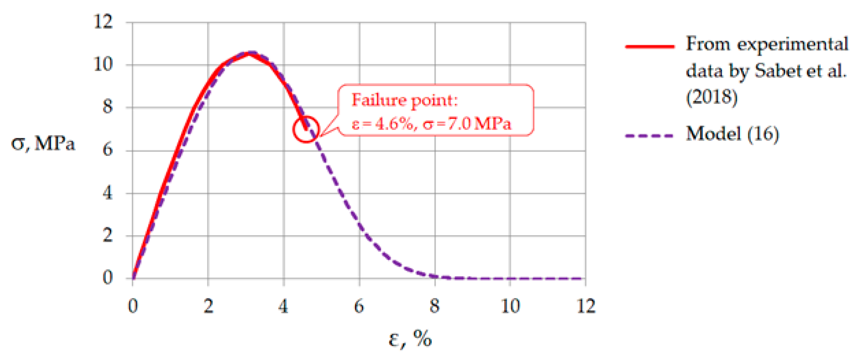
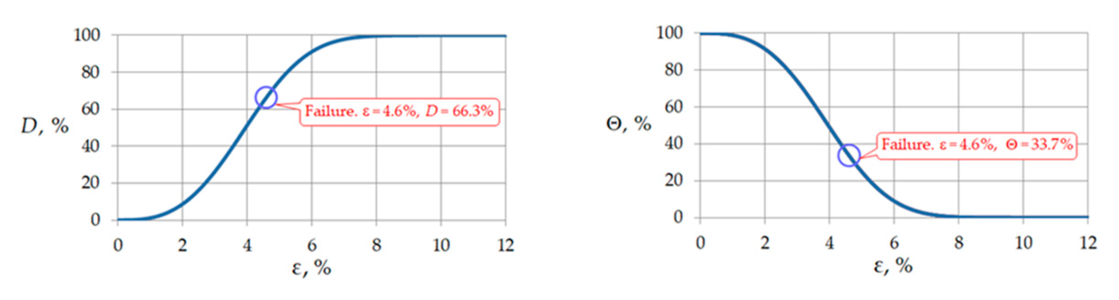
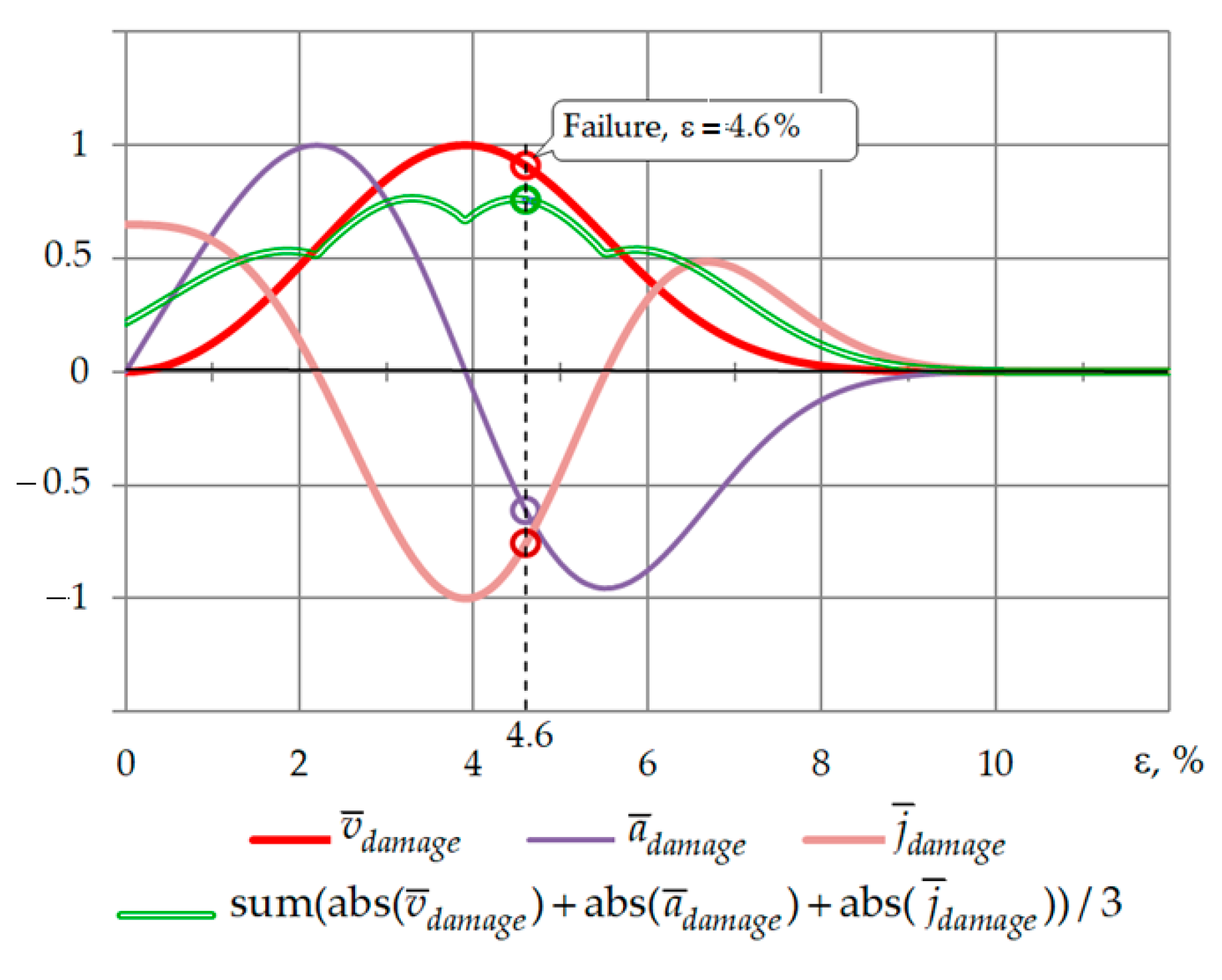
Equation (24) predicts that the damage rate is proportional to the loading rate. The influence of the loading rate on the crack opening rate using an experimental method was investigated in [29], where it was shown that if the load rate increases from 17.1 mm/s to 1750 mm/s (i.e., by about 100 times), then the crack opening rate increases at the same ratio (from 0.02 m/s to 2 m/s). A similar dependence is predicted by Equation (24).

The plots of Equations (24)–(26) for the examples in Figure 2 are shown in Figure 5.

4. Example

Let us consider the application of Equations (10)–(26) to the modeling of a sample of trabecular bone tissue. As the initial data, we used the results of experiments published in [26]. In the experiments in [26], the samples had the shape of a cylinder with a height of 8 mm and a diameter of 4 mm. The samples were loaded until destruction at a rate $v_{load}=0.005 \mathrm{mm}/\mathrm{s}$ that, according to (20), corresponds to $v_{load,\mathsf{\epsilon }}=0.000625 1/s$ (or 0.0625% strain per second). The experimental curve from [26] is shown in Figure 6 (red line). At the extremum point, ${\epsilon }_{extr}^{test}=0.031$ and ${\sigma }_{extr}^{test}=10.56 \mathrm{MPa}$. At the failure point, $\mathsf{\epsilon }=0.046$ and $\sigma =7.00 \mathrm{MPa}$. The same figure shows the plot of Equation (16) (dotted line). Figure 7, Figure 8 and Figure 9 shows function plots $D$ and $,$ $v_{damage}$, $a_{damage}$ and $j_{damage}$.

A comparison of the plots in Figure 6, Figure 7, Figure 8 and Figure 9 leads to the following conclusions.

• The damage rate $(v_{damage})$ increases non-linearly with increasing $\epsilon$ and reaches a peak if $\mathsf{\epsilon }=3.9\%$. The failure point is located near the rate peak, at $\mathsf{\epsilon }=4.6\%$, $v_{damage}=14.939·{10}^{-3}{\mathrm{s}}^{-1}$ and $D=66.3\%$.
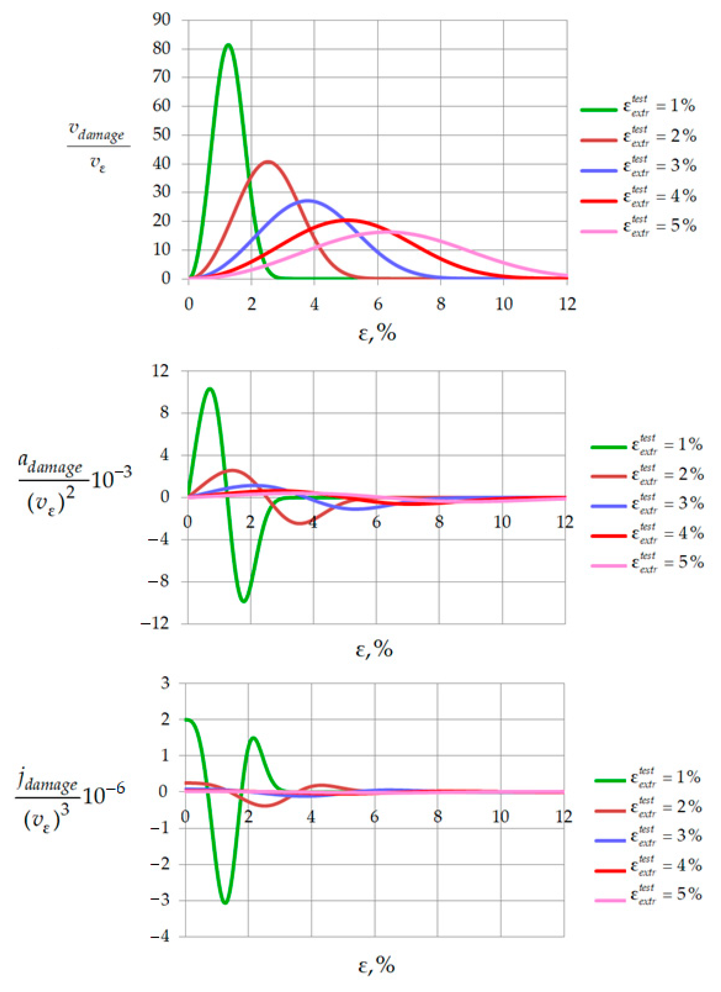
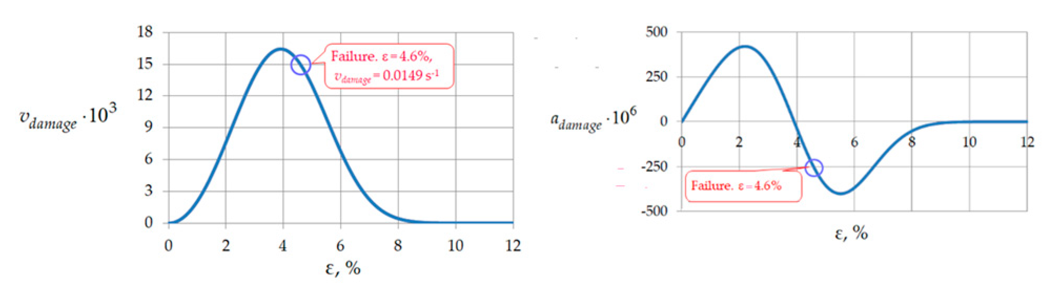
• Figure 6, Figure 7, Figure 8 and Figure 9 show the data corresponding to the download rate $v_{load}=0.005 \mathrm{mm}/\mathrm{s}=5·{10}^{-6}\mathrm{m}/\mathrm{s}$. This is a quasi-static load, in which the absolute value of acceleration ($a_{damage}$) at the failure point is a small value that can be ignored ($a_{damage}=257·{10}^{-6}{\mathrm{s}}^{-1}$). Nevertheless, if the rate of external influence increases, for example, to 5 m/s (18 km/h), that is, by ${10}^6$ times, then, theoretically, the acceleration (25) will increase by ${10}^{12}$ times (then, $a_{damage}=257·{10}^6{\mathrm{s}}^{-1}$), and this will inevitably lead to the bone fracture. The failure point is located near the negative peak of function $a_{damage}=a_{damage}(\epsilon )$ (Figure 8).
• The jerk ($j_{damage}$) shows how fast the acceleration changes. In the considered example, at the failure point, $j_{damage}=19.108·{10}^{-6}{\mathrm{s}}^{-3}$. This is a negligible value. However, if $v_{load}=5\mathrm{m}/\mathrm{s}$, then the jerk (26) will grow ${10}^{18}$ times and will be $j_{damage}=19.108·{10}^{12}{\mathrm{s}}^{-3}$. The failure point is located near the negative peak of function $j_{damage}=j_{damage}(\epsilon )$ (Figure 9).
• It is important to note that the fracture point is close to the peak values of the damage rate, as well as of the acceleration and jerk (Figure 8 and Figure 9). This indicates that the destruction occurred with the greatest combined effect of the damage rate, acceleration and jerk. Thus, a quantitative assessment of the overall impact of the damage rate, as well as of the acceleration and jerk, can be taken into account in predicting the fracture risk.

5. Application of the Damage Function Derivatives in Destruction Prediction

5.1. The Damage Function and Its Derivatives

Even without reference to the example discussed above (Figure 6 and Figure 7), engineering intuition suggests that the rate, acceleration and jerk of the damage process are somehow related to the strength of the quasi-brittle material. How can we obtain quantitative assessment of the influence of velocity and other kinetic characteristics of the destruction process of a quasi-brittle material on its strength under uniaxial compression? To solve this problem, we turned again to the physical sense of the derivatives of the damage function $D$ (12). All components of this function have a clear physical meaning and can be determined as the result of standard uniaxial compression tests. The function $D$ shows the change in the proportion of damaged material depending on the strain. It is important to note that Equation (12) is differentiable. The first derivative ($v_{damage}$) shows how quickly the proportion of the damaged material ($D$) increases depending on time $t$ (21). The second derivative ($a_{damage}$) shows how fast the rate ($v_{damage}$) changes depending on time (22). The third derivative (jerk) shows how fast the second derivative (acceleration) changes with time, etc. Higher derivatives are not often used in engineering practice, so the terms for denoting their physical content still required consensus. Formally, all the derivatives of the damage function $D$ (12) can be represented in the following form:

$$v_{damage}=D^{(1)}=\frac{dD}{dt}=\frac{dD}{d\epsilon }\frac{d\epsilon }{dt}$$

(27)

$$a_{damage}=D^{(2)}=\frac{d{D}^{(1)}}{dt}=\frac{d{D}^{(1)}}{d\epsilon }\frac{d\epsilon }{dt}$$

(28)

$$j_{damage}=D^{(3)}=\frac{d{D}^{(2)}}{dt}=\frac{d{D}^{(2)}}{d\epsilon }\frac{d\epsilon }{dt},\dots$$

(29)

$$D^{(n)}=\frac{d{D}^{(n-1)}}{dt}=\frac{d{D}^{(n-1)}}{d\epsilon }\frac{d\epsilon }{dt}$$

(30)

The practical significance of Equations (27)–(30) lies in the possibility of their use in models for predicting destruction of a quasi-brittle material under uniaxial compression, which is mentioned in Section 5 and discussed in more detail in the next subsection.

5.2. Application of the Damage Function and Its Derivatives to the Prediction of Destruction

Let us consider the possible application of Equations (27)–(30) for predicting the destruction of a quasi-brittle material under uniaxial compression. The analysis of the plots of damage rate, acceleration and jerk in the abovementioned example (Figure 6 and Figure 7) leads to confidence in the reality of such a possibility. From the physical point of view, it is logical to assume that the probability of material destruction is proportional to the combined influence of rate, acceleration and jerk. To take into account the joint influence of rate, acceleration and jerk, we transformed these functions to a dimensionless, normalized to one, form. To do this, we divided both parts of each of Equations (24)–(26), respectively, by $max(\mathrm{abs}(v_{damage}))$, $max(\mathrm{abs}(a_{damage}))$ and $max(\mathrm{abs}(j_{damage}))$. Thus, we obtained functions that we denoted as ${\stackrel{-}{v}}_{damage}$, ${\stackrel{-}{a}}_{damage}$ and ${\stackrel{-}{j}}_{damage}$. Accordingly, the values of these functions were equal to the dimensionless estimates of the influence of rate, acceleration and jerk on material destruction. The plots of the functions are shown in Figure 10.

The total effect of rate, acceleration and jerk on material damage can be determined as the average of three estimates:

$$\Psi =\Psi (\epsilon )=\mathrm{sum}(\mathrm{abs}({\stackrel{-}{v}}_{damage})+\mathrm{abs}({\stackrel{-}{a}}_{damage})+\mathrm{abs}({\stackrel{-}{j}}_{damage}))/3$$

(31)

It is logical to assume that, theoretically, the maximum of Equation (31) corresponds to fracture. The graph of Equation (31) is shown in Figure 10 with a double green line. Two extrema on this line are interesting: at $\epsilon =3.3\%$ and $\epsilon =4.5\%$. The abscissa of one of the extrema ($\epsilon =4.5\%$) almost coincides with the experimental value of the abscissa ($\epsilon =4.6\%$), which corresponds to the fracture point [26].

In Figure 10, it can be seen that failure of the sample corresponds to a change in the sign of acceleration, that is, the compressive strain decrease. Consequently, the frictional force in the contact zone of the particles also decreases, which can lead to shear of the particles, for example, in concrete or rocks. As for the trabecular bone tissue, hypothetically, the change in the sign of acceleration and jerk (Figure 8) may be associated with the appearance of local stretching of the trabecula, which does not contradict the experiments of Turunen et al. [30], who found that, under loading, the structure of cancellous bone tissue demonstrates an alternation of positive and negative local volumetric deformities. Thus, rate, acceleration and jerk (27)–(29) make it possible to obtain an adequate prognosis of destruction of the trabecular bone tissue. Maximum (31), as one of the criteria for failure under uniaxial loading, can be taken into account in further studies.

It should be noted that only the first, second and third derivatives are taken into account in Equation (31). More derivatives can be used to account for more factors. For this, using Equation (30), we rewrote Equation (31) in the general form (32):

$$\Psi =\Psi (\epsilon )=\mathrm{sum}(\mathrm{abs}{D}^{(1)}+\mathrm{abs}{D}^{(2)}+\dots +\mathrm{abs}{D}^{(n)})/n$$

(32)

Equations (27)–(30) can be determined analytically or numerically.

Equation (31) shows the simplest case of using rate, acceleration and jerk to predict fracture, that is, it is assumed that dimensionless estimates of the rate effect, acceleration and jerk equally contribute to material fracture. It would be logical and more realistic to introduce weighting factors. However, the question of justifying the weighting coefficients remains open. Therefore, the author does not offer Equation (31) as a replacement for the generally accepted criteria and estimates of damage, but only shows another possible application of the damage function and its derivatives.

6. Discussion

Methodological Aspects of Modeling Trabecular Bone Tissue

As noted above, trabeculae are periodically renewed, as a result of which the age of various trabeculae and, consequently, their mechanical characteristics do not coincide. For example, according to [31], the strength of the cancellous bone tissue can range from 0.15 to 13.7 MPa. Due to the difference in the age of trabeculae and other factors, the real structure of trabeculae is heterogeneous, and each of its fragments is unique, as discussed in [32]. The heterogeneity of the trabecular bone tissue significantly complicates the modeling, which is necessary, first of all, to assess the risk of bone fractures.

One of the methods of modeling structures as mechanical analogs of trabecular bone tissue is the finite element method (FEM) [32,33]. This is a computer-based method, the practical application and capabilities of which positively correlate with the development of computer technologies. New FEM models, which take into account the inhomogeneity of trabeculae, anisotropy and nonlinear behavior of samples of trabecular bone tissue, allow us to study the functioning of the trabecular bone in more detail [34]. However, the limiting factor in nonlinear FEM models is the relatively high cost of their computer implementation [32,35]. Therefore, in some cases, the use of simplified FEM models continues, in which the inhomogeneity and asymmetry of the elastic characteristics of real bone tissue is ignored since it is assumed that the finite element material is homogeneous, isotropic and linearly elastic [36]. In simplified models, the elastic properties of the material are characterized by two constants (Young’s modulus and Poisson’s ratio). In more complex models, models of anisotropic materials are used, the elastic properties of which are characterized by a large number of constants—from three in the simplest case to 21 in the case of the most general type of anisotropy [37]. Nevertheless, the use of various models and a comparative analysis of the simulation results make it possible to overcome difficulties, the reasons for which are that the experiments contain errors and the models use simplifications, and therefore reasonable questions always arise, which, at the same time, motivate the search for new solutions [32,38,39].

An analysis of the available literature shows that a new and more complex model does not always guarantee a better result compared to a simple but physically adequate model. In this regard, in the context of this article, a recent study [34] is of scientific and practical interest, in which, in particular, it is showed that “heterogeneous anisotropic models accurately predicted the apparent elastic modulus but were no better than a simple homogeneous isotropic model” [34]. In other words, the values of the apparent elastic modulus calculated using two different models are almost the same. Such a coincidence confirms the adequacy of both the complex model and the simple model. Of course, the anisotropic model allows us to get a more detailed idea of the features of the sample behavior during loading. However, in some cases, it is advisable to use a simpler model. In this case, the adequacy of a simple isotropic model can be explained with the following considerations. For example, if both models are adequate, then the experimental load displacement plots for the trabecular tissue sample should coincide with the theoretical plots for both the anisotropic model and the isotropic model.

The experimental load displacement plot contains the primary data on the behavior of the sample during loading. If the experimental load displacement plot coincides with the plot for both the simplified and anisotropic models, it means that the isotropic model directly or indirectly takes into account the same factors as the anisotropic model. Thus, in the study cited above [34], we found confirmation that it is not always necessary to strive for a formal complication of the model. In other words, the methodological guideline in this case may be the principle concerning the choice of theory, known as Ockham’s razor: do not multiply entities beyond the need [40,41]. Essentially, the development of a model of damage to a quasi-brittle material for determining static and kinematic characteristics (10)–(26) during uniaxial compression is based on this principle. Namely, Section 1.3 was fulfilled, and characteristics (10)–(26) were obtained without postulating the damage function and without using the law of softening of a quasi-brittle material on the descending branch of the load displacement plot under uniaxial compression.

Let us pay attention to the manifestations of symmetry and asymmetry of the object of research and the process of its functioning. Uniaxial compression can be considered to be a special case of an axisymmetric problem of mechanics. The trabecular bone tissue fills the proximal part of the human femur. At the same time, the right and left femurs are symmetrical, but the external symmetry hides the asymmetry and uniqueness of the structure of the trabecular tissue [32].

The model proposed above can be used to analyze not only trabecular bone tissue, but also some other quasi-brittle materials. For example, the previous version of the proposed model (similar to the Furamura model [42,43]) was used for the analysis of low- and high-strength concrete (30 and 70 MPa) [44]. However, the details of the answer require separate consideration in another article.

Remark 3.

It should be noted that this article considers the quasi-static uniaxial compression of not too rigid materials, whereas in practice, there is three-dimensional dynamic loading of various materials. Accordingly, the application scope of the obtained results is limited.

7. Conclusions

Based on the results of the study presented above, the following conclusions can be made:

• The model of damage accumulation of a quasi-brittle material under uniaxial compression is substantiated, in which the final Equation (12) corresponds to the Weibull distribution law, which is confirmed by the equivalence of Equations (5) [22] and (12) [8] under condition (13).
• A model of the behavior of a quasi-brittle material under loading is described, in which the elastic modulus of the material does not change under loading at the pre-peak and post-peak loading stages (despite the decrease in the stiffness of the sample with its gradual damage) (Section 2).
• The analytical relations for calculating the rate, acceleration and jerk of the damage process are justified (Section 3.2).
• The possibility of predicting material destruction using the damage function and its derivatives is investigated. It is established that the predicted peak of the combined effect of rate, acceleration and jerk of the damage process is of practical interest as an additional criterion of destruction (Section 5).
• Application limitations to the obtained results are noted (Section 6, Remark 3).

References

- Xing, X.; Cheng, R.; Cui, G.; Liu, J.; Gou, J.; Yang, C.; Li, Z.; Yang, F. Quantification of the temperature threshold of hydrogen embrittlement in X90 pipeline steel. Mater. Sci. Eng. A 2021, 800, 140118. [Google Scholar] [CrossRef]
- Park, Y.; Cheong, E.; Kwak, J.G.; Carpenter, R.; Shim, J.H.; Lee, J. Trabecular bone organoid model for studying the regulation of localized bone remodeling. Sci. Adv. 2021, 7, eabd6495. [Google Scholar] [CrossRef]
- Cowin, S.C. Tissue growth and remodeling. Annu. Rev. Biomed. Eng. 2004, 6, 77–107. [Google Scholar] [CrossRef] [PubMed]
- Oftadeh, R.; Perez-Viloria, M.; Villa-Camacho, J.C.; Vaziri, A.; Nazarian, A. Biomechanics and mechanobiology of trabecular bone: A review. J. Biomech. Eng. 2015, 137, 010802. [Google Scholar] [CrossRef] [PubMed] [Green Version]
- Roesler, H. The history of some fundamental concepts in bone biomechanics. J. Biomech. 1987, 20, 1025–1034. [Google Scholar] [CrossRef]
- Sabet, F.A.; Raeisi Najafi, A.; Hamed, E.; Jasiuk, I. Modelling of bone fracture and strength at different length scales: A review. Interface Focus 2016, 6, 20150055. [Google Scholar] [CrossRef] [Green Version]
- Alcântara, A.C.S.; Assis, I.; Prada, D.; Mehle, K.; Schwan, S.; Costa-Paiva, L.; Skaf, M.S.; Wrobel, L.C.; Sollero, P. Patient-Specific Bone Multiscale Modelling, Fracture Simulation and Risk Analysis—A Survey. Materials 2020, 13, 106. [Google Scholar] [CrossRef] [Green Version]
- Kolesnikov, G.; Meltser, R. A Damage Model to Trabecular Bone and Similar Materials: Residual Resource, Effective Elasticity Modulus, and Effective Stress under Uniaxial Compression. Symmetry 2021, 13, 1051. [Google Scholar] [CrossRef]
- Pugno, N.M. Dynamic quantized fracture mechanics. Int. J. Fract. 2006, 140, 159–168. [Google Scholar] [CrossRef] [Green Version]
- Sihota, P.; Yadav, R.N.; Dhaliwal, R.; Bose, J.C.; Dhiman, V.; Neradi, D.; Karn, S.; Sharma, S.; Aggarwal, S.; Goni, V.G.; et al. Investigation of mechanical, material and compositional determinants of human trabecular bone quality in type 2 diabetes. J. Clin. Endocrinol. Metabol. 2021, 5, e2271–e2289. [Google Scholar] [CrossRef]
- Junqueira, L.C.; Carneiro, J. Basic Histology, Text and Atlas, 10th ed.; Foltin, J., Lebowitz, H., Boyle, P.J., Eds.; Lange Medical Books, McGraw-Hill, Medical Pub. Division: New York, NY, USA, 2003; p. 144. Available online: https://archive.org/details/basichistologyte0000junq/page/144/mode/2up (accessed on 7 September 2021).
- Hambli, R. A quasi-brittle continuum damage finite element model of the human proximal femur based on element deletion. Med Biol. Eng. Comput. 2013, 51, 219–231. [Google Scholar] [CrossRef] [Green Version]
- Hambli, R.; Bettamer, A.; Allaoui, S. Finite element prediction of proximal femur fracture pattern based on orthotropic behaviour law coupled to quasi-brittle damage. Med Eng. Phys. 2012, 34, 202–210. [Google Scholar] [CrossRef] [PubMed]
- Yadav, R.N.; Sihota, P.; Uniyal, P.; Neradi, D.; Bose, J.C.; Dhiman, V.; Neradi, D.; Karn, S.; Sharma, S.; Aggarwal, S.; et al. Prediction of mechanical properties of trabecular bone in patients with type 2 diabetes using damage based finite element method. J. Biomech. 2021, 123, 110495. [Google Scholar] [CrossRef] [PubMed]
- Gao, H. Application of fracture mechanics concepts to hierarchical biomechanics of bone and bone-like materials. Int. J. Fract. 2006, 138, 101–137. [Google Scholar] [CrossRef]
- Nguyen, T.T.; Thai, H.T.; Ngo, T. Optimised mix design and elastic modulus prediction of ultra-high strength concrete. Constr. Build. Mater. 2021, 302, 124150. [Google Scholar] [CrossRef]
- Stepanova, L.V.; Igonin, S.A. Rabotnov damage parameter and description of delayed fracture: Results, current status, application to fracture mechanics, and prospects. J. Appl. Mech. Tech. Phys. 2015, 56, 282–292. [Google Scholar] [CrossRef]
- Liu, D.; He, M.; Cai, M. A damage model for modeling the complete stress–strain relations of brittle rocks under uniaxial compression. Int. J. Damage Mech. 2018, 27, 1000–1019. [Google Scholar] [CrossRef]
- Feng, W.; Qiao, C.; Niu, S.; Jia, Z. An Improved Strain-Softening Damage Model of Rocks Considering Compaction Nonlinearity and Residual Stress under Uniaxial Condition. Geotech. Geol. Eng. 2020, 38, 1217–1235. [Google Scholar] [CrossRef]
- Lemaitre, J.; Dufailly, J. Damage measurements. Eng Fract Mech. 1987, 28, 643–661. [Google Scholar] [CrossRef]
- Qu, P.F.; Zhu, Q.Z. A Novel Fractional Plastic Damage Model for Quasi-brittle Materials. Acta Mech. Solida Sin. 2021, in press. [Google Scholar] [CrossRef]
- Chen, S.; Cao, X.; Yang, Z. Three dimensional statistical damage constitutive model of rock based on Griffith strength criterion. Geotech. Geol. Eng. 2021, in press. [Google Scholar] [CrossRef]
- Zhang, X.X.; Ruiz, G.; Yu, R.C.; Tarifa, M. Fracture behaviour of high-strength concrete at a wide range of loading rates. Int. J. Impact Eng. 2009, 36, 1204–1209. [Google Scholar] [CrossRef] [Green Version]
- Kirane, K.; Bažant, Z.P. Microplane damage model for fatigue of quasibrittle materials: Sub-critical crack growth, lifetime and residual strength. Int. J. Fatigue 2015, 70, 93–105. [Google Scholar] [CrossRef]
- Abdullah, T.; Kirane, K. Continuum damage modeling of dynamic crack velocity, branching, and energy dissipation in brittle materials. Int. J. Fract. 2021, 229, 15–37. [Google Scholar] [CrossRef]
- Sabet, F.; Jin, O.; Koric, S.; Jasiuk, I. Nonlinear micro-CT based FE modeling of trabecular bone—Sensitivity of apparent response to tissue constitutive law and bone volume fraction. Int. J. Numer. Methods Biomed. Eng. 2018, 34, e2941. [Google Scholar] [CrossRef] [PubMed]
- Della Corte, A.; Giorgio, I.; Scerrato, D. A review of recent developments in mathematical modeling of bone remodeling. Proc. Inst. Mech. Eng. Part H J. Eng. Med. 2020, 234, 273–281. [Google Scholar] [CrossRef]
- Eager, D.; Pendrill, A.M.; Reistad, N. Beyond velocity and acceleration: Jerk, snap and higher derivatives. Eur. J. Phys. 2016, 37, 065008. [Google Scholar] [CrossRef]
- Tarifa, M.; Poveda, E.; Yu, R.C.; Zhang, X.; Ruiz, G. Effect of loading rate on high-strength concrete: Numerical simulations. In FraMCoS-8, Proceedings of the 8th International Conference on Fracture Mechanics of Concrete and Concrete Structures, University of Castilla-La Mancha, Toledo, Spain, 10–14 March 2013; van Mier, J.G.M., Ruiz, G., Andrade, C., Yu, R.C., Zhang, X.X., Eds.; Electronic publication: University of Castilla-La Mancha: Toledo, Spain; pp. 953–963. Available online: https://framcos.org/FraMCoS-8/p422.pdf (accessed on 7 September 2021).
- Turunen, M.J.; Le Cann, S.; Tudisco, E.; Lovric, G.; Patera, A.; Hall, S.A.; Isaksson, H. Sub-trabecular strain evolution in human trabecular bone. Sci. Rep. 2020, 10, 13788. [Google Scholar] [CrossRef] [PubMed]
- Schoenfeld, C.M.; Lautenschlager, E.P.; Meyer, P.R. Mechanical properties of human cancellous bone in the femoral head. Med. Biol. Engng. 1974, 12, 313–317. [Google Scholar] [CrossRef] [PubMed]
- Wood, Z.; Lynn, L.; Nguyen, J.T.; Black, M.A.; Patel, M.; Barak, M.M. Are we crying Wolff? 3D printed replicas of trabecular bone structure demonstrate higher stiffness and strength during off-axis loading. Bone 2019, 127, 635–645. [Google Scholar] [CrossRef] [PubMed]
- Sabet, F.A.; Koric, S.; Idkaidek, A.; Jasiuk, I. High-Performance Computing Comparison of Implicit and Explicit Nonlinear Finite Element Simulations of Trabecular Bone. Comput. Methods Programs Biomed. 2021, 200, 105870. [Google Scholar] [CrossRef] [PubMed]
- Yu, Y.E.; Hu, Y.J.; Zhou, B.; Wang, J.; Guo, X.E. Microstructure Determines Apparent-Level Mechanics Despite Tissue-Level Anisotropy and Heterogeneity of Individual Plates and Rods in Normal Human Trabecular Bone. J. Bone Miner. Res. 2021, in press. [Google Scholar] [CrossRef] [PubMed]
- Bevill, G.; Keaveny, T.M. Trabecular bone strength predictions using finite element analysis of micro-scale images at limited spatial resolution. Bone 2009, 44, 579–584. [Google Scholar] [CrossRef] [PubMed]
- Bennison, M.B.; Pilkey, A.K.; Lievers, W.B. Evaluating a theoretical and an empirical model of “side effects” in cancellous bone. Med Eng. Phys. 2021, 8–15. [Google Scholar] [CrossRef]
- Van Rietbergen, B.; Odgaard, A.; Kabel, J.; Huiskes, R. Direct mechanics assessment of elastic symmetries and properties of trabecular bone architecture. J. Biomech. 1996, 29, 1653–1657. [Google Scholar] [CrossRef]
- Unnikrishnan, G.U.; Gallagher, J.A.; Hussein, A.I.; Barest, G.D.; Morgan, E.F. Elastic anisotropy of trabecular bone in the elderly human vertebra. J. Biomech. Eng. 2015, 137, 114503. [Google Scholar] [CrossRef] [PubMed] [Green Version]
- Cowin, S.C.; Mehrabadi, M.M. Identification of the elastic symmetry of bone and other materials. J. Biomech. 1989, 22, 503–515. [Google Scholar] [CrossRef]
- Thunder, S. There is no reason to replace the Razor with the Laser. Synthese 2021, in press. [Google Scholar] [CrossRef]
- Rodriguez-Fernández, J. Ockham’s razor. Endeavour 1999, 23, 121–125. [Google Scholar] [CrossRef]
- Baldwin, R.; North, M.A. Stress-strain curves of concrete at high temperature-A review. Fire Saf. Sci. 1969, 785, 1. Available online: http://www.iafss.org/publications/frn/785/-1/view/frn_785.pdf (accessed on 10 October 2020).
- Stojković, N.; Perić, D.; Stojić, D.; Marković, N. New stress-strain model for concrete at high temperatures. Teh. Vjesn. 2017, 24, 863–868. [Google Scholar]
- Kolesnikov, G. Analysis of Concrete Failure on the Descending Branch of the Load-Displacement Curve. Crystals 2020, 10, 921. [Google Scholar] [CrossRef]
Publisher’s Note: MDPI stays neutral with regard to jurisdictional claims in published maps and institutional affiliations. |
© 2021 by the author. Licensee MDPI, Basel, Switzerland. This article is an open access article distributed under the terms and conditions of the Creative Commons Attribution (CC BY) license (https://creativecommons.org/licenses/by/4.0/).
Share and Cite
Kolesnikov, G. Damage Function of a Quasi-Brittle Material, Damage Rate, Acceleration and Jerk during Uniaxial Compression: Model and Application to Analysis of Trabecular Bone Tissue Destruction. Symmetry 2021, 13, 1759. https://doi.org/10.3390/sym13101759
Kolesnikov G. Damage Function of a Quasi-Brittle Material, Damage Rate, Acceleration and Jerk during Uniaxial Compression: Model and Application to Analysis of Trabecular Bone Tissue Destruction. Symmetry. 2021; 13(10):1759. https://doi.org/10.3390/sym13101759
Chicago/Turabian StyleKolesnikov, Gennady. 2021. "Damage Function of a Quasi-Brittle Material, Damage Rate, Acceleration and Jerk during Uniaxial Compression: Model and Application to Analysis of Trabecular Bone Tissue Destruction" Symmetry 13, no. 10: 1759. https://doi.org/10.3390/sym13101759
APA StyleKolesnikov, G. (2021). Damage Function of a Quasi-Brittle Material, Damage Rate, Acceleration and Jerk during Uniaxial Compression: Model and Application to Analysis of Trabecular Bone Tissue Destruction. Symmetry, 13(10), 1759. https://doi.org/10.3390/sym13101759