Abstract
Best practices in studies of developmental instability, as measured by fluctuating asymmetry, have developed over the past 60 years. Unfortunately, they are haphazardly applied in many of the papers submitted for review. Most often, research designs suffer from lack of randomization, inadequate replication, poor attention to size scaling, lack of attention to measurement error, and unrecognized mixtures of additive and multiplicative errors. Here, I summarize a set of best practices, especially in studies that examine the effects of environmental stress on fluctuating asymmetry.
1. Introduction
Fluctuating asymmetry, the developmental variation that manifests as random bilateral, radial, translatory, helical, or self-similar asymmetry, has had a long, sometimes controversial, history. In the early 1930s, Boris Astaurov [1] and Wilhelm Ludwig [2] recognized fluctuating asymmetry as a special kind of asymmetry. They both published their work in German-language monographs. These first studies were mainly descriptive. Astaurov, for example, described the translatory and bilateral asymmetry of marine polychaetes. Ludwig recognized the population aspects of random developmental variation, recognized deviations from helical symmetry, developed an index of asymmetry like those that would appear 20 years later, and coined the term fluctuating asymmetry. In 1953, Kenneth Mather [3] published the first English-language paper that was to attract widespread interest, Genetical control of stability in development. He studied bristle asymmetry and genic balance in Drosophila melanogaster. For an index of average asymmetry, he used the variance of the difference between bristle counts on left and right sides. Estimates of dispersion like this are still the preferred indices of fluctuating asymmetry. He used the asymmetry variance as an estimate of developmental instability, comparing that of two inbred stocks and their F1 and F2 hybrids. He also selected for increased and decreased asymmetry, to see if developmental stability was heritable. It was not until 1962, however, that Leigh Van Valen [4] resurrected the term fluctuating asymmetry to describe what Astaurov, Ludwig, Mather, and others had been studying in the previous 30 years. Since the early 1960s, the number of papers mentioning fluctuating asymmetry has grown tremendously (Figure 1) and shows no signs of abating.
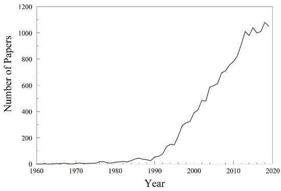
Figure 1.
Number of papers per year mentioning fluctuating asymmetry, over the past 60 years. Data from Google Scholar; count for 2020 is estimated from the count on 11 November 2020.
Best practices for studies of fluctuating asymmetry were worked out decades ago, beginning with Palmer and Strobeck’s [5] classic paper, Fluctuating asymmetry: measurement, analysis, patterns, and several follow-up papers by these and other authors. Yet many of the papers I review for Symmetry and other journals seem to be unfamiliar with the earlier literature, and are only vaguely familiar with the best practices delineated by Palmer and Strobeck and then refined over the last 35 years. Many recent papers, for example, are inadequately replicated, confound potential stressors, exhibit poor attention to size scaling, do not take measurement error into account, and ignore mixtures of additive and multiplicative errors. Many of these studies are deeply flawed. In this review, I provide an up-to-date summary of the best practices as I understand them. I rely heavily on Palmer and Strobeck [5], subsequent refinements to their recommendations [6,7], and several of my own papers. Some of my recommendations reflect my own judgement and may not be shared by others.
2. Fluctuating Asymmetry and Developmental Instability
The first recognition of developmental instability that I am aware of is in a paper on monozygotic twins, published in 1919 by C.H. Danforth [8]. Monozygotic twins share a common intrauterine environment and a common genotype, so any differences can be attributed to random developmental variation. In 1920, Sewall Wright [9] also recognized that “irregularity of development” might contribute to phenotypic variation of piebald patches in highly inbred guinea pigs. Furthermore, in 1921, Sumner and Huestis [10] carried the concept of random phenotypic variation one step further, to explain minor asymmetries that were not strictly heritable.
Fluctuating asymmetry, when it was employed by Mather [3], was understood to be an inverse index of developmental stability (or a direct index of its converse, developmental instability). Mather assumed that developmental stability might be closely related to the average fitness (or wellbeing) of individuals in a population.
Beginning in the 1960s, fluctuating asymmetry came to be used to evaluate environmental stress. Valentine, Soulé, and Samallow [11,12], for example, found that fluctuating asymmetry of marine fishes was greater in highly polluted coastal waters of Southern California than in relatively pristine waters to the north and south of major population centers. In the ensuing decades, there have been hundreds, perhaps thousands, of papers influenced, either directly or indirectly, by these two papers.
3. Fluctuating Asymmetry Is a Population Parameter
Fluctuating asymmetry is a population parameter. Because the indices in common use are measures of dispersion, a sample of a population is required. For example, one cannot estimate an asymmetry variance, var(l − r), in a sample of one, where l is a trait value on the left side and r is a trait value on the right side. One can certainly estimate individual asymmetry, d = l − r, but in most cases, there are no degrees of freedom to compare one individual’s developmental instability with another’s. An exception to this rule is with modular organisms, such as plants, which have numerous leaves, flowers, and fruit [13].
Michael Soulé [14] recognized that fluctuating asymmetry is a population parameter. His attempts to find an organism-wide asymmetry parameter failed. Individual asymmetry of one trait is generally uncorrelated with individual asymmetry of other traits on the same individual. The only exception is when traits are part of a single developmental unit [15].
Individual asymmetry is, nevertheless, invoked in studies of sexual selection [16]. Females, for example, may prefer males having more symmetrical sexual ornaments. But one cannot say with certainty that a male having a more symmetrical ornament is more developmentally stable than another male having a less symmetrical ornament. One can only make inferences about populations. One population may have more symmetrical individuals, on average, than another. Furthermore, one may make inferences about subsamples from the same population (males attractive to females versus those unattractive to females, or genotype AA versus genotype aa). To repeat, one cannot declare that any individual has greater developmental stability just because one or more traits are nearly symmetrical.
Fluctuating asymmetry, then, is an index of developmental instability, and is often thought of as being sensitive to stress, either environmental or genetic. Environmental stress includes climate, parasites, pollutants, competition, predation, herbivory, and virtually anything that dissipates energy away from growth and reproduction [17]. I am mainly interested in the effects of pollution or climate change in this brief review, but the principles apply elsewhere.
4. Study Design
One should begin any study with one or more testable (i.e., falsifiable) hypotheses. The hypothesis that polychlorinated biphenyls (PCBs) are stressful agents for aquatic invertebrates might be such a hypothesis. General hypotheses, though, are rarely testable directly, but they can lead to testable predictions. This is the hypothetico-deductive approach. For example, if it is true that PCBs are stressful for aquatic invertebrates, then dragonflies (as a typical insect that has an aquatic stage) emerging from PCB-polluted waters (or exposed to PCBs in the lab) should display greater fluctuating asymmetry than those not exposed to PCBs. This testable prediction assumes that fluctuating asymmetry is, indeed, a valid indicator of stress. That assumption may or may not be true. Consequently, it is always wise, if possible, to examine other indicators of stress, such as growth rate, frequency of phenodeviants, or stress hormones (e.g., cortisol in vertebrates).
Fluctuating asymmetry has been described as a small signal in a sea of noise. Consequently, sample sizes should be large. I prefer more than n = 40 individuals per population or subpopulation, and n = 100 is even better. Moreover, as I point out below, random replicate measurements are essential. Three replicates for continuously varying traits is not too many.
In studies of environmental stress, it is crucial that sample sites (populations) be replicated. Otherwise, it is impossible to generalize to all populations. Finding a difference between organisms at a single treatment site and a single control site proves only that those two populations differ. Both treatment and control sites should be replicated equally. The number of replicate sites will depend upon the variation among sites.
I suggest a small preliminary sample of several control sites to decide whether to put more effort into sampling sites or sampling individuals within sites. This can be accomplished with a variance components analysis of a nested, completely randomized experimental design. For example, imagine that d = |l − r| of some bilateral trait is the dependent variable, and the sources of variation (effects) are populations, individuals within populations, and replicate measurements within individuals within populations. There are thus three variance components to estimate. The largest variance components indicate where the most uncertainty lies. Uncertainty demands a greater sampling effort. The R Project for Statistical Computing has a package (VCA, together with lme4) that will do variance components. Both SPSS and SAS also feature procedures that do variance components.
Studies of fluctuating asymmetry are easily marred by confirmation bias [18], thus it is important that the scoring be randomized and blind. I have done this in the past by coding samples and only revealing a sample’s identity after scoring is completed. If more than one individual is doing the scoring, samples to be scored should be assigned at random.
Finally, whenever possible, one should minimize the interaction between genotype and environment by removing genetic variation. This can be accomplished in an experimental setting with isogametic female lines, vegetatively reproducing organisms, or clonal organisms [19].
5. Choice of Traits
Choice of traits boils down to three classes: continuously varying linear measurements, meristic counts, and shape asymmetry. Researchers can address one or more of these approaches in the same study [20]. Examples of continuous variables include traits such as ear width, bone length and width, and the distance between two landmarks on a fruit fly’s wing. Meristic traits include bristle counts in fruit flies, scale counts in fish, and ridge counts on dermatoglyphic patterns. Shape asymmetry involves geometric morphometrics based upon landmarks in two or three dimensions [21], as well as continuous symmetry measures [17].
Most studies of fluctuating asymmetry concern deviations from bilateral symmetry. However, there are as many other approaches as there are classes of symmetry [17]. Papers in the literature have addressed rotational (radial) symmetry, dihedral symmetry, translatory symmetry, and fractal symmetry. I will not discuss those in detail here, but manifold approaches can be easily generalized from bilateral, mirror symmetry.
6. Choice of an Index
The initial asymmetry indices in the literature were based upon the variance of the difference d between left and right sides, var(d), where d = l − r or d = r − l. The correlation ρ between left and right sides, has also been used, mostly in the older literature.
The correlation coefficient ρ measures the association between left and right sides. Large values of ρ indicate greater symmetry. The more useful inverse measure of symmetry is 1 − ρ; large values of 1 − ρ indicate greater asymmetry.
One advantage of correlation-based asymmetry measures is that they are unitless. However, correlation coefficients have one glaring problem; they are strongly influenced by the range of values, as well as sample size. Both Bradley [22] and Angus [23] remarked on this problem and Palmer and Strobeck [5] reported that asymmetry indices based on correlations lack statistical power and behave differently than other indices. They are not recommended.
The indices based upon measures of dispersion, such as var(d), have their own problems, largely the inefficiency of statistical tests, such as Bartlett’s test, that compare two variances [5]. An alternative measure of dispersion is the mean absolute deviation, or MAD, which is the expectation of the absolute difference between d and the population mean [17]. Since the population mean of d in studies of fluctuating asymmetry is 0, the mean absolute deviation is E|d − μd| = E|d − 0| = E|d|. This index is amenable to analysis of variance, a more robust means of comparing dispersion of two or more populations. In the fluctuating asymmetry literature, this index is often referred to as Levene’s Test. This is now the most widely used index to compare two or more populations.
7. Size Scaling
Size scaling arises because of the way that most organisms, or parts of organisms, grow. Active tissue growth involves the addition of new tissue to old tissue. This results in multiplicative statistical error [24]. To be clear, this is natural variation, not measurement error. If individuals grow in this way, trait values will be lognormally distributed and variances will increase with size. The scaling of the trait variances follows Taylor’s Power Law, var(y) = aμb, where y is a trait value, u is the mean trait value, a is a positive constant characteristic of a particular population, and b is an exponent that usually equals 2 under active tissue growth and multiplicative error [25,26]. The standard way of dealing with this positive size scaling has been to divide d or |d| by either the population mean of l + r, or just l + r. A more logical approach, though, is to use d′ = log l − log r, or equivalently log(l/r), which follows directly from the principle of allometric, active tissue growth [24]. An alternative approach suggested by Pertoldi et al. [25] uses Taylor’s Power Law, originally used to model population densities in ecology [26], to take size scaling into account without the usual transformations.
Use of d′ = log l − log r will usually work if measurement error is very small, or if the range of sizes is small. If measurement error is large, however, one risks generating negative size scaling, an artefact of mixing additive and multiplicative errors and then correcting for the multiplicative errors. Smaller individuals will seem to have greater average asymmetry, and hence will seem to have greater developmental instability. This happens because of the mixture of additive and multiplicative errors. Measurement error is additive, but growth variation is multiplicative.
The solution to this problem is simple but requires replicate samples. By averaging replicates of the same trait, and using the averages in the analysis, one reduces the additive measurement error by half with each round of replication [24]. When confronted with data sets (after the fact) that lacked replication, I have used Box-Cox power transformations to come up with a power parameter λ in between no transform (λ = 1) and a log transform (λ = 0) [17,27]. Pertoldi et al.’s [25] approach to dealing with a value of the power-law exponent, b ≠ 2, will accomplish much the same goal, but without the explicit transformation.
One should always check each population and subpopulation for positive or negative size scaling in any study of fluctuating asymmetry [5]. This can be done by regressing |d| on l + r and examining the scatter of values in an x,y scatterplot. If the spread of |d| increases with size, positive size scaling is indicated. If it decreases with size, negative size scaling is indicated.
However, what if developmental instability really does change with size? One can usually eliminate mixtures of multiplicative and additive error, and one can correct for multiplicative error. If the changes survive these tests, it is safe to say the trends are real.
Measurement error should be estimated in all studies of fluctuating asymmetry. How much of the total variation, var(l + r), is due to measurement error? How much of the asymmetry variation, var(l − r), is due to measurement error? If measurement error is large, there will almost surely be a mixture of additive and multiplicative error for most traits.
8. Composite Indices
Several authors have suggested composite indices of fluctuating asymmetry. Leung et al. [28] recommend two composite indices, CFA 2 and CFA 3. Composite indices provide more powerful statistical tests.
For CFA 2, Leung et al. standardize of a particular trait in a particular individual by the average for that trait among all individuals. For an individual, then, CFA 2 is the sum of the standardized asymmetry across traits. CFA 2 for a single individual j is , where |di| is the absolute value of d = l − r for individual j and trait i, and the number of traits is i = 1 to n.
CFA 3 uses ranks of |d| for each trait, across all individuals in all subpopulations. CFA 3 is then the sum of the ranks. For example, suppose there are n = 25 individuals from a control site and n = 25 from a treatment site. Suppose four traits are examined and individual j is ranked 3rd, 8th, 17th, and 45th on the four traits. Then CFA 3 = 3 + 8 + 17 + 45 = 73 for individual j.
According to Leung et al. [28], CFA 2 is the more powerful index when the di are normally distributed or slightly leptokurtic, while CFA 3 is the more powerful index when di are strongly leptokurtic. Leptokurtosis is common in studies of fluctuating asymmetry and arises naturally in traits that exhibit active tissue growth; the difference between two lognormal distributions is leptokurtic [24].
9. Meta-Analysis of Multiple Species
Vladimir Zakharov [29] suggested that studies of environmental stress are most effective if they incorporate several related species. He called this approach Biotest. Several species are often studied at once when environmental stress is of interest. Valentine et al. [12], mentioned previously, studied three species of marine fish. Raz et al. [27], in another example, studied 12 species of angiosperms on north- and south-facing slopes of Evolution Canyon in Israel. They used Hedges’ g, an index of effect size between two means (standardized mean difference), to place all 12 species on an even footing.
where .
A value of g was estimated for each of the 12 species on the two slopes. Because some of the 12 species were adapted to the north-facing slope while others were adapted to the south-facing slope, there were no differences between the two slopes over all 12 species. There was, however, a significant correlation of r = −0.517 between Hedges’ g and a normalized difference abundance index. Those species having more asymmetrical leaves on the south-facing slope were more abundant on the north-facing slope, and vice versa.
Effect sizes are an extension of the techniques of meta-analysis. Most meta-analyses combine results from completely different experiments or studies of natural variation. The approach that I am recommending is justifiable because different species are semi-independent tests of the same hypothesis regarding an entire community of species.
In any case, even if meta-analytic techniques are not used, effect sizes should always be reported along with parameter estimates (means, standard deviations, and confidence intervals). The community of professional statisticians has railed against the primacy of hypothesis testing and p-values. One can almost always reject the null hypothesis with a large enough sample. Furthermore, p-values are not reflective of effect size; a p < 0.00001 does not indicate a greater effect size than p < 0.05. Effect sizes like Hedges’ g can rectify the weaknesses of p-values. Last year, American Statistician, a publication of the American Statistical Association, published a special issue devoted to Statistical Inference in the 21st Century: A World Beyond p < 0.05 [30]. All publishing scientists should examine it.
10. Checklist for Studies of Environmental Stress
- Decide on a question and how you want to address it. Hypotheses need to be falsifiable.
- Work out an experimental (or observational) design, preferably a blind, randomized one. Study sites (controls and treatments) should be replicated if you want to make general inferences. Lack of replication is inexcusable.
- Choose the species you want to study. A study that examines several species that are either taxonomically or functionally related is better than a study that focuses on one species. The results of a study of a single species cannot be generalized to the entire community.
- Select several traits that are symmetric on average (i.e., the mean of d = 0). Weed out traits that exhibit directional asymmetry or antisymmetry. Any traits that are chosen should be reliably measured, counted, or amenable to geometric morphometrics. A mixture of continuous, meristic, and shape variables is best.
- If possible, conduct a small preliminary study to evaluate variability among sites (populations), among species, among traits, and among replicate measurements. This completely randomized and nested design is amenable to a variance components ANOVA. Use the variance components to decide on final sample sizes. The goal here is to increase the power of any tests necessary to reject the null hypothesis.
- Examine the traits for size scaling, either positive or negative. Make an evaluation with respect to the prevailing error models for each trait, either additive or multiplicative. Active tissue growth generates multiplicative errors, while inert tissue growth generates additive errors. Be aware of any mixing of additive and multiplicative errors.
- Choose the largest sample sizes you can afford. Plan on two or more replicates of each measurement, especially if measurement error is high. Measurement error inflates estimates of fluctuating asymmetry. For meristic traits, replicate counts should match. If they do not, do a third count. In principle, measurement error should be nil for meristic traits.
- Decide on individual asymmetry indices for each trait. Based on the work of Palmer and Strobeck, use either var(l − r) or E|l − r| for additive error models and var(log l − log r) or E|log l − log r| for multiplicative error models. For shape asymmetry, use a Procrustes index for objects that are consistently symmetrical, that is, objects with identifiable and homologous landmarks. For partial or inconsistent objects, lacking such landmarks, a continuous symmetry index can be used.
- Use a composite index of fluctuating asymmetry by combining all traits on an individual into a single index. Be careful not to include traits that have undue effects on the composite index, even after standardization.
- If using E|l − r| or E|log l − log r|, estimate means, variances, standard errors, and 95% confidence intervals for the means for each treatment group and control. Conduct an analysis of variance and estimate effect sizes.
- Use the methods of meta-analysis to combine the several species to test the grand hypothesis regarding an entire community of species.
11. Conclusions
Fluctuating asymmetry is a valuable tool for understanding the developmental repercussions of stress in ecological communities. Much of the stress that we are interested in is of human origin: polychlorinated biphenyls, heavy metals, thermal discharge, crowding of animals under agricultural confinement, and climate change. Good design and implementation of studies should be worked out always before the first sample is taken, and fluctuating asymmetry is no exception.
Funding
This research received no external funding.
Acknowledgments
I acknowledge 30 years of generous support from Berry College. I would like to thank J. Richard Trout and Horace P. Andrews of the Rutgers University Department of Statistics for giving me a thorough grounding in statistics and experimental design. In addition, two anonymous reviewers made several worthwhile suggestions on the manuscript.
Conflicts of Interest
The author declares no conflict of interest.
References
- Astaurov, B.L. Analyse der erblichen Störungsfälle der bilateralen Symmetrie. Z. Indukt. Abstamm. Ver. 1930, 55, 183–262. [Google Scholar] [CrossRef]
- Ludwig, W. Das Rechts-Links Problem im Tierreich und Beim Menschen; Springer: Berlin, Germany, 1932; pp. 1–442. [Google Scholar]
- Mather, K. Genetical control of stability in development. Heredity 1953, 7, 297–336. [Google Scholar] [CrossRef]
- Van Valen, L. A study of fluctuating asymmetry. Evolution 1962, 16, 125–142. [Google Scholar] [CrossRef]
- Palmer, A.R.; Strobeck, C. Fluctuating asymmetry: Measurement, analysis, patterns. Annu. Rev. Ecol. Syst. 1986, 17, 391–421. [Google Scholar] [CrossRef]
- Palmer, A.R. Fluctuating asymmetry analyses: A primer. In Developmental Instability: Its Origins and Evolutionary Implications; Markow, T.A., Ed.; Kluwer: Dordrecht, The Netherlands, 1994; pp. 335–364. [Google Scholar]
- Palmer, A.R.; Strobeck, C. Fluctuating asymmetry analyses revisited. In Developmental Instability: Causes and Consequences; Polak, M., Ed.; Oxford University Press: New York, NY, USA, 2003; pp. 279–319. [Google Scholar]
- Danforth, C.H. Resemblance and difference in twins. J. Hered. 1919, 10, 399–409. [Google Scholar] [CrossRef]
- Wright, S. The relative importance of heredity and environment in determining the piebald pattern of Guinea-Pigs. Proc. Natl. Acad. Sci. USA 1920, 6, 320–332. [Google Scholar] [CrossRef]
- Sumner, F.B.; Huestis, R.R. Bilateral asymmetry and its relation to certain problems of genetics. Genetics 1921, 6, 445–485. [Google Scholar]
- Valentine, D.W.; Soulé, M.E. Effects of p.p’-DDT on developmental fin rays of the grunion, Leuresthes tenuis. US Nat. Mar. Fish. Serv. Fish. Bull. 1973, 71, 921–926. [Google Scholar]
- Valentine, D.W.; Soulé, M.E.; Samallow, P. Asymmetry analysis in fishes: A possible statistical indicator of environmental stress. US Nat. Mar. Fish. Serv. Fish. Bull. 1973, 71, 357–370. [Google Scholar]
- Cowart, N.M.; Graham, J.H. Within- and among-individual variation in fluctuating asymmetry of leaves in the Fig (Ficus carica L.). Int. J. Plant Sci. 1999, 160, 116–121. [Google Scholar] [CrossRef]
- Soule, M. Phenetics of natural populations. II. Asymmetry and evolution in a lizard. Am. Nat. 1967, 101, 141–160. [Google Scholar] [CrossRef]
- Klingenberg, C.P. Morphological integration and developmental modularity. Annu. Rev. Ecol. Evol. Syst. 2008, 39, 115–132. [Google Scholar] [CrossRef]
- Gangestad, S.W.; Thornhill, R.; Yeo, R.A. Facial attractiveness, developmental stability, and fluctuating asymmetry. Evol. Hum. Behav. 1994, 15, 73–85. [Google Scholar] [CrossRef]
- Graham, J.H.; Raz, S.; Hel-Or, H.; Nevo, E. Fluctuating asymmetry: Methods, theory, and applications. Symmetry 2010, 2, 466–540. [Google Scholar] [CrossRef]
- Kozlov, M.G.; Zvereva, E.L.; Kozlov, M.V. Confirmation bias in studies of fluctuating asymmetry. Ecol. Indic. 2015, 57, 293–297. [Google Scholar] [CrossRef]
- Kristensen, T.N.; Pertoldi, C.; Pedersen, L.D.; Andersen, D.H.; Bach, L.; Loeschcke, V. The increase of fluctuating asymmetry in a monoclonal strain of collembolans after chemical exposure—Discussing a new method for estimating the environmental variance. Ecol. Indic. 2004, 4, 73–81. [Google Scholar] [CrossRef]
- Benítez, H.A.; Lemic, D.; Villalobos-Leiva, A.; Bažok, R.; Órdenes-Claveria, R.; Pajač Živković, I.; Mikac, K.M. Breaking symmetry: Fluctuating asymmetry and geometric morphometrics as tools for evaluating developmental instability under diverse agroecosystems. Symmetry 2020, 12, 1789. [Google Scholar] [CrossRef]
- Klingenberg, C.P.; McIntyre, G.S. Geometric morphometrics of developmental instability: Analyzing patterns of fluctuating asymmetry with Procrustes methods. Evolution 1998, 52, 1363–1375. [Google Scholar] [CrossRef]
- Bradley, B.P. Developmental Stability of Drosophila melanogaster under artificial and natural selection in constant and fluctuating environments. Genetics 1980, 95, 1033–1042. [Google Scholar]
- Angus, R.A. Quantifying fluctuating asymmetry—Not all methods are equivalent. Growth 1982, 46, 337–342. [Google Scholar]
- Graham, J.H.; Shimizu, K.; Emlen, J.M.; Freeman, D.C.; Merkel, J. Growth models and the expected distribution of fluctuating asymmetry. Biol. J. Linn. Soc. 2003, 80, 57–65. [Google Scholar] [CrossRef]
- Pertoldi, C.; Kristensen, T.N. A New fluctuating asymmetry index, or the solution for the scaling effect? Symmetry 2015, 7, 327–335. [Google Scholar] [CrossRef]
- Taylor, L.R. Aggregation, variance and the mean. Nat. Cell Biol. 1961, 189, 732–735. [Google Scholar] [CrossRef]
- Raz, S.; Graham, J.H.; Hel-Or, H.; Pavlíček, T.; Nevo, E. Developmental instability of vascular plants in contrasting microclimates at ‘Evolution Canyon’. Biol. J. Linn. Soc. 2011, 102, 786–797. [Google Scholar] [CrossRef]
- Leung, B.; Forbes, M.R.; Houle, D. Fluctuating asymmetry as a bioindicator of stress: Comparing efficacy of analyses involving multiple traits. Am. Nat. 2000, 155, 101–115. [Google Scholar] [CrossRef] [PubMed]
- Zakharov, V.M.; Clarke, G.M. Biotest: A New Integrated Biological Approach for Assessing the Condition of Natural Environments; International Biotest Foundation: Moscow, Russia, 1993; pp. 1–59. [Google Scholar]
- Wasserstein, R.L.; Schirm, A.L.; Lazar, N.A. (Eds.) Statistical Inference in the 21st Century: A World Beyond p < 0.05; Taylor & Francis Online: Abingdon, UK, 2019; Volume 73, pp. 1–401. [Google Scholar]

Publisher’s Note: MDPI stays neutral with regard to jurisdictional claims in published maps and institutional affiliations. |
© 2020 by the author. Licensee MDPI, Basel, Switzerland. This article is an open access article distributed under the terms and conditions of the Creative Commons Attribution (CC BY) license (http://creativecommons.org/licenses/by/4.0/).