Connecting (Anti)Symmetric Trigonometric Transforms to Dual-Root Lattice Fourier–Weyl Transforms

Abstract

Explicit links of the multivariate discrete (anti)symmetric cosine and sine transforms with the generalized dual-root lattice Fourier–Weyl transforms are constructed. Exact identities between the (anti)symmetric trigonometric functions and Weyl orbit functions of the crystallographic root systems $A_1$ and $C_n$ are utilized to connect the kernels of the discrete transforms. The point and label sets of the 32 discrete (anti)symmetric trigonometric transforms are expressed as fragments of the rescaled dual root and weight lattices inside the closures of Weyl alcoves. A case-by-case analysis of the inherent extended Coxeter–Dynkin diagrams specifically relates the weight and normalization functions of the discrete transforms. The resulting unique coupling of the transforms is achieved by detailing a common form of the associated unitary transform matrices. The direct evaluation of the corresponding unitary transform matrices is exemplified for several cases of the bivariate transforms.

1. Introduction

The purpose of this article is to develop an explicit link between the multivariate discrete (anti)symmetric trigonometric transforms [1,2] and generalized dual-root lattice Fourier–Weyl transforms [3,4]. The established correspondence [5] between the (anti)symmetric trigonometric functions and Weyl orbit functions induced by the crystallographic root systems $A_1$ and $C_n$ [6,7] is utilized to interlace the kernels, point and label sets of the discrete transforms. The exact connections among the types of the discrete transforms allow for comparison and migration of the associated multivariate Fourier and Chebyshev methods [8,9,10].

The symmetric and antisymmetric discrete trigonometric transforms [1,2] are introduced as generalizations of the classical sixteen types of univariate discrete cosine (DCT I–VIII) and sine transforms (DST I–VIII) [11]. There exist eight symmetric multivariate discrete cosine transforms (SMDCTs) of types I–VIII and eight antisymmetric multivariate discrete cosine transforms (AMDCTs) of types I–VIII [9]. In addition to the generalized discrete cosine transforms, eight symmetric multivariate discrete sine transforms (SMDSTs) of types I–VIII and eight antisymmetric multivariate discrete sine transforms (AMDSTs) of types I–VIII emerge from the eight standard discrete sine transforms [1,10,12]. Moreover, the antisymmetric trigonometric transforms constitute special cases of the Fourier transforms evolved from the generalized Schur polynomials [13]. The kernels of the entire collection of the multivariate discrete trigonometric transforms are formed by the multivariate (anti)symmetric cosine and sine functions [1]. The symmetry properties of the (anti)symmetric trigonometric functions restrict both points and labels of the corresponding discrete transforms to specifically constructed fundamental domains. The unique positioning of the transform nodes and labels relative to their respective fundamental domains reflects the symmetries and boundary behavior of each type of the (anti)symmetric trigonometric function [9,10]. Resolving the exact isomorphisms between the symmetry groups of the (anti)symmetric trigonometric functions and the affine Weyl groups related to the series of the crystallographic root systems $A_1$ and $C_n$ (${\mathcal{C}}_n$ series) leads to the explicit direct link between the (anti)symmetric trigonometric functions and Weyl orbit functions [5].

The Weyl orbit functions systematize multivariate complex-valued generalizations of the classical trigonometric functions [6,7,8]. The symmetry properties, fundamental domains, and boundary behaviors of the Weyl orbit functions are determined by the innate sign homomorphisms of the Weyl groups. The identity and determinant sign homomorphisms occur for the Weyl groups of all crystallographic root systems, the short and long sign homomorphisms stem from the crystallographic root systems with two root lengths [8]. Formulated on the Weyl group invariant lattices, the discrete Fourier–Weyl transforms constitute multivariate generalizations of the classical discrete trigonometric transforms that utilize as their kernels the Weyl orbit functions. The standard lattice form of the Fourier–Weyl transforms, realized on the refined dual weight [14,15], weight [16,17], and dual root lattices [3], admits further extensions via admissible shifts of the (dual) root and weight lattices [4,18]. It appears that only after taking into account recent Fourier–Weyl transforms with the rescaled shifted dual root lattices point sets and the shifted weight lattices label sets [3,4], the entire family of 32 multivariate discrete (anti)symmetric trigonometric transforms permits embedding into the Fourier–Weyl formalism of the crystallographic root systems ${\mathcal{C}}_n$. Since both (anti)symmetric trigonometric and Fourier–Weyl transforms attain uniform characterization by their complementary unitary transform matrices [4,10], coupling together the ordered label and point sets as well as the weight and normalization functions produces the exact one-to-one correspondence between the unitary matrices of the induced discrete transforms.

Intrinsic in the established one-to-one correspondence, the exact evaluation techniques for the ${\mathcal{C}}_n$ transforms devise a foundation for similar explicit expositions of the Fourier–Weyl transforms related to the remaining infinite series of the crystallographic root systems [4,10]. Furthermore, the actualized coincidence between the (anti)symmetric trigonometric and Fourier–Weyl transforms offers tools for connection and transfer of the discrete Fourier methods [11,19]. The successful interpolation tests for the 2D and 3D (anti)symmetric trigonometric functions [2,9,10,12] indicate matching interpolation behavior of the corresponding Fourier–Weyl transforms as well as relevance of both types of transforms in data processing methods [20]. In particular, the vast pool of recursive algorithms for fast computation of the (multivariate) trigonometric transforms [11] becomes linked to the central splitting of the discrete Fourier–Weyl transforms [21,22] and vice versa. Moreover, the cubature rules [23] of the multivariate Chebyshev polynomials, that are obtained from the (anti)symmetric trigonometric functions [9,10] and associated with the Jacobi polynomials [5,24,25], are further intertwined with the Lie theoretical approach [8,26,27]. The role of the 2D and 3D Fourier–Weyl transforms as tools for solutions of the lattice vibration and electron propagation models [28,29] implies comparable function and direct applicability of the (anti)symmetric trigonometric transforms in solid state physics [30,31] and quantum field theory [32]. The potential diverse applications of both types of discrete transforms also involve image compression [33], laser optics [34], fluid flows [35], magnetostatic modeling [36], and micromagnetic simulations [37].

The paper is organized as follows. In Section 2, a unified description of the dual-root lattice Fourier–Weyl transforms related to the crystallographic root systems ${\mathcal{C}}_n$ is contained. Section 3 comprises 32 types of point and label sets together with the corresponding normalization and weight functions inherent in the (anti)symmetric trigonometric transforms. Section 4 explicitly develops the link between the point and label sets of the discrete transforms. In Section 5, the Fourier–Weyl normalization and weight functions are converted to their trigonometric counterparts. Section 6 connects the unitary matrices induced by the Fourier–Weyl transforms and (anti)symmetric trigonometric transforms as well as exemplifies specific cases of types $\mathrm{II}$ and $\mathrm{VII}$. Comments and follow-up questions are included in the last section.

2. Dual-Root Lattice Fourier–Weyl Transforms

2.1. Root and Weight Lattices

This section recalls pertinent properties of the irreducible crystallographic root systems $A_1$ and $C_n$, $n\ge 2$ that are necessary for the description of the associated lattices and Weyl orbit functions [38,39]. In order to facilitate the mathematical exposition of this paper, the symbol of the unified series ${\mathcal{C}}_n$, $n\in \mathbb{N}$ is introduced by

$${\mathcal{C}}_n=\left\{\begin{array}{cc}{A}_1\hfill & n=1,\hfill \\ C_n\hfill & n\ge 2.\hfill \end{array}\right.$$

The crucial naturally ordered set of indices $I_n$, together with its extension ${\widehat{I}}_n$, is given as

$$\begin{array}{cc}\hfill I_n& =\{1,\dots ,n\},\hfill \\ \hfill {\widehat{I}}_n& =\{0,\dots ,n\}.\hfill \end{array}$$

Each root system of the series ${\mathcal{C}}_n$, $n\in \mathbb{N}$ is determined by n simple roots ${\alpha }_i$, $i\in I_n$ that form a basis of the Euclidean space ${\mathbb{R}}^n$ with the standard scalar product $〈·,·〉$. The simple roots are characterized by their lengths,

$$〈{\alpha }_i,{\alpha }_i〉=1,i\in I_{n-1},〈{\alpha }_n,{\alpha }_n〉=2,$$

(1)

and, in addition for $n\ge 2$, by the following relative angles,

$$\begin{array}{cc}\hfill 〈{\alpha }_i,{\alpha }_{i+1}〉& =-\frac{1}{2},i\in I_{n-2},\hfill \\ \hfill 〈{\alpha }_{n-1},{\alpha }_n〉& =-1,\hfill \\ \hfill 〈{\alpha }_i,{\alpha }_j〉& =0,\left|i-j\right|>1,i,j\in I_n.\hfill \end{array}$$

The ${\omega }^{\vee }-$basis, which is $\mathbb{Z}-$dual to the $\alpha -$basis, comprises the dual fundamental weights ${\omega }_j^{\vee }$, $j\in I_n$ determined by

$$〈{\alpha }_i,{\omega }_j^{\vee }〉={\delta }_{ij},i\in I_n.$$

The simple roots ${\alpha }_i$, $i\in I_n$ determine the dual simple roots ${\alpha }_i^{\vee }$ by the following rescaling,

$${\alpha }_i^{\vee }=\frac{2{\alpha }_i}{〈{\alpha }_i,{\alpha }_i〉},i\in I_n.$$

(2)

The properties of the simple roots ${\alpha }_i$, $i\in I_n$ and their dual version ${\alpha }_i^{\vee }$ are encoded in the extended and extended dual Coxeter–Dynkin diagrams ([14] (Section 2)), respectively. The extended and dual extended Coxeter–Dynkin diagrams of the series ${\mathcal{C}}_n$, $n\in \mathbb{N}$ are depicted in Figure 1.

The numbered nodes of the extended Coxeter–Dynkin diagram and its dual version describe the simple roots ${\alpha }_i$ and ${\alpha }_i^{\vee }$, $i\in I_n$ together with the extension roots ${\alpha }_0$ and ${\alpha }_0^{\vee }$. The extension roots are for $n=1$ of the form ${\alpha }_0={\alpha }_0^{\vee }=-{\alpha }_1$ and are determined for $n\ge 2$ as

$$\begin{array}{cc}\hfill -{\alpha }_0& =2{\alpha }_1+\cdots +2{\alpha }_{n-1}+{\alpha }_n,\hfill \\ \hfill -{\alpha }_0^{\vee }& ={\alpha }_1^{\vee }+2{\alpha }_2^{\vee }+\cdots +2{\alpha }_n^{\vee }.\hfill \end{array}$$

The black and white nodes illustrate the short and long roots, respectively. Direct links between two nodes signify absence of orthogonality between the pair of the corresponding roots. Single, double, and quadruple vertices indicate that the relative angles between the roots are $2\pi /3$, $3\pi /4$, and $\pi$, respectively.

The $\omega -$basis, which is $\mathbb{Z}-$dual to the ${\alpha }^{\vee }-$basis of the dual simple roots, consists of the fundamental weights ${\omega }_j$, $j\in I_n$ given by

$$〈{\alpha }_i^{\vee },{\omega }_j〉={\delta }_{ij},i\in I_n.$$

Taking into account the lengths of the simple roots (1), the dual simple roots (2) and fundamental weights obey the relations

$$\begin{array}{c}\hfill {\alpha }_i^{\vee }=2{\alpha }_i,i\in I_{n-1},{\alpha }_n^{\vee }={\alpha }_n,\\ \hfill {\omega }_i^{\vee }=2{\omega }_i,i\in I_{n-1},{\omega }_n^{\vee }={\omega }_n.\end{array}$$

(3)

The ${\alpha }^{\vee }-$ basis and $\omega -$basis generate the dual root lattice $Q^{\vee }$ and weight lattice P, respectively,

$$Q^{\vee }=\underset{i\in I_n}{⨁}\mathbb{Z}{\alpha }_i^{\vee },P=\underset{i\in I_n}{⨁}\mathbb{Z}{\omega }_i.$$

Recall from [4,18] that the admissible shifts ${\nu }^{\vee }$ of the dual root lattice $Q^{\vee }$ form the trivial zero shift together with the $n-$th dual fundamental weight ${\omega }_n^{\vee }$ and the admissible shifts $\varrho$ of the weight lattice P are the trivial zero shift and one half of the $n-$th fundamental weight ${\omega }_n/2$,

$${\nu }^{\vee }\in \left\{0,{\omega }_n^{\vee }\right\},\varrho \in \left\{0,\frac{1}{2}{\omega }_n\right\}.$$

(4)

To each simple root ${\alpha }_i$, $i\in I_n$ is assigned the reflection $r_i$ with respect to the hyperplane orthogonal to ${\alpha }_i$ and passing through the origin,

$$r_{i}a=a-〈a,{\alpha }_i^{\vee }〉{\alpha }_i,a\in {\mathbb{R}}^n.$$

The set of reflections $r_i$, $i\in I_n$ generates the Weyl group W of the series ${\mathcal{C}}_n$ [38]. There exist two standard sign homomorphisms $\sigma :W\to \{\pm 1\}$, the identity $\mathfrak{1}$ and determinant ${\sigma }^e$ sign homomorphisms specified by their values on the generators $r_i$ as

$$\mathfrak{1}\left(r_i\right)=-{\sigma }^e\left(r_i\right)=1,i\in I_n.$$

(5)

The short and long homomorphisms ${\sigma }^s$ and ${\sigma }^l$ are determined by the following defining relations:

$${\sigma }^s\left(r_i\right)=-{\sigma }^l\left(r_i\right)=-1,i\in I_{n-1},$$

(6)

$${\sigma }^s\left(r_n\right)=-{\sigma }^l\left(r_n\right)=1.$$

(7)

Note that, according to defining relations (5)–(7), the short and identity sign homomorphisms as well as the long and determinant sign homomorphisms coincide for the root system ${\mathcal{C}}_1=A_1$.

2.2. Discrete Fourier–Weyl Transforms

The properties of the generalized dual-root lattice Fourier–Weyl transforms [3,4] that are induced by the series ${\mathcal{C}}_n$ are summarized and reformulated. For an arbitrary magnifying factor $M\in \mathbb{N}$, the dual-root lattice Fourier–Weyl sets of labels ${\mathsf{\Lambda }}_{P,M}^{\sigma }(\varrho ,{\nu }^{\vee })$ are specified in [4] as finite weight-lattice fragments that are shifted by an admissible weight-lattice shift $\varrho$. In order to describe the label sets, the symbols ${\lambda }_i^{\sigma ,\varrho }$ are introduced for $i\in I_{n-1}$ as

$${\lambda }_i^{\mathfrak{1},\varrho }\in {\mathbb{Z}}^{\ge 0},{\lambda }_i^{{\sigma }^e,\varrho }\in \mathbb{N},{\lambda }_i^{{\sigma }^s,\varrho }\in \mathbb{N},{\lambda }_i^{{\sigma }^l,\varrho }\in {\mathbb{Z}}^{\ge 0}$$

(8)

and the values ${\lambda }_n^{\sigma ,\varrho }$ are given by

$${\lambda }_n^{\sigma ,\varrho }\in \left\{\begin{array}{cc}{\mathbb{Z}}^{\ge 0}\hfill & \varrho =0,\sigma \in \left\{\mathfrak{1},{\sigma }^s\right\},\hfill \\ \mathbb{N}\hfill & \varrho =0,\sigma \in \left\{{\sigma }^e,{\sigma }^l\right\},\hfill \\ \frac{1}{2}+{\mathbb{Z}}^{\ge 0}\hfill & \varrho =\frac{1}{2}{\omega }_n,\sigma \in \left\{\mathfrak{1},{\sigma }^e,{\sigma }^s,{\sigma }^l\right\}.\hfill \end{array}\right.$$

(9)

The explicit forms of the label sets ${\mathsf{\Lambda }}_{P,M}^{\sigma }(\varrho ,{\nu }^{\vee })$ that result from defining relation (88) in [4] and Table 1 in [3] are determined for $\sigma \in \{\mathfrak{1},{\sigma }^s\}$ as

$$\begin{array}{cc}\hfill {\mathsf{\Lambda }}_{P,M}^{\sigma }(\varrho ,0)& =\left\{{\lambda }_1^{\sigma ,\varrho }{\omega }_1+\cdots +{\lambda }_n^{\sigma ,\varrho }{\omega }_n|{\lambda }_0^{\sigma ,\varrho }+{\lambda }_1^{\sigma ,\varrho }+2{\lambda }_2^{\sigma ,\varrho }+\cdots +2{\lambda }_n^{\sigma ,\varrho }=M,{\lambda }_0^{\sigma ,\varrho }\ge {\lambda }_1^{\sigma ,\varrho }\right\},\hfill \\ \hfill {\mathsf{\Lambda }}_{P,M}^{\sigma }(\varrho ,{\omega }_n^{\vee })& =\left\{{\lambda }_1^{\sigma ,\varrho }{\omega }_1+\cdots +{\lambda }_n^{\sigma ,\varrho }{\omega }_n|{\lambda }_0^{\sigma ,\varrho }+{\lambda }_1^{\sigma ,\varrho }+2{\lambda }_2^{\sigma ,\varrho }+\cdots +2{\lambda }_n^{\sigma ,\varrho }=M,{\lambda }_0^{\sigma ,\varrho }>{\lambda }_1^{\sigma ,\varrho }\right\}\hfill \end{array}$$

(10)

and for $\sigma \in \{{\sigma }^e,{\sigma }^l\}$ as

$$\begin{array}{cc}\hfill {\mathsf{\Lambda }}_{P,M}^{\sigma }(\varrho ,0)& =\left\{{\lambda }_1^{\sigma ,\varrho }{\omega }_1+\cdots +{\lambda }_n^{\sigma ,\varrho }{\omega }_n|{\lambda }_0^{\sigma ,\varrho }+{\lambda }_1^{\sigma ,\varrho }+2{\lambda }_2^{\sigma ,\varrho }+\cdots +2{\lambda }_n^{\sigma ,\varrho }=M,{\lambda }_0^{\sigma ,\varrho }>{\lambda }_1^{\sigma ,\varrho }\right\},\hfill \\ \hfill {\mathsf{\Lambda }}_{P,M}^{\sigma }(\varrho ,{\omega }_n^{\vee })& =\left\{{\lambda }_1^{\sigma ,\varrho }{\omega }_1+\cdots +{\lambda }_n^{\sigma ,\varrho }{\omega }_n|{\lambda }_0^{\sigma ,\varrho }+{\lambda }_1^{\sigma ,\varrho }+2{\lambda }_2^{\sigma ,\varrho }+\cdots +2{\lambda }_n^{\sigma ,\varrho }=M,{\lambda }_0^{\sigma ,\varrho }\ge {\lambda }_1^{\sigma ,\varrho }\right\}.\hfill \end{array}$$

(11)

The dual-root lattice Fourier–Weyl sets of points $F_{Q^{\vee },M}^{\sigma }(\varrho ,{\nu }^{\vee })$ of ${\mathcal{C}}_n$ are finite fragments of the refined dual root lattice $Q^{\vee }$ shifted by an admissible shift ${\nu }^{\vee }$. In order to describe the point sets, the symbols $s_0^{\sigma ,\varrho }$ are introduced by

$$\begin{array}{cc}\hfill s_0^{\sigma ,0}& \in \left\{\begin{array}{cc}{\mathbb{Z}}^{\ge 0}\hfill & \sigma \in \{\mathfrak{1},{\sigma }^s\},\hfill \\ \mathbb{N}\hfill & \sigma \in \left\{{\sigma }^e,{\sigma }^l\right\},\hfill \end{array}\right.\hfill \end{array}$$

(12)

$$\begin{array}{cc}\hfill s_0^{\sigma ,\frac{1}{2}{\omega }_n}& \in \left\{\begin{array}{cc}\mathbb{N}\hfill & \sigma \in \{\mathfrak{1},{\sigma }^s\},\hfill \\ {\mathbb{Z}}^{\ge 0}\hfill & \sigma \in \left\{{\sigma }^e,{\sigma }^l\right\},\hfill \end{array}\right.\hfill \end{array}$$

(13)

and the symbols $s_i^{\sigma ,\varrho }$, $i\in I_n$ by

$$\begin{array}{cccc}\hfill & s_i^{\mathfrak{1},\varrho }\in {\mathbb{Z}}^{\ge 0},\hfill & \hfill & i\in I_n,\hfill \\ \hfill & s_i^{{\sigma }^e,\varrho }\in \mathbb{N},\hfill & \hfill & i\in I_n,\hfill \\ \hfill & s_i^{{\sigma }^s,\varrho }\in \mathbb{N},\hfill & \hfill & i\in I_{n-1},\hfill & \hfill & s_n^{{\sigma }^s,\varrho }\in {\mathbb{Z}}^{\ge 0},\hfill \\ \hfill & s_i^{{\sigma }^l,\varrho }\in {\mathbb{Z}}^{\ge 0},\hfill & \hfill & i\in I_{n-1},\hfill & \hfill & s_n^{{\sigma }^l,\varrho }\in \mathbb{N}.\hfill \end{array}$$

(14)

The Fourier–Weyl point sets $F_{Q^{\vee },M}^{\sigma }(\varrho ,{\nu }^{\vee })$ are explicitly given in [4] by the relations

$$\begin{array}{cc}\hfill F_{Q^{\vee },M}^{\sigma }(\varrho ,0)& =\left\{\frac{s_1^{\sigma ,\varrho }}{M}{\omega }_1^{\vee }+\cdots +\frac{s_n^{\sigma ,\varrho }}{M}{\omega }_n^{\vee }\mid s_0^{\sigma ,\varrho }+2s_1^{\sigma ,\varrho }+\cdots +2s_{n-1}^{\sigma ,\varrho }+s_n^{\sigma ,\varrho }=M,s_n^{\sigma ,\varrho }=0\mathrm{mod}2\right\},\hfill \\ \hfill F_{Q^{\vee },M}^{\sigma }(\varrho ,{\omega }_n^{\vee })& =\left\{\frac{s_1^{\sigma ,\varrho }}{M}{\omega }_1^{\vee }+\cdots +\frac{s_n^{\sigma ,\varrho }}{M}{\omega }_n^{\vee }\mid s_0^{\sigma ,\varrho }+2s_1^{\sigma ,\varrho }+\cdots +2s_{n-1}^{\sigma ,\varrho }+s_n^{\sigma ,\varrho }=M,s_n^{\sigma ,\varrho }=1\mathrm{mod}2\right\}.\hfill \end{array}$$

(15)

To each label $\lambda \in {\mathsf{\Lambda }}_{P,M}^{\sigma }(\varrho ,{\nu }^{\vee })$, the explicit expressions of the label sets (10) and (11) assign $n+1$ magnified Kac coordinates $[{\lambda }_0^{\sigma ,\varrho },\dots ,{\lambda }_n^{\sigma ,\varrho }]$ introduced in [4],

$$\lambda =[{\lambda }_0^{\sigma ,\varrho },\dots ,{\lambda }_n^{\sigma ,\varrho }]\in {\mathsf{\Lambda }}_{P,M}^{\sigma }(\varrho ,{\nu }^{\vee }).$$

(16)

Depending on the values of the magnified Kac coordinates, two auxiliary normalization functions $h_{\mathsf{\Gamma },M}:{\mathsf{\Lambda }}_{P,M}^{\sigma }(\varrho ,{\nu }^{\vee })\to \{1,2\}$ and $h_M^{\vee }:{\mathsf{\Lambda }}_{P,M}^{\sigma }(\varrho ,{\nu }^{\vee })\to \mathbb{N}$ are recalled. The normalization function $h_{\mathsf{\Gamma },M}$, dependent only on the first two Kac coordinates, is defined by

$$h_{\mathsf{\Gamma },M}\left(\lambda \right)=\left\{\begin{array}{cc}2\hfill & {\lambda }_0^{\sigma ,\varrho }={\lambda }_1^{\sigma ,\varrho },\hfill \\ 1\hfill & \mathrm{otherwise}.\hfill \end{array}\right.$$

(17)

The values of the normalization function $h_M^{\vee }\left(\lambda \right)$ are calculated via the following procedure from ([14] (Section 3)). Each magnified Kac coordinate ${\lambda }_i^{\sigma ,\varrho }$, $i\in {\widehat{I}}_n$ is connected to the $i$-th node of the extended dual Coxeter–Dynkin diagram of the root system ${\mathcal{C}}_n$ in Figure 1b. If ${\lambda }_i^{\sigma ,\varrho }$, $i\in {\widehat{I}}_n$ are all non-zero, then it holds that $h_M^{\vee }\left(\lambda \right)=1$. Otherwise, the connected components $U_l^{\vee }$ of the subgraph of the extended dual Coxeter–Dynkin diagram consisting only of the nodes for which ${\lambda }_i^{\sigma ,\varrho }=0$ are considered. Each such connected subgraph $U_l^{\vee }$ corresponds to a (non-extended) Coxeter–Dynkin diagram [6] of the root systems $A_k(k\ge 1)$, $B_k(k\ge 3)$, $C_2$ or $D_k(k\ge 4)$ and induces the corresponding Weyl group $W_l$. The Coxeter–Dynkin diagrams of the root systems $A_k(k\ge 1)$, $B_k(k\ge 3)$, $C_k(k\ge 2)$ and $D_k(k\ge 4)$ are depicted in Figure 2 and the orders of the corresponding Weyl groups are recalled in

Table 1. The orders of the Weyl groups W corresponding to the root systems $A_k(k\ge 1)$, $B_k(k\ge 3)$, $C_k(k\ge 2)$, and $D_k(k\ge 4)$.

	${\mathit{A}}_{\mathit{k}},\mathit{k}\ge 1$	${\mathit{B}}_{\mathit{k}},\mathit{k}\ge 3$	${\mathit{C}}_{\mathit{k}},\mathit{k}\ge 2$	${\mathit{D}}_{\mathit{k}},\mathit{k}\ge 4$
$\left|W\right|$	$(k+1)!$	$2^{k}k!$	$2^{k}k!$	$2^{k-1}k!$

.

The orders of the Weyl groups $|W_l|$ associated with the connected components yield the value of $h_M^{\vee }\left(\lambda \right)$ as their product,

$$h_M^{\vee }\left(\lambda \right)=\prod _l\left|W_l\right|.$$

(18)

Defined by relation (54) in [4], the Fourier–Weyl normalization function

$$h_{P,M}:{\mathsf{\Lambda }}_{P,M}^{\sigma }(\varrho ,{\nu }^{\vee })\to \mathbb{N}$$

is calculated from relation (36) in [3] as

$$h_{P,M}\left(\lambda \right)=h_{\mathsf{\Gamma },M}\left(\lambda \right)h_M^{\vee }\left(\lambda \right).$$

(19)

Similarly, each point $s\in F_{Q^{\vee },M}^{\sigma }(\varrho ,{\nu }^{\vee })$ is from explicit expression (15) specified by $n+1$ magnified Kac coordinates,

$$s=[s_0^{\sigma ,\varrho },\dots ,s_n^{\sigma ,\varrho }]\in F_{Q^{\vee },M}^{\sigma }(\varrho ,{\nu }^{\vee }).$$

The group-theoretical definition of the weight function ε: $F_{Q^{\vee },M}^{\sigma }(\varrho ,{\nu }^{\vee })\to \mathbb{N}$ utilizes the numbers of points stabilized by the action of the affine Weyl group [4,14]. The specialized procedure from ([14] (Section 3)) for calculation of the values ${\epsilon }^{(}s)$ depends on the magnified Kac coordinates of the point $s\in F_{Q^{\vee },M}^{\sigma }(\varrho ,{\nu }^{\vee })$. Each magnified Kac coordinate $s_i^{\sigma ,\varrho }$ is connected to the $i-$th node of the extended Coxeter–Dynkin diagram of ${\mathcal{C}}_n$ in Figure 1a. If $s_i^{\sigma ,\varrho }$, $i\in {\widehat{I}}_n$ are all non-zero, then $\epsilon \left(s\right)=2^{n}n!$. Otherwise, the connected components $U_l$ of the subgraph of the extended Coxeter–Dynkin diagram consisting only of the nodes for which $s_i^{\sigma ,\varrho }=0$ are considered. Each such $U_l$ corresponds to a (non-extended) Coxeter–Dynkin diagram of a root system $A_k$ or $C_k$ and induces the corresponding Weyl group $W_l$. The orders $|W_l|$ of all connected components yield the value of $\epsilon \left(s\right)$ as

$$\epsilon \left(s\right)=\frac{2^{n}n!}{{\prod }_l\left|W_l\right|}.$$

(20)

Each sign homomorphism $\sigma \in \{\mathfrak{1},{\sigma }^e,{\sigma }^l,{\sigma }^s\}$ induces a family of the complex-valued Weyl orbit functions ${\phi }_b^{\sigma }$ [6,7,8] that are defined for the label $b\in {\mathbb{R}}^n$ and variable $a\in {\mathbb{R}}^n$ by the relation,

$${\phi }_b^{\sigma }\left(a\right)=\sum _{w\in W}\sigma \left(w\right)e^{2\pi \mathrm{i}〈wb,a〉}.$$

(21)

The Weyl orbit functions (21) form the kernels of the generalized dual-root lattice Fourier–Weyl transforms. The argument (anti)symmetries of the Weyl orbit functions ${\phi }_{\lambda }^{\sigma }$, $\lambda \in \varrho +P$ under the action of the affine Weyl groups allow for restricting the lattice points of the discrete transforms to the finite point sets $F_{Q^{\vee },M}^{\sigma }(\varrho ,{\nu }^{\vee })$ that lie inside the closures of the Weyl alcoves [4,18].

For any fixed ordering of the label sets ${\mathsf{\Lambda }}_{P,M}^{\sigma }(\varrho ,{\nu }^{\vee })$ and point sets $F_{Q^{\vee },M}^{\sigma }(\varrho ,{\nu }^{\vee })$, the unitary transform matrices ${\mathbb{I}}_{Q^{\vee },M}^{\sigma }(\varrho ,{\nu }^{\vee })$ that correspond to the generalized dual-root lattice Fourier–Weyl transforms of ${\mathcal{C}}_n$ are defined by their entries as ([4] (Equation (173)))

$${\left({\mathbb{I}}_{Q^{\vee },M}^{\sigma }(\varrho ,{\nu }^{\vee })\right)}_{\lambda s}=\sqrt{\frac{\epsilon \left(s\right)}{2^{n}n!M^n{h}_{P,M}\left(\lambda \right)}}\overline{{\phi }_{\lambda }^{\sigma }\left(s\right)},\lambda \in {\mathsf{\Lambda }}_{P,M}^{\sigma }(\varrho ,{\nu }^{\vee }),s\in F_{Q^{\vee },M}^{\sigma }(\varrho ,{\nu }^{\vee }),$$

(22)

where the overbar denotes complex conjugation. The normalized transformation of any discrete function, given by its values on the point set $F_{Q^{\vee },M}^{\sigma }(\varrho ,{\nu }^{\vee })$ that are arranged with respect to the fixed ordering into a data column, is obtained using multiplication by matrix ${\mathbb{I}}_{Q^{\vee },M}^{\sigma }(\varrho ,{\nu }^{\vee })$.

3. (Anti)symmetric Trigonometric Transforms

3.1. Point and Label Sets

The goal of this section is to summarize 32 types and explicit forms of the multivariate discrete trigonometric transforms that are studied in [1,9,10]. The symmetric group $S_n$, $n\in \mathbb{N}$ is formed by the permutations of the index set $I_n$, and the signature of a permutation $\sigma \in S_n$ is denoted by $\mathrm{sgn}\left(\sigma \right)$. The auxiliary symmetric set $D_{l,u}^{+}$ and antisymmetric set $D_{l,u}^{-}$, bounded by a lower bound $l\in \mathbb{Z}$ and upper bound $u\in \mathbb{Z}$, are introduced by

$$\begin{array}{cccc}\hfill & D_{l,u}^{+}\hfill & \hfill =& \left\{(k_1,\dots ,k_n)\in {\mathbb{Z}}^n|u\ge k_1\ge \cdots \ge k_n\ge l\right\},\hfill \\ \hfill & D_{l,u}^{-}\hfill & \hfill =& \left\{(k_1,\dots ,k_n)\in {\mathbb{Z}}^n|u\ge k_1>\cdots >k_n\ge l\right\}.\hfill \end{array}$$

(23)

The auxiliary shifted (anti)symmetric sets $D_{l,u}^{\pm ,t}$ are given as the (anti)symmetric sets $D_{l,u}^{\pm }$ shifted by the trigonometric shift $t=(1/2,\dots ,1/2)\in {\mathbb{R}}^n$,

$$D_{l,u}^{\pm ,t}=t+D_{l,u}^{\pm }.$$

(24)

For an arbitrary scaling factor $N\in \mathbb{N}$, the auxiliary sets with different bounds u and l induce the (anti)symmetric cosine and sine sets of labels $D_N^{\star ,c,\pm }$ and $D_N^{\star ,s,\pm }$ defined for each type $\star \in \{\mathrm{I},\dots ,\mathrm{VIII}\}$ of multivariate trigonometric transforms in

Table 2. The (anti)symmetric cosine and sine label sets $D_N^{\star ,c,\pm }$ and $D_N^{\star ,s,\pm }$ and point sets $F_N^{\star ,c,\pm }$ and $F_N^{\star ,s,\pm }$ are listed for each type $\star \in \{\mathrm{I},\dots ,\mathrm{VIII}\}$ together with the normalization functions $h_y^{\star ,c}$ and $h_y^{\star ,s}$ and weight functions ${\epsilon }_x^{\star ,c}$ and ${\epsilon }_x^{\star ,s}$.

⋆	${\mathit{D}}_{\mathit{N}}^{\star ,\mathit{c},\pm }$	${\mathit{F}}_{\mathit{N}}^{\star ,\mathit{c},\pm }$	${\mathit{h}}_{\mathit{y}}^{\star ,\mathit{c}}$	${\mathit{\epsilon }}_{\mathit{x}}^{\star ,\mathit{c}}$	${\mathit{D}}_{\mathit{N}}^{\star ,\mathit{s},\pm }$	${\mathit{F}}_{\mathit{N}}^{\star ,\mathit{s},\pm }$	${\mathit{h}}_{\mathit{y}}^{\star ,\mathit{s}}$	${\mathit{\epsilon }}_{\mathit{x}}^{\star ,\mathit{s}}$
I	$D_{0,N}^{\pm }$	$\frac{1}{N}{D}_{0,N}^{\pm }$	$d_y^{-1}{\left(\frac{N}{2}\right)}^n$	${\epsilon }_x$	$D_{1,N}^{\pm }$	$\frac{1}{N+1}{D}_{1,N}^{\pm }$	${\left(\frac{N+1}{2}\right)}^n$	1
II	$D_{0,N-1}^{\pm }$	$\frac{1}{N}{D}_{0,N-1}^{\pm ,t}$	$d_y^{-1}{\left(\frac{N}{2}\right)}^n$	1	$D_{1,N}^{\pm }$	$\frac{1}{N}{D}_{0,N-1}^{\pm ,t}$	$d_y^{-1}{\left(\frac{N}{2}\right)}^n$	1
III	$D_{0,N-1}^{\pm ,t}$	$\frac{1}{N}{D}_{0,N-1}^{\pm }$	${\left(\frac{N}{2}\right)}^n$	${\epsilon }_x$	$D_{0,N-1}^{\pm ,t}$	$\frac{1}{N}{D}_{1,N}^{\pm }$	${\left(\frac{N}{2}\right)}^n$	${\epsilon }_x$
IV	$D_{0,N-1}^{\pm ,t}$	$\frac{1}{N}{D}_{0,N-1}^{\pm ,t}$	${\left(\frac{N}{2}\right)}^n$	1	$D_{0,N-1}^{\pm ,t}$	$\frac{1}{N}{D}_{0,N-1}^{\pm ,t}$	${\left(\frac{N}{2}\right)}^n$	1
V	$D_{0,N-1}^{\pm }$	$\frac{2}{2N-1}{D}_{0,N-1}^{\pm }$	$d_y^{-1}{\left(\frac{2N-1}{4}\right)}^n$	${\epsilon }_x$	$D_{1,N}^{\pm }$	$\frac{2}{2N+1}{D}_{1,N}^{\pm }$	${\left(\frac{2N+1}{4}\right)}^n$	1
VI	$D_{0,N-1}^{\pm }$	$\frac{2}{2N-1}{D}_{0,N-1}^{\pm ,t}$	$d_y^{-1}{\left(\frac{2N-1}{4}\right)}^n$	${\tilde{\epsilon }}_x$	$D_{1,N}^{\pm }$	$\frac{2}{2N+1}{D}_{0,N-1}^{\pm ,t}$	${\left(\frac{2N+1}{4}\right)}^n$	1
VII	$D_{0,N-1}^{\pm ,t}$	$\frac{2}{2N-1}{D}_{0,N-1}^{\pm }$	${\tilde{d}}_y^{-1}{\left(\frac{2N-1}{4}\right)}^n$	${\epsilon }_x$	$D_{0,N-1}^{\pm ,t}$	$\frac{2}{2N+1}{D}_{1,N}^{\pm }$	${\left(\frac{2N+1}{4}\right)}^n$	1
VIII	$D_{0,N-1}^{\pm ,t}$	$\frac{2}{2N+1}{D}_{0,N-1}^{\pm ,t}$	${\left(\frac{2N+1}{4}\right)}^n$	1	$D_{0,N-1}^{\pm ,t}$	$\frac{2}{2N-1}{D}_{0,N-1}^{\pm ,t}$	${\tilde{d}}_y^{-1}{\left(\frac{2N-1}{4}\right)}^n$	${\tilde{\epsilon }}_x$

. The (anti)symmetric cosine and sine sets of points $F_N^{\star ,c,\pm }$ and $F_N^{\star ,s,\pm }$ are in the form of the refined auxiliary sets $\frac{1}{m}{D}_{u,l}^{\pm }$ and $\frac{1}{m}{D}_{u,l}^{\pm ,t}$ that are specified together with the refinement $m\in \frac{1}{2}\mathbb{N}$ for each type $\star \in \{\mathrm{I},\dots ,\mathrm{VIII}\}$ in Table 2.

The standard normalization function $c_k$ appearing in the univariate DCTs and DSTs has the following values:

$$c_k=\left\{\begin{array}{cc}\frac{1}{2}\hfill & k\in \{0,N\},\hfill \\ 1\hfill & \mathrm{otherwise}.\hfill \end{array}\right.$$

(25)

The discrete normalization function $d_y$ is for the labels $y=(k_1,\dots ,k_n)$ that belong to the non-shifted (anti)symmetric set $D_{l,u}^{\pm }$ expressed as the multiplication of the standard functions (25) evaluated at the coordinates $k_1,\dots ,k_n$,

$$d_y=c_{k_1}\dots c_{k_n}.$$

(26)

The normalization function ${\tilde{d}}_y$ on the labels $y\in D_{l,u}^{\pm ,t}$ is specified by the values of the discrete $d-$function (26) at the labels $y+t$ from the non-shifted set with elevated bounds $D_{l+1,u+1}^{\pm }$,

$${\tilde{d}}_y=d_{y+t}.$$

(27)

For the points from the refined non-shifted (anti)symmetric set $x\in \frac{1}{m}{D}_{l,u}^{\pm }$, the discrete weight function ${\epsilon }_x$ coincides with the normalization $d-$function (26) evaluated at the points $mx\in D_{l,u}^{\pm }$,

$${\epsilon }_x=d_{mx}.$$

(28)

Similarly, the discrete weight function ${\tilde{\epsilon }}_x$ on the points $x\in \frac{1}{m}{D}_{l,u}^{\pm ,t}$ is given by

$${\tilde{\epsilon }}_x={\tilde{d}}_{mx}.$$

(29)

Utilizing the normalization $d-$ and $\tilde{d}-$functions (26) and (27), the discrete cosine and sine normalization functions $h_y^{*,c}$ and $h_y^{*,s}$ are assigned to each label $y\in D^{\star ,c,\pm }$ and $y\in D^{\star ,s,\pm }$ in Table 2, respectively. Similarly, the values of the discrete cosine and sine weight functions ${\epsilon }_x^{\star ,c}$ and ${\epsilon }_x^{\star ,s}$ are listed for the (anti)symmetric cosine and sine sets of points $F_N^{\star ,c,\pm }$ and $F_N^{\star ,s,\pm }$ via the weight $\epsilon$- and $\tilde{\epsilon }$-functions (28) and (29) in Table 2. For the symmetric trigonometric transforms, the number of permutations in the stabilizer ${\mathrm{Stab}}_{S_n}\left(y\right)$ of any $y\in {\mathbb{R}}^n$,

$${\mathrm{Stab}}_{S_n}\left(y\right)=\left\{\sigma \in S_n|y_{\sigma \left(i\right)}=y_i,i\in I_n\right\},$$

induces the additional scaling factor $H_y$,

$$H_y=\left|{\mathrm{Stab}}_{S_n}\left(y\right)\right|.$$

(30)

3.2. Discrete Trigonometric Transforms

The multivariate symmetric cosine functions ${cos}^{+}$ and antisymmetric cosine functions ${cos}^{-}$, both labeled by parameter $(b_1,\dots ,b_n)\in {\mathbb{R}}^n$ and of variable $(a_1,\dots ,a_n)\in {\mathbb{R}}^n$, are defined via the permanents and determinants of the matrices with entries $cos\left(\pi b_i{a}_j\right)$ as

$$\begin{array}{cc}\hfill {cos}_{(b_1,\dots ,b_n)}^{+}(a_1,\dots ,a_n)& =\sum _{\sigma \in S_n}\prod _{i\in I_n}cos\left(\pi b_{\sigma \left(i\right)}{a}_i\right),\hfill \end{array}$$

(31)

$$\begin{array}{cc}\hfill {cos}_{(b_1,\dots ,b_n)}^{-}(a_1,\dots ,a_n)& =\sum _{\sigma \in S_n}\prod _{i\in I_n}\mathrm{sgn}\left(\sigma \right)cos\left(\pi b_{\sigma \left(i\right)}{a}_i\right).\hfill \end{array}$$

(32)

The multivariate symmetric sine functions ${sin}^{+}$ and antisymmetric sine functions ${sin}^{-}$ are defined via the permanents and determinants of the matrices with entries $sin\left(\pi b_i{a}_j\right)$ as

$$\begin{array}{cc}\hfill {sin}_{(b_1,\dots ,b_n)}^{+}(a_1,\dots ,a_n)& =\sum _{\sigma \in S_n}\prod _{i\in I_n}sin\left(\pi b_{\sigma \left(i\right)}{a}_i\right),\hfill \end{array}$$

(33)

$$\begin{array}{cc}\hfill {sin}_{(b_1,\dots ,b_n)}^{-}(a_1,\dots ,a_n)& =\sum _{\sigma \in S_n}\prod _{i\in I_n}\mathrm{sgn}\left(\sigma \right)sin\left(\pi b_{\sigma \left(i\right)}{a}_i\right).\hfill \end{array}$$

(34)

The univariate symmetric and antisymmetric cosine and sine functions coincide with the standard cosine $cos\left(\pi b_1{a}_1\right)$ and sine $sin\left(\pi b_1{a}_1\right)$ functions, respectively.

Expressing the variable $a\in {\mathbb{R}}^n$ and parameter $b\in {\mathbb{R}}^n$ of the Weyl orbit functions (21) of the series ${\mathcal{C}}_n$ in the orthogonal basis $\mathcal{F}=\{f_1,\dots ,f_n\}$ related to the $\omega -$basis by

$${\omega }_i=f_1+\cdots +f_i,i\in I_n$$

(35)

leads to the connection of the Weyl orbit functions with the generalized trigonometric functions. In particular, recall from [5] that evaluating the points and labels in the $\mathcal{F}-$basis as

$$\begin{array}{cc}\hfill a& =a_1{f}_1+\cdots +a_n{f}_n,\hfill \\ \hfill b& =b_1{f}_1+\cdots +b_n{f}_n,\hfill \end{array}$$

yields the following trigonometric forms of the Weyl orbit functions with the trigonometric variable $(a_1,\dots ,a_n)$ and label $(b_1,\dots ,b_n)$,

$$\begin{array}{cc}\hfill {\phi }_b^{\mathfrak{1}}\left(a\right)& =2^n{cos}_{(b_1,\dots ,b_n)}^{+}(a_1,\dots ,a_n),\hfill \end{array}$$

(36)

$$\begin{array}{cc}\hfill {\phi }_b^{{\sigma }^s}\left(a\right)& =2^n{cos}_{(b_1,\dots ,b_n)}^{-}(a_1,\dots ,a_n),\hfill \end{array}$$

(37)

$$\begin{array}{cc}\hfill {\phi }_b^{{\sigma }^l}\left(a\right)& ={\left(2\mathrm{i}\right)}^n{sin}_{(b_1,\dots ,b_n)}^{+}(a_1,\dots ,a_n),\hfill \end{array}$$

(38)

$$\begin{array}{cc}\hfill {\phi }_b^{{\sigma }^e}\left(a\right)& ={\left(2\mathrm{i}\right)}^n{sin}_{(b_1,\dots ,b_n)}^{-}(a_1,\dots ,a_n).\hfill \end{array}$$

(39)

Fixing the ordering inside the trigonometric sets of labels $D_N^{☆,c,\pm }$ and $D_N^{\star ,s,\pm }$ and sets of points $F_N^{\star ,c,\pm }$ and $F_N^{\star ,s,\pm }$ as lexicographic, the unitary transform matrices $C_N^{\star ,\pm }$ that correspond to the (anti)symmetric multivariate discrete cosine transforms of types $\star \in \{\mathrm{I},\dots ,\mathrm{VIII}\}$ are defined by their entries as

$${\left(C_N^{\star ,+}\right)}_{yx}=\sqrt{\frac{{\epsilon }_x^{\star ,c}}{h_y^{\star ,c}{H}_y{H}_x}}{cos}_y^{+}\left(x\right),y\in D_N^{\star ,c,+},x\in F_N^{\star ,c,+},$$

(40)

$${\left(C_N^{\star ,-}\right)}_{yx}=\sqrt{\frac{{\epsilon }_x^{\star ,c}}{h_y^{\star ,c}}}{cos}_y^{-}\left(x\right),y\in D_N^{\star ,c,-},x\in F_N^{\star ,c,-}.$$

(41)

The unitary transform matrices $S_N^{\star ,\pm }$ that correspond to the (anti)symmetric multivariate discrete sine transforms of types $\star \in \{\mathrm{I},\dots ,\mathrm{VIII}\}$ are defined by their entries as

$${\left(S_N^{\star ,+}\right)}_{yx}=\sqrt{\frac{{\epsilon }_x^{\star ,s}}{h_y^{\star ,s}{H}_y{H}_x}}{sin}_y^{+}\left(x\right),y\in D_N^{\star ,s,+},x\in F_N^{\star ,s,+},$$

(42)

$${\left(S_N^{\star ,-}\right)}_{yx}=\sqrt{\frac{{\epsilon }_x^{\star ,s}}{h_y^{\star ,s}}}{sin}_y^{-}\left(x\right),y\in D_N^{\star ,s,-},x\in F_N^{\star ,s,-}.$$

(43)

For the univariate transforms, the matrices of the discrete cosine transforms $C_N^{\star ,+}$ and $C_N^{\star ,-}$ coincide for each $\star \in \{\mathrm{I},\dots ,\mathrm{VIII}\}$ and correspond to the DCT$-\star$ transform matrix [11]. Furthermore, the matrices of the discrete sine transforms $S_N^{\star ,+}$ and $S_N^{\star ,-}$ coincide for each $\star \in \{\mathrm{I},\dots ,\mathrm{VIII}\}$ and correspond to the transform matrix of DST$-\star$.

4. Connecting Label and Point Sets

4.1. Sets of Labels

The goal of this section is to exactly connect the (anti)symmetric cosine and sine sets of labels $D_N^{\star ,c,\pm }$ and $D_N^{\star ,s,\pm }$ with the Fourier–Weyl label sets ${\mathsf{\Lambda }}_{P,M}^{\sigma }(\varrho ,{\nu }^{\vee })$. The necessary connection of the cosine and sine label sets of types $c,\pm$ and $s,\pm$ with the sign homomorphisms $\sigma \in \{\mathfrak{1},{\sigma }^s,{\sigma }^l,{\sigma }^e\}$ of the Fourier–Weyl label sets is readily deduced from transform kernel relations (36)–(39) as

$$\begin{array}{cc}\hfill c,+& ⟷\mathfrak{1},\hfill \\ \hfill c,-& ⟷{\sigma }^s,\hfill \\ \hfill s,+& ⟷{\sigma }^l,\hfill \\ \hfill s,-& ⟷{\sigma }^e.\hfill \end{array}$$

Further systematizing the one-to-one correspondence,

Table 3. The values of the admissible shifts $\varrho$ and ${\nu }^{\vee }$ and the magnifying factor M corresponding to the type $\mathrm{I},\dots ,\mathrm{VIII}$ and magnifying factor N of the (anti)symmetric trigonometric label and point sets.

	$\mathit{c},\pm$			$\mathit{s},\pm$
	$\mathit{M}$	$\mathbf{\varrho }$	${\mathbf{\nu }}^{\vee }$	$\mathit{M}$	$\mathbf{\varrho }$	${\mathbf{\nu }}^{\vee }$
I	$2N$	0	0	$2(N+1)$	0	0
II	$2N$	0	${\omega }_n^{\vee }$	$2N$	0	${\omega }_n^{\vee }$
III	$2N$	$\frac{1}{2}{\omega }_n$	0	$2N$	$\frac{1}{2}{\omega }_n$	0
IV	$2N$	$\frac{1}{2}{\omega }_n$	${\omega }_n^{\vee }$	$2N$	$\frac{1}{2}{\omega }_n$	${\omega }_n^{\vee }$
V	$2N-1$	0	0	$2N+1$	0	0
VI	$2N-1$	0	${\omega }_n^{\vee }$	$2N+1$	0	${\omega }_n^{\vee }$
VII	$2N-1$	$\frac{1}{2}{\omega }_n$	0	$2N+1$	$\frac{1}{2}{\omega }_n$	0
VIII	$2N+1$	$\frac{1}{2}{\omega }_n$	${\omega }_n^{\vee }$	$2N-1$	$\frac{1}{2}{\omega }_n$	${\omega }_n^{\vee }$

assigns the magnifying factor M and admissible shifts $\varrho$ and ${\nu }^{\vee }$ to the trigonometric transform characterized by the type $\star \in \{\mathrm{I},\dots ,\mathrm{VIII}\}$ and $N\in \mathbb{N}$.

Conversely, Table 3 also determines the type $\star \in \{\mathrm{I},\dots ,\mathrm{VIII}\}$ and magnifying factor $N\in \mathbb{N}$ for the Fourier–Weyl transform specified by M, $\varrho$, and ${\nu }^{\vee }$. For the magnifying factor M even, only the trigonometric transforms of the types $\mathrm{I},\dots ,\mathrm{IV}$ are assigned, while the other types $\mathrm{V},\dots ,\mathrm{VIII}$ are associated with M odd. The results are summarized in the following theorem.

Theorem 1.

The (anti)symmetric cosine and sine label sets $D_N^{\star ,c,\pm }$ and $D_N^{\star ,s,\pm }$ and the Fourier–Weyl label sets ${\mathsf{\Lambda }}_{P,M}^{\sigma }(\varrho ,{\nu }^{\vee })$, $\sigma \in \{\mathfrak{1},{\sigma }^s,{\sigma }^l,{\sigma }^e\}$, are linked by the following expressions:

$$\begin{array}{cc}\hfill {\mathsf{\Lambda }}_{P,M}^{\mathfrak{1}}(\varrho ,{\nu }^{\vee })& =\left\{{\lambda }_1{f}_1+\cdots +{\lambda }_n{f}_n|({\lambda }_1,\dots ,{\lambda }_n)\in D_N^{\star ,c,+}\right\},\hfill \end{array}$$

(44)

$$\begin{array}{cc}\hfill {\mathsf{\Lambda }}_{P,M}^{{\sigma }^s}(\varrho ,{\nu }^{\vee })& =\left\{{\lambda }_1{f}_1+\cdots +{\lambda }_n{f}_n|({\lambda }_1,\dots ,{\lambda }_n)\in D_N^{\star ,c,-}\right\},\hfill \end{array}$$

(45)

$$\begin{array}{cc}\hfill {\mathsf{\Lambda }}_{P,M}^{{\sigma }^l}(\varrho ,{\nu }^{\vee })& =\left\{{\lambda }_1{f}_1+\cdots +{\lambda }_n{f}_n|({\lambda }_1,\dots ,{\lambda }_n)\in D_N^{\star ,s,+}\right\},\hfill \end{array}$$

(46)

$$\begin{array}{cc}\hfill {\mathsf{\Lambda }}_{P,M}^{{\sigma }^e}(\varrho ,{\nu }^{\vee })& =\left\{{\lambda }_1{f}_1+\cdots +{\lambda }_n{f}_n|({\lambda }_1,\dots ,{\lambda }_n)\in D_N^{\star ,s,-}\right\},\hfill \end{array}$$

(47)

where the correspondence of the type $\star \in \{\mathrm{I},\dots ,\mathrm{VIII}\}$ and magnifying factor $N\in \mathbb{N}$ with the magnifying factor $M\in \mathbb{N}$ and admissible shifts ϱ and ${\nu }^{\vee }$ is determined in Table 3.

Proof. 

Taking into account relation (35) between $\mathcal{F}-$ and $\omega -$bases, the coordinates $(b_1,\dots ,b_n)$ of any label $b\in {\mathbb{R}}^n$ in the $\mathcal{F}-$basis are related to the coordinates $(v_1,\dots ,v_n)$ of b in the $\omega -$basis by

$$v_i=b_i-b_{i+1},i\in I_{n-1},v_n=b_n.$$

(48)

Therefore, the coordinates $({\varrho }_1,\dots ,{\varrho }_n)$ of the admissible shifts $\varrho$ in $\mathcal{F}-$basis are given by ${\varrho }_1=\cdots ={\varrho }_n=0$ if $\varrho$ is the trivial zero shift and by ${\varrho }_1=\cdots ={\varrho }_n=1/2$ if $\varrho$ is the non-zero shift ${\omega }_n/2$.

The latter implies that the trigonometric shift t coincides with the coordinates of non-trivial admissible shift ${\omega }_n/2$ in $\mathcal{F}-$basis. Any label $\lambda \in {\mathbb{R}}^n$ of the form ${\lambda }_1^{\sigma ,\varrho }{\omega }_1+\cdots +{\lambda }_n^{\sigma ,\varrho }{\omega }_n$ is rewritten in the basis $\mathcal{F}$ as

$$\lambda =(k_1+{\varrho }_1)f_1+\cdots +(k_n+{\varrho }_n)f_n,$$

(49)

with $k_i$, $i\in I_n$ deduced from the equalities (48) as

$${\lambda }_i^{\sigma ,\varrho }=k_i-k_{i+1},i\in I_{n-1},{\lambda }_n^{\sigma ,\varrho }=k_n+{\varrho }_n.$$

(50)

Relations (50) induce the following equivalences:

$$\begin{array}{ccc}{\lambda }_i^{\sigma ,\varrho }>0\hfill & \iff k_i>k_{i+1},\hfill & i\in I_{n-1},\hfill \\ {\lambda }_i^{\sigma ,\varrho }\ge 0\hfill & \iff k_i\ge k_{i+1},\hfill & i\in I_{n-1},\hfill \\ {\lambda }_n^{\sigma ,\varrho }>0\hfill & \iff k_n>-{\varrho }_n,\hfill \\ {\lambda }_n^{\sigma ,\varrho }\ge 0\hfill & \iff k_n\ge -{\varrho }_n.\hfill \end{array}$$

(51)

The condition ${\lambda }_0^{\sigma ,\varrho }+{\lambda }_1^{\sigma ,\varrho }+2{\lambda }_2^{\sigma ,\varrho }\cdots +2{\lambda }_n^{\sigma ,\varrho }=M$ forces the following equivalences:

$$\begin{array}{cc}{\lambda }_0^{\sigma ,\varrho }>{\lambda }_1^{\sigma ,\varrho }\hfill & \hfill \iff 2k_1<M-2{\varrho }_n,\\ {\lambda }_0^{\sigma ,\varrho }\ge {\lambda }_1^{\sigma ,\varrho }\hfill & \hfill \iff 2k_1\le M-2{\varrho }_n.\end{array}$$

(52)

Furthermore, it follows from relations (50) that $k_i$, $i\in I_n$ are integers if and only if ${\lambda }_i^{\sigma ,\varrho }$ have integer values for all $i\in I_{n-1}$ and ${\lambda }_n^{\sigma ,\varrho }$ belongs to ${\varrho }_n+\mathbb{Z}$,

$$\left({\lambda }_1^{\sigma ,\varrho },\dots ,{\lambda }_{n-1}^{\sigma ,\varrho }\in \mathbb{Z}\wedge {\lambda }_n^{\sigma ,\varrho }\in {\varrho }_n+\mathbb{Z}\right)\iff k_1,\dots ,k_n\in \mathbb{Z}.$$

(53)

For any label $\lambda \in {\mathsf{\Lambda }}_{P,M}^{\sigma }(\varrho ,{\nu }^{\vee })$, definitions (10) and (11) of the Fourier–Weyl sets of labels ${\mathsf{\Lambda }}_{P,M}^{\sigma }(\varrho ,{\nu }^{\vee })$ and equivalences (51)–(53) imply that $k_1,\dots ,k_n$ attains only integer values and satisfy the following conditions:

$$\begin{array}{ccc}\sigma =\mathfrak{1},{\nu }^{\vee }=0:\hfill & \hfill & \frac{M}{2}-{\varrho }_n\ge k_1\ge \cdots \ge k_n\ge 0,\hfill \\ \sigma =\mathfrak{1},{\nu }^{\vee }={\omega }_n^{\vee }:\hfill & \hfill & \frac{M}{2}-{\varrho }_n>k_1\ge \cdots \ge k_n\ge 0,\hfill \\ \sigma ={\sigma }^s,{\nu }^{\vee }=0:\hfill & \hfill & \frac{M}{2}-{\varrho }_n\ge k_1>\cdots >k_n\ge 0,\hfill \\ \sigma ={\sigma }^s,{\nu }^{\vee }={\omega }_n^{\vee }:\hfill & \hfill & \frac{M}{2}-{\varrho }_n>k_1>\cdots >k_n\ge 0,\hfill \\ \sigma ={\sigma }^l,{\nu }^{\vee }=0:\hfill & \hfill & \frac{M}{2}-{\varrho }_n>k_1\ge \cdots \ge k_n>-{\varrho }_n,\hfill \\ \sigma ={\sigma }^l,{\nu }^{\vee }={\omega }_n^{\vee }:\hfill & \hfill & \frac{M}{2}-{\varrho }_n\ge k_1\ge \cdots \ge k_n>-{\varrho }_n,\hfill \\ \sigma ={\sigma }^e,{\nu }^{\vee }=0:\hfill & \hfill & \frac{M}{2}-{\varrho }_n>k_1>\cdots >k_n>-{\varrho }_n,\hfill \\ \sigma ={\sigma }^e,{\nu }^{\vee }={\omega }_n^{\vee }:\hfill & \hfill & \frac{M}{2}-{\varrho }_n\ge k_1>\cdots >k_n>-{\varrho }_n.\hfill \end{array}$$

(54)

Substituting the values of M and ${\varrho }_n$ from Table 3 for each transform type $\star \in \{\mathrm{I},\dots ,\mathrm{VIII}\}$ into relations (54), expression (49) shows that the coordinates $(k_1+{\varrho }_1,\dots ,k_n+{\varrho }_n)$ belong to the corresponding (anti)symmetric cosine or sine set of labels $D_N^{\star ,c,\pm }$ and $D_N^{\star ,s,\pm }$. Conversely, the conditions on any coordinates $(k_1+{\varrho }_1,\dots ,k_n+{\varrho }_n)$ of $\lambda$ given by (49) that belong to the (anti)symmetric cosine or sine set of labels $D_N^{\star ,c,\pm }$ and $D_N^{\star ,s,\pm }$ guarantee the validity of relations (54) and thus equivalences (51)–(53) yield that $\lambda \in {\mathsf{\Lambda }}_{P,M}^{\sigma }(\varrho ,{\nu }_n^{\vee })$. □

4.2. Sets of Points

Utilizing the type correspondence in Table 3, the following theorem connects the (anti)symmetric cosine and sine sets of points $F_N^{\star ,c,\pm }$ and $F_N^{\star ,s,\pm }$ with the Fourier–Weyl point sets $F_{P,M}^{\sigma }(\varrho ,{\nu }^{\vee })$.

Theorem 2.

The (anti)symmetric cosine and sine point sets $F_N^{\star ,c,\pm }$ and $F_N^{\star ,s,\pm }$ and the Fourier–Weyl point sets $F_{Q^{\vee },M}^{\sigma }(\varrho ,{\nu }^{\vee })$, $\sigma \in \{\mathfrak{1},{\sigma }^s,{\sigma }^l,{\sigma }^e\}$ are linked by the following expressions:

$$\begin{array}{ccc}\hfill F_{Q^{\vee },M}^{\mathfrak{1}}(\varrho ,{\nu }^{\vee })& =\hfill & \hfill \left\{s_1{f}_1+\cdots +s_n{f}_n|(s_1,\dots ,s_n)\in F_N^{\star ,c,+}\right\},\end{array}$$

(55)

$$\begin{array}{ccc}\hfill F_{Q^{\vee },M}^{{\sigma }^s}(\varrho ,{\nu }^{\vee })& =\hfill & \hfill \left\{s_1{f}_1+\cdots +s_n{f}_n|(s_1,\dots ,s_n)\in F_N^{\star ,c,-}\right\},\end{array}$$

(56)

$$\begin{array}{ccc}\hfill F_{Q^{\vee },M}^{{\sigma }^l}(\varrho ,{\nu }^{\vee })& =\hfill & \hfill \left\{s_1{f}_1+\cdots +s_n{f}_n|(s_1,\dots ,s_n)\in F_N^{\star ,s,+}\right\},\end{array}$$

(57)

$$\begin{array}{ccc}\hfill F_{Q^{\vee },M}^{{\sigma }^e}(\varrho ,{\nu }^{\vee })& =\hfill & \hfill \left\{s_1{f}_1+\cdots +s_n{f}_n|(s_1,\dots ,s_n)\in F_N^{\star ,s,-}\right\},\end{array}$$

(58)

where the correspondence of the type $\star \in \{\mathrm{I},\dots ,\mathrm{VIII}\}$ and magnifying factor $N\in \mathbb{N}$ with the magnifying factor $M\in \mathbb{N}$ and admissible shifts ϱ and ${\nu }^{\vee }$ is determined in Table 3.

Proof. 

From relation (35) between the $\mathcal{F}-$ and $\omega -$bases and the correspondence of the fundamental weights with their dual versions (3), the coordinates $(a_1,\dots ,a_n)$ of any point $a\in {\mathbb{R}}^n$ in the $\mathcal{F}-$basis are related to the coordinates $(u_1,\dots ,u_n)$ of a in the ${\omega }^{\vee }-$basis by

$$u_i=\frac{1}{2}(a_i-a_{i+1}),i\in I_{n-1},u_n=a_n.$$

(59)

Consequently, the coordinates $({\nu }_1^{\vee },\dots ,{\nu }_n^{\vee })$ of the admissible shifts of the dual root lattice ${\nu }^{\vee }$ in $\mathcal{F}-$basis are given by ${\nu }_1^{\vee }=\cdots ={\nu }_n^{\vee }=0$ if ${\nu }^{\vee }$ is the trivial zero shift and by ${\nu }_1^{\vee }=\cdots ={\nu }_n^{\vee }=1$ if ${\nu }^{\vee }$ is the non-zero shift ${\omega }_n^{\vee }$. The latter implies that the trigonometric shift t coincides with the coordinates of one half of the non-trivial shift ${\omega }_n^{\vee }$ in $\mathcal{F}-$basis. Setting $m=M/2$, any point $s\in {\mathbb{R}}^n$ of the form

$$s=\frac{s_1^{\sigma ,\varrho }}{M}{\omega }_1^{\vee }+\cdots +\frac{s_n^{\sigma ,\varrho }}{M}{\omega }_n^{\vee }$$

is rewritten in the $\mathcal{F}-$basis as

$$s=\frac{k_1+\frac{{\nu }_1^{\vee }}{2}}{m}{f}_1+\cdots +\frac{k_n+\frac{{\nu }_n^{\vee }}{2}}{m}{f}_n,$$

(60)

with $k_i$, $i\in I_n$ determined from equalities (59) by

$$s_i^{\sigma ,\varrho }=k_i-k_{i+1},i\in I_{n-1},s_n^{\sigma ,\varrho }=2k_n+{\nu }_n^{\vee }.$$

(61)

Relations (61) produce the following equivalences,

$$\begin{array}{ccc}{s}_i^{\sigma ,\varrho }>0\hfill & \iff k_i>k_{i+1},\hfill & i\in I_{n-1},\hfill \\ s_i^{\sigma ,\varrho }\ge 0\hfill & \iff k_i\ge k_{i+1},\hfill & i\in I_{n-1},\hfill \\ s_n^{\sigma ,\varrho }>0\hfill & \iff k_n>-\frac{{\nu }_n^{\vee }}{2},\hfill \\ s_n^{\sigma ,\varrho }\ge 0\hfill & \iff k_n\ge -\frac{{\nu }_n^{\vee }}{2}.\hfill \end{array}$$

(62)

The condition $s_0^{\sigma ,\varrho }+2s_1^{\sigma ,\varrho }+\cdots +2s_{n-1}^{\sigma ,\varrho }+s_n^{\sigma ,\varrho }=M$ forces the equivalences

$$\begin{array}{cc}{s}_0^{\sigma ,\varrho }>0\hfill & \hfill \iff 2k_1<M-{\nu }_n^{\vee },\\ s_0^{\sigma ,\varrho }\ge 0\hfill & \hfill \iff 2k_1\le M-{\nu }_n^{\vee }.\end{array}$$

(63)

Furthermore, it follows from relations (61) that $k_i$, $i\in I_n$ are integers if and only if $s_i^{\sigma ,\varrho }$ have integer values for all $i\in I_n$ and the remainder after division of $s_n^{\sigma ,\varrho }$ by 2 is equal to ${\nu }_n^{\vee }$,

$$\left(s_1^{\sigma ,\varrho },\dots ,s_n^{\sigma ,\varrho }\in \mathbb{Z}\wedge s_n^{\sigma ,\varrho }={\nu }_n^{\vee }\mathrm{mod}2\right)\iff k_1,\dots ,k_n\in \mathbb{Z}.$$

(64)

For any point $s\in F_{Q^{\vee },M}^{\sigma }(\varrho ,{\nu }^{\vee })$, expressions (15) for the point sets $F_{Q^{\vee },M}^{\sigma }(\varrho ,{\nu }^{\vee })$ and equivalences (62)–(64) imply that $k_1,\dots ,k_n$ attain integer values and satisfy the following conditions:

$$\begin{array}{ccc}\sigma =\mathfrak{1},\varrho =0:\hfill & \hfill & \frac{M-{\nu }_n^{\vee }}{2}\ge k_1\ge \cdots \ge k_n\ge 0,\hfill \\ \sigma =\mathfrak{1},\varrho =\frac{1}{2}{\omega }_n:\hfill & \hfill & \frac{M-{\nu }_n^{\vee }}{2}>k_1\ge \cdots \ge k_n\ge 0,\hfill \\ \sigma ={\sigma }^s,\varrho =0:\hfill & \hfill & \frac{M-{\nu }_n^{\vee }}{2}\ge k_1>\cdots >k_n\ge 0,\hfill \\ \sigma ={\sigma }^s,\varrho =\frac{1}{2}{\omega }_n:\hfill & \hfill & \frac{M-{\nu }_n^{\vee }}{2}>k_1>\cdots >k_n\ge 0,\hfill \\ \sigma ={\sigma }^l,\varrho =0:\hfill & \hfill & \frac{M-{\nu }_n^{\vee }}{2}>k_1\ge \cdots \ge k_n>-\frac{{\nu }_n^{\vee }}{2},\hfill \\ \sigma ={\sigma }^l,\varrho =\frac{1}{2}{\omega }_n:\hfill & \hfill & \frac{M-{\nu }_n^{\vee }}{2}\ge k_1\ge \cdots \ge k_n>-\frac{{\nu }_n^{\vee }}{2},\hfill \\ \sigma ={\sigma }^e,\varrho =0:\hfill & \hfill & \frac{M-{\nu }_n^{\vee }}{2}>k_1>\cdots >k_n>-\frac{{\nu }_n^{\vee }}{2},\hfill \\ \sigma ={\sigma }^e,\varrho =\frac{1}{2}{\omega }_n:\hfill & \hfill & \frac{M-{\nu }_n^{\vee }}{2}\ge k_1>\cdots >k_n>-\frac{{\nu }_n^{\vee }}{2}.\hfill \end{array}$$

(65)

Substituting the values of M and ${\nu }_n^{\vee }$ from Table 3 for each $\star \in \{\mathrm{I},\dots ,\mathrm{VIII}\}$ into inequalities (65), expression (60) shows that the coordinates $\frac{1}{m}(k_1+{\nu }_1^{\vee }/2,\dots ,k_n+{\nu }_n^{\vee }/2)$ belong to the corresponding (anti)symmetric cosine or sine set of points $F_N^{\star ,c,\pm }$ and $F_N^{\star ,s,\pm }$. Conversely, the conditions on the coordinates $\frac{1}{m}(k_1+{\nu }_1^{\vee }/2,\dots ,k_n+{\nu }_n^{\vee }/2)$ of s given by (60) that belong to the (anti)symmetric cosine or sine set of points $F_N^{\star ,c,\pm }$ and $F_N^{\star ,s,\pm }$ guarantee the validity of inequalities (65) and thus equivalences (62)–(64) yield $s\in F_{Q^{\vee },M}^{\sigma }(\varrho ,{\nu }_n^{\vee })$. □

5. Connecting Normalization and Weight Functions

5.1. Normalization Functions

The goal of this section is to exactly connect the trigonometric label normalization functions $h^{\star ,c}$ and $h^{\star ,s}$ with the Fourier–Weyl normalization functions $h_{P,M}$. The established one-to-one correspondence of the label sets from Theorem 1 is assumed. The following theorem presents explicitly the linking relations between the label normalization functions.

Theorem 3.

The cosine and sine normalization functions $h^{\star ,c}$ and $h^{\star ,s}$ and the Fourier–Weyl normalization functions $h_{P,M}$ are for $\lambda ={\lambda }_1{f}_1+\cdots +{\lambda }_n{f}_n\in {\mathsf{\Lambda }}_{P,M}^{\sigma }(\varrho ,{\nu }^{\vee })$ linked by the following expressions:

$$h_{({\lambda }_1,\dots ,{\lambda }_n)}^{\star ,c}{H}_{({\lambda }_1,\dots ,{\lambda }_n)}={\left(\frac{M}{4}\right)}^n{h}_{P,M}\left(\lambda \right),({\lambda }_1,\dots ,{\lambda }_n)\in D_N^{\star ,c,+},$$

(66)

$$h_{({\lambda }_1,\dots ,{\lambda }_n)}^{\star ,c}={\left(\frac{M}{4}\right)}^n{h}_{P,M}\left(\lambda \right),({\lambda }_1,\dots ,{\lambda }_n)\in D_N^{\star ,c,-},$$

(67)

$$h_{({\lambda }_1,\dots ,{\lambda }_n)}^{\star ,s}{H}_{({\lambda }_1,\dots ,{\lambda }_n)}={\left(\frac{M}{4}\right)}^n{h}_{P,M}\left(\lambda \right),({\lambda }_1,\dots ,{\lambda }_n)\in D_N^{\star ,s,+},$$

(68)

$$h_{({\lambda }_1,\dots ,{\lambda }_n)}^{\star ,s}={\left(\frac{M}{4}\right)}^n{h}_{P,M}\left(\lambda \right),({\lambda }_1,\dots ,{\lambda }_n)\in D_N^{\star ,s,-}.$$

(69)

Proof. 

Firstly, consider the labels from the symmetric cosine and sine label sets $D_N^{\star ,c,+}$ and $D_N^{\star ,s,+}$ that according to relations (44) and (46) correspond the identity $\mathfrak{1}$ and long ${\sigma }^l$ sign homomorphisms label sets, respectively. Defining relations (17) and (19) of the Fourier–Weyl normalization function $h_{P,M}$ guarantee that $h_{P,M}\left(\lambda \right)$ differs from 1 if and only if the first two magnified Kac coordinates ${\lambda }_0^{\sigma ,\varrho }$ and ${\lambda }_1^{\sigma ,\varrho }$ coincide or there exists $i\in {\widehat{I}}_n$ such that the corresponding magnified Kac coordinate ${\lambda }_i^{\sigma ,\varrho }$ vanishes. These conditions on the Kac coordinates are reformulated from equivalence conditions (51) and (52) for the coordinates $k_j$, $j\in I_n$, given by relations (49), as

$$\begin{array}{cc}{\lambda }_0^{\sigma ,\varrho }={\lambda }_1^{\sigma ,\varrho }\hfill & \iff k_1=\frac{M}{2}-{\varrho }_n,\hfill \\ {\lambda }_i^{\sigma ,\varrho }=0\hfill & \iff k_i=k_{i+1},i\in I_{n-1},\hfill \\ {\lambda }_n^{\sigma ,\varrho }=0\hfill & \iff k_n=-{\varrho }_n.\hfill \end{array}$$

(70)

Conversely, taking any trigonometric label $({\lambda }_1,\dots ,{\lambda }_n)$ from the symmetric cosine or sine label sets $D_N^{\star ,c,+}$ and $D_N^{\star ,s,+}$, the definition of trigonometric normalization functions $h_{({\lambda }_1,\dots ,{\lambda }_n)}^{\star ,c}{H}_{({\lambda }_1,\dots ,{\lambda }_n)}$ and $h_{({\lambda }_1,\dots ,{\lambda }_n)}^{\star ,s}{H}_{({\lambda }_1,\dots ,{\lambda }_n)}$ implies that these functions differ from ${\left(M/4\right)}^n$ only if the coordinate $k_i$ satisfies some equality among equivalence conditions (70) corresponding to some $i\in I_n$. In particular, the following steps are performed.

(i)

If the magnified Kac coordinates satisfy for all $i\in {\widehat{I}}_n$ that ${\lambda }_i^{\varrho ,\sigma }\ne 0$ and

$${\lambda }_0^{\sigma ,\varrho }={\lambda }_1^{\sigma ,\varrho },$$

(71)

then the Fourier–Weyl normalization functions reduce to

$$\begin{array}{cc}\hfill h_{\mathsf{\Gamma },M}\left(\lambda \right)& =2,\hfill \\ \hfill h_M^{\vee }\left(\lambda \right)& =1\hfill \end{array}$$

and equivalence conditions (70) force the relations

$$\frac{M}{2}-{\varrho }_n=k_1>k_2>\cdots >k_n>-{\varrho }_n.$$

(72)

The explicit forms of the Fourier–Weyl label sets (10) and (11) admit equality (71) only for the cases ${\mathsf{\Lambda }}_{P,M}^{\mathfrak{1}}(\varrho ,0)$ and ${\mathsf{\Lambda }}_{P,M}^{{\sigma }^l}(\varrho ,{\omega }_n^{\vee })$. Moreover, according to the ranges of the magnified Kac coordinates (8) and (9), the cases ${\mathsf{\Lambda }}_{P,M}^{\mathfrak{1}}(0,0)$ and ${\mathsf{\Lambda }}_{P,M}^{\mathfrak{1}}({\omega }_n/2,0)$ admit condition (71) only for M even and odd and correspond in Table 3 to the symmetric cosine transforms of the types I and VII, respectively. Similarly, the symmetric sine transforms are identified to be of the types II and VIII and Table 2 together with restrictions (72) yield

$$h_{({\lambda }_1,\dots ,{\lambda }_n)}^{\mathrm{I},c}=h_{({\lambda }_1,\dots ,{\lambda }_n)}^{\mathrm{VII},c}=h_{({\lambda }_1,\dots ,{\lambda }_n)}^{\mathrm{II},s}=h_{({\lambda }_1,\dots ,{\lambda }_n)}^{\mathrm{VIII},s}=2{\left(\frac{M}{4}\right)}^n,$$

(73)

$$\begin{array}{cc}\hfill H_{({\lambda }_1,\dots ,{\lambda }_n)}& =1.\hfill \end{array}$$

(74)

(ii)

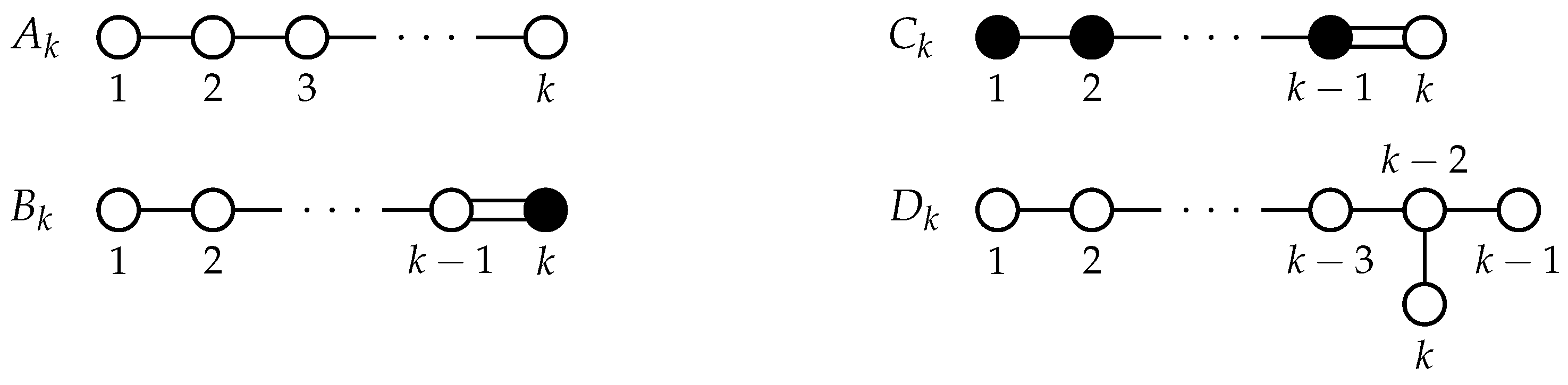
Suppose that there is exactly one connected component $U_1^{\vee }$ of the subgraph associated with the extended dual Dynkin diagram formed by the nodes corresponding to the zero coordinates ${\lambda }_i^{\sigma ,\varrho }$, $i\in {\widehat{I}}_n$ and the only zero coordinates are of the form ${\lambda }_0^{\sigma ,\varrho },\dots ,{\lambda }_j^{\sigma ,\varrho }$, $2\le j<n$. The Dynkin diagram of $U_1^{\vee }$ is according to Figure 2 of type $A_3$ for $j=2$ and of type $D_{j+1}$, otherwise. Thus, the value of Fourier–Weyl normalization functions are derived from Table 1 and defining relation (17) as

$$h_{\mathsf{\Gamma },M}\left(\lambda \right)=2,$$

(75)

$$h_M^{\vee }\left(\lambda \right)=2^j(j+1)!.$$

(76)

In this case, equivalence conditions (70) lead to the following restrictions on $k_i$, $i\in I_n$,

$$\frac{M}{2}-{\varrho }_n=k_1=k_2=\cdots =k_{j+1}>k_{j+2}>\cdots >k_n>-{\varrho }_n.$$

(77)

As discussed above, condition (71) is attained only for the symmetric cosine functions of types I and VII and for the symmetric sine functions of types II and VIII. Therefore, it follows from Table 2 and restrictions (77) that

$$h_{({\lambda }_1,\dots ,{\lambda }_n)}^{\mathrm{I},c}=h_{({\lambda }_1,\dots ,{\lambda }_n)}^{\mathrm{VII},c}=h_{({\lambda }_1,\dots ,{\lambda }_n)}^{\mathrm{II},s}=h_{({\lambda }_1,\dots ,{\lambda }_n)}^{\mathrm{VIII},s}=2^{j+1}{\left(\frac{M}{4}\right)}^n,$$

(78)

$$H_{({\lambda }_1,\dots ,{\lambda }_n)}=(j+1)!.$$

(79)

(iii)

If the only connected component $U_1^{\vee }$ is associated with the only zero magnified Kac coordinates of the form ${\lambda }_j^{\sigma ,\varrho }={\lambda }_{j+1}^{\sigma ,\varrho }=\cdots ={\lambda }_m^{\sigma ,\varrho }=0$ for $j>0$, $m<n$, the Dynkin diagram of $U_1^{\vee }$ corresponds, from Figure 2, to type $A_{m-j+1}$. According to Table 1, the Fourier–Weyl normalization function $h_M^{\vee }$ is evaluated as

$$h_M^{\vee }\left(\lambda \right)=(m-j+2)!$$

(80)

and defining relation (17) implies that the value of $h_{\mathsf{\Gamma },M}$ depends on whether the first two Kac coordinates coincide. The restrictions on the parameters $k_i$, $i\in I_n$ are deduced from equivalence conditions (70) as

$$\frac{M}{2}-{\varrho }_n\ge k_1>k_2>\cdots >k_j=k_{j+1}=\cdots =k_{m+1}>k_{m+2}>\cdots >k_n>-{\varrho }_n.$$

(81)

Assuming that the equality $M/2-{\varrho }_n=k_1$ holds, step (i) guarantees that the equivalent condition (71) is achieved only for the symmetric cosine functions of types I and VII and for the symmetric sine functions of types II and VIII. Therefore, Table 2 together with restrictions (81) assures that the values of trigonometric normalization functions are in this case given by (73). Otherwise, the trigonometric normalization functions are for any type of transform evaluated as

$$h_{({\lambda }_1,\dots ,{\lambda }_n)}^{\star ,c}=h_{({\lambda }_1,\dots ,{\lambda }_n)}^{\star ,s}={\left(\frac{M}{4}\right)}^n,\star \in \{\mathrm{I},\dots ,\mathrm{VIII}\}.$$

(82)

In both cases, it follows from restrictions (81) and definition (30) that

$$\begin{array}{cc}\hfill H_{({\lambda }_1,\dots ,{\lambda }_n)}& =(m-j+2)!.\hfill \end{array}$$

(83)

(iv)

If the only connected component $U_1^{\vee }$ is associated with the only zero magnified Kac coordinates of the form ${\lambda }_j^{\sigma ,\varrho }={\lambda }_{j+1}^{\sigma ,\varrho }=\cdots ={\lambda }_n^{\sigma ,\varrho }=0$ for $0<j\le n$, the Dynkin diagram of $U_1^{\vee }$ is according to Figure 2 of type $A_1$ for $j=n$, of type $C_2$ for $j=n-1$ and of type $B_{n-j+1}$ otherwise. Therefore, it results from Table 1 that

$$h_M^{\vee }\left(\lambda \right)=2^{n-j+1}(n-j+1)!$$

(84)

and the Fourier–Weyl normalization function $h_{\mathsf{\Gamma },M}$ depends, from defining relation (17), on the values of the first two Kac coordinates. Equivalence conditions (70) in this case guarantee the following restrictions:

$$\frac{M}{2}-{\varrho }_n\ge k_1>k_2>\cdots >k_j=k_{j+1}=\cdots =k_n=-{\varrho }_n.$$

(85)

Because ${\lambda }_n^{\sigma ,\varrho }=0$ is attained according to the ranges of the last magnified Kac coordinate (9) only if $\sigma =\mathfrak{1}$ and ${\varrho }_n=0$, Table 3 admits only the symmetric cosine transforms of the types $\mathrm{I},\mathrm{II},\mathrm{V}$ and $\mathrm{VI}$. Step (i) guarantees that the possible transforms reduce to the type $\mathrm{I}$ if the equality $M/2=k_1$ is valid. Therefore, it follows from Table 2 and restrictions (85) that the trigonometric normalization functions are, for $k_1\ne M/2$, evaluated as

$$h_{({\lambda }_1,\dots ,{\lambda }_n)}^{\mathrm{I},c}=h_{({\lambda }_1,\dots ,{\lambda }_n)}^{\mathrm{II},c}=h_{({\lambda }_1,\dots ,{\lambda }_n)}^{\mathrm{V},c}=h_{({\lambda }_1,\dots ,{\lambda }_n)}^{\mathrm{VI},c}=2^{n-j+1}{\left(\frac{M}{4}\right)}^n,$$

(86)

$$h_{(M/2,{\lambda }_2,\dots ,{\lambda }_n)}^{\mathrm{I},c}=2^{n-j+2}{\left(\frac{M}{4}\right)}^n,$$

(87)

$$H_{({\lambda }_1,\dots ,{\lambda }_n)}=H_{(M/2,{\lambda }_2,\dots ,{\lambda }_n)}=(n-j+1)!.$$

(88)

(v)

Assuming that the only zero magnified Kac coordinates are of the form ${\lambda }_0^{\sigma ,\varrho }={\lambda }_1^{\sigma ,\varrho }=0$ leads to the Dynkin diagram, denoted by $A_1\times A_1$, consisting of two connected components of type $A_1$. Thus, it follows from Table 1 and defining relations (18) and (17) that the Fourier–Weyl normalization functions are evaluated as

$$h_{\mathsf{\Gamma },M}\left(\lambda \right)=2,$$

(89)

$$h_M^{\vee }\left(\lambda \right)=4.$$

(90)

The following restrictions on the coordinates $k_i$, $i\in I_n$ are derived from equivalence conditions (70),

$$\frac{M}{2}-{\varrho }_n=k_1=k_2>k_3>\cdots >k_n>-{\varrho }_n.$$

(91)

Step (i) guarantees that the condition ${\lambda }_0^{\sigma ,\varrho }={\lambda }_1^{\sigma ,\varrho }$ is attained only for the symmetric cosine transforms of the types $\mathrm{I},\mathrm{VII}$ and for the symmetric sine transforms of the types $\mathrm{II},\mathrm{VIII}$. Table 2 and restrictions (91) produce that the values of the trigonometric normalization functions are given by

$$h_{({\lambda }_1,\dots ,{\lambda }_n)}^{\mathrm{I},c}=h_{({\lambda }_1,\dots ,{\lambda }_n)}^{\mathrm{VII},c}=h_{({\lambda }_1,\dots ,{\lambda }_n)}^{\mathrm{II},s}=h_{({\lambda }_1,\dots ,{\lambda }_n)}^{\mathrm{VIII},s}=4{\left(\frac{M}{4}\right)}^n,$$

(92)

$$H_{({\lambda }_1,\dots ,{\lambda }_n)}=2.$$

(93)

(vi)

Supposing that the subgraph of nodes associated with the zero Kac coordinates is formed by several connected components, then it combines blocks of nodes ${\tilde{U}}_1^{\vee },\dots ,{\tilde{U}}_p^{\vee }$ corresponding to the cases studied in steps (ii)–(v). Note that, if the block of two connected components from step (v) occurs, the total number of connected components equals $p+1$. Denoting by $h_M^{i,\vee }\left(\lambda \right)$ the value of the Fourier–Weyl normalization function (76), (80), (84) or (89) given by the step identified with the block ${\tilde{U}}_i^{\vee }$, defining relation (18) validates the identity

$$h_M^{\vee }\left(\lambda \right)=\prod _{i\in I_p}{h}_M^{i,\vee }\left(\lambda \right).$$

As in the previous steps, the value of $h_{\mathsf{\Gamma },M}\left(\lambda \right)$ depends on whether the first two Kac coordinates are equal or not. If $h_{({\lambda }_1,\dots ,{\lambda }_n)}^{\star ,c,i}$ and $h_{({\lambda }_1,\dots ,{\lambda }_n)}^{\star ,s,i}$ denote the value of trigonometric normalization functions (73), (78), (82), (86), (87), or (92) corresponding to the step of the block ${\tilde{U}}_i^{\vee }$, the definition of trigonometric normalization functions and steps (ii)–(v) imply that

$$\begin{array}{c}\hfill h_{({\lambda }_1,\dots ,{\lambda }_n)}^{\star ,c}=h_{\mathsf{\Gamma },M}{\left(\lambda \right)}^{1-p}\prod _{i\in I_p}{h}_{({\lambda }_1,\dots ,{\lambda }_n)}^{\star ,c,i},\\ \hfill h_{({\lambda }_1,\dots ,{\lambda }_n)}^{\star ,s}=h_{\mathsf{\Gamma },M}{\left(\lambda \right)}^{1-p}\prod _{i\in I_p}{h}_{({\lambda }_1,\dots ,{\lambda }_n)}^{\star ,s,i}.\end{array}$$

Denoting by $H_{({\lambda }_1,\dots ,{\lambda }_n)}^i$ the value of the trigonometric normalization function (79), (83), (88) or (93) depending on the step associated with the block ${\tilde{U}}_i^{\vee }$, it follows from definition (30) that

$$H_{({\lambda }_1,\dots ,{\lambda }_n)}=\prod _{i\in I_p}{H}_{({\lambda }_1,\dots ,{\lambda }_n)}^i.$$

For the antisymmetric cosine and sine label sets $D_N^{\star ,c,-}$ and $D_N^{\star ,s,-}$, the condition ${\lambda }_i^{\sigma ,\varrho }=0$ never occurs for some $i\in I_{n-1}$ and thus the identities (67) and (69) follow from steps (i), (iv), and (vi). □

5.2. Weight Functions

The goal of this section is to exactly connect the trigonometric point weight functions ${\epsilon }^{}\star ,c$ and ${\epsilon }^{}\star ,s$ with the Fourier–Weyl weight ${\epsilon }^{-}$function. The established one-to-one correspondence of the point sets from Theorem 2 is assumed. The following theorem presents explicitly the linking relations between the point weight functions.

Theorem 4.

The cosine and sine weight functions ${\epsilon }^{}\star ,c$ and ${\epsilon }^{}\star ,s$ and the Fourier–Weyl weight ${\epsilon }^{-}$functions are for $s=s_1{f}_1+\cdots +s_n{f}_n\in F_{Q^{\vee },M}^{\sigma }(\varrho ,{\nu }^{\vee })$ linked by the following expressions:

$${\epsilon }^{}{\star ,c}_{(s_1,\dots ,s_n)}{H}_{(s_1,\dots ,s_n)}^{-1}=\frac{{\epsilon }^{(}s)}{2^{n}n!},(s_1,\dots ,s_n)\in F_N^{\star ,c,+},$$

(94)

$${\epsilon }^{}{\star ,c}_{(s_1,\dots ,s_n)}=\frac{{\epsilon }^{(}s)}{2^{n}n!},(s_1,\dots ,s_n)\in F_N^{\star ,c,-},$$

(95)

$${\epsilon }^{}{\star ,s}_{(s_1,\dots ,s_n)}{H}_{(s_1,\dots ,s_n)}^{-1}=\frac{{\epsilon }^{(}s)}{2^{n}n!},(s_1,\dots ,s_n)\in F_N^{\star ,s,+},$$

(96)

$${\epsilon }^{}{\star ,s}_{(s_1,\dots ,s_n)}=\frac{{\epsilon }^{(}s)}{2^{n}n!},(s_1,\dots ,s_n)\in F_N^{\star ,s,-}.$$

(97)

Proof. 

Firstly, consider the points from the symmetric cosine and sine label sets $F_N^{\star ,c,+}$ and $F_N^{\star ,s,+}$ that, according to relations (55) and (57), are associated with the identity $\mathfrak{1}$ and long ${\sigma }^l$ sign homomorphisms point sets, respectively. The defining relation of Fourier–Weyl weight $\epsilon -$function assures that $\epsilon \left(s\right)$ differs from $2^{n}n!$ if and only if there exists $i\in {\widehat{I}}_n$ such that the corresponding magnified Kac coordinate $s_i^{\sigma ,\varrho }$ equals zero. This condition on the Kac coordinates is reformulated from equivalence conditions (62) for the coordinates $k_i$, $i\in I_n$, given by relations (60), as

$$\begin{array}{cc}{s}_0^{\sigma ,\varrho }=0\hfill & \iff k_1=\frac{M-{\nu }_n^{\vee }}{2},\hfill \\ s_i^{\sigma ,\varrho }=0\hfill & \iff k_i=k_{i+1},i\in I_{n-1},\hfill \\ s_n^{\sigma ,\varrho }=0\hfill & \iff k_n=-\frac{{\nu }_n^{\vee }}{2}.\hfill \end{array}$$

(98)

Conversely, taking any trigonometric point $(s_1,\dots ,s_n)$ from the symmetric cosine or sine point sets $F_N^{\star ,c,+}$ and $F_N^{\star ,s,+}$, the definitions of the trigonometric weight functions ${\epsilon }_{(s_1,\dots ,s_n)}^{\star ,c}{H}_{(s_1,\dots ,s_n)}^{-1}$ and ${\epsilon }_{(s_1,\dots ,s_n)}^{\star ,s}{H}_{(s_1,\dots ,s_n)}^{-1}$ guarantee that these functions vary from 1 only if the coordinate $k_i$ satisfies some equality among equivalence conditions (98) corresponding to some $i\in I_n$. In particular, the following steps are performed.

(i)

Suppose that there is exactly one connected component $U_1$ of the subgraph of the extended Dynkin diagram formed by the nodes corresponding to the zero coordinates $s_i^{\sigma ,\varrho }$, $i\in {\widehat{I}}_n$ and the only zero coordinates are of the form $s_0^{\sigma ,\varrho },\dots ,s_j^{\sigma ,\varrho }$, $0\le j<n$. The Dynkin diagram of $U_1$ is according to Figure 2 of type ${\mathcal{C}}_{j+1}$. Thus, the value of the Fourier–Weyl weight function is deduced from Table 1 and defining relation (20) as

$$\epsilon \left(s\right)=\frac{2^{n}n!}{2^{j+1}(j+1)!}.$$

(99)

In this case, equivalence conditions (98) force the following restrictions on $k_i$, $i\in I_n$,

$$\frac{M-{\nu }_n^{\vee }}{2}=k_1=k_2=\cdots =k_{j+1}>k_{j+2}>\cdots >k_n>-\frac{{\nu }_n^{\vee }}{2}.$$

(100)

The ranges of the first magnified Kac coordinate (12) and (13) admit the equality

$$s_0^{\sigma ,\varrho }=0$$

(101)

only for the cases $F_{Q^{\vee },M}^{\mathfrak{1}}(0,{\nu }^{\vee })$ and $F_{Q^{\vee },M}^{{\sigma }^l}\left(\frac{1}{2}{\omega }_n,{\nu }^{\vee }\right)$. Furthermore, according to the explicit forms of the Fourier–Weyl point sets (15), the cases $F_{Q^{\vee },M}^{\mathfrak{1}}(0,0)$ and $F_{Q^{\vee },M}^{\mathfrak{1}}(0,{\omega }_n^{\vee })$ permit condition (101) only for M even and odd and correspond in Table 3 to the symmetric cosine transforms of the types $\mathrm{I}$ and $\mathrm{VI}$, respectively. Similarly, the symmetric sine transforms are identified to be of the types $\mathrm{III}$ and $\mathrm{VIII}$ and Table 2, defining relation (30) and restrictions (100) validate

$${\epsilon }_{(s_1,\dots ,s_n)}^{\mathrm{I},c}={\epsilon }_{(s_1,\dots ,s_n)}^{\mathrm{VI},c}={\epsilon }_{(s_1,\dots ,s_n)}^{\mathrm{III},s}={\epsilon }_{(s_1,\dots ,s_n)}^{\mathrm{VIII},s}=\frac{1}{2^{j+1}},$$

(102)

$$H_{(s_1,\dots ,s_n)}^{-1}=\frac{1}{(j+1)!}.$$

(103)

(ii)

If the only connected component $U_1$ is associated with the only zero magnified Kac coordinates of the form $s_j^{\sigma ,\varrho }=s_{j+1}^{\sigma ,\varrho }=\cdots =s_m^{\sigma ,\varrho }=0$ for $j>0$, $m<n$, the Dynkin diagram of $U_1$ corresponds from Figure 2 to type $A_{m-j+1}$. Thus, the value of Fourier–Weyl weight function is derived from Table 1 and defining relation (20) as

$$\epsilon \left(s\right)=\frac{2^{n}n!}{(m-j+2)!}.$$

(104)

In this case, restrictions on $k_i$, $i\in I_n$ are deduced from equivalence conditions (98) as

$$\frac{M-{\nu }_n^{\vee }}{2}>k_1>\cdots >k_j=k_{j+1}=\cdots =k_{m+1}>k_{m+2}>\cdots >k_n>-\frac{{\nu }_n^{\vee }}{2}.$$

(105)

According to Table 2, defining relation (30) and restrictions (105), the trigonometric weight functions are evaluated for any type of transform as

$${\epsilon }_{(s_1,\dots ,s_n)}^{\star ,c}={\epsilon }_{(s_1,\dots ,s_n)}^{\star ,s}=1,\star \in \{\mathrm{I},\dots ,\mathrm{VIII}\},$$

(106)

$$H_{(s_1,\dots ,s_n)}^{-1}=\frac{1}{(m-j+2)!}.$$

(107)

(iii)

If the only connected component $U_1$ is associated with the only zero magnified Kac coordinates of the form $s_j^{\sigma ,\varrho }=s_{j+1}^{\sigma ,\varrho }=\cdots =s_n^{\sigma ,\varrho }=0$, $0<j\le n$, the Dynkin diagram of $U_1$ is of type ${\mathcal{C}}_{n-j+1}$. Therefore, the value of Fourier–Weyl weight function results from Table 1 and defining relation (20) as

$$\epsilon \left(s\right)=\frac{2^{n}n!}{2^{n-j+1}(n-j+1)!}.$$

(108)

Equivalence conditions (98) in this case guarantee the following restrictions on $k_i$, $i\in I_n$,

$$\frac{M-{\nu }_n^{\vee }}{2}>k_1>\cdots >k_j=k_{j+1}=\cdots =k_n=-\frac{{\nu }_n^{\vee }}{2}.$$

(109)

The ranges of the magnified Kac coordinates (14) together with explicit forms of the Fourier–Weyl point sets (15) admit the condition $s_n^{\sigma ,\varrho }=0$ only for the cases $F_{Q^{\vee },M}^{\mathfrak{1}}(0,0)$ and $F_{Q^{\vee },M}^{\mathfrak{1}}\left(\frac{1}{2}{\omega }_n,0\right)$ that correspond according to Table 3 to the symmetric cosine transforms of the types $\mathrm{I}$ and $\mathrm{III}$ for M even and $\mathrm{V}$ and $\mathrm{VII}$ for M odd. Table 2, defining relation (30), and restrictions (109) imply that the values of the trigonometric weight functions are given by

$${\epsilon }_{(s_1,\dots ,s_n)}^{\mathrm{I},c}={\epsilon }_{(s_1,\dots ,s_n)}^{\mathrm{III},c}={\epsilon }_{(s_1,\dots ,s_n)}^{\mathrm{V},c}={\epsilon }_{(s_1,\dots ,s_n)}^{\mathrm{VII},c}=\frac{1}{2^{n-j+1}},$$

(110)

$$H_{(s_1,\dots ,s_n)}^{-1}=\frac{1}{(n-j+1)!}.$$

(111)

(iv)

Suppose that the subgraph of nodes associated with the zero Kac coordinates is formed by several connected components $U_1,\dots ,U_p$, then each $U_i$, $i\in I_p$ identifies with one of the connected components from steps (i)–(iii). Denoting by ${\epsilon }_i\left(s\right)$ the value of the Fourier–Weyl weight function (99), (104) or (108) given by the step corresponding to $U_i$, defining relation (20) validates the identity

$$\epsilon \left(s\right)=\prod _{i\in I_p}{\epsilon }_i\left(s\right).$$

If ${\epsilon }_{(s_1,\dots ,s_n)}^{\star ,c,i}$ and ${\epsilon }_{(s_1,\dots ,s_n)}^{\star ,s,i}$ denote the value of trigonometric weight functions (102), (106) or (110) corresponding to the step of the component $U_i$, the definition of trigonometric weight functions and steps (i)–(iii) imply that

$$\begin{array}{cc}\hfill {\epsilon }_{(s_1,\dots ,s_n)}^{\star ,c}& =\prod _{i\in I_p}{\epsilon }_{(s_1,\dots ,s_n)}^{\star ,c,i},\hfill \\ \hfill {\epsilon }_{(s_1,\dots ,s_n)}^{\star ,s}& =\prod _{i\in I_p}{\epsilon }_{(s_1,\dots ,s_n)}^{\star ,s,i}.\hfill \end{array}$$

Denoting by $H_{(s_1,\dots ,s_n)}^i$, the value of the trigonometric weight function (103), (107) or (111) depending on the step associated with the component $U_i$, it follows from definition (30) that

$$H_{(s_1,\dots ,s_n)}=\prod _{i\in I_p}{H}_{(s_1,\dots ,s_n)}^i.$$

For the antisymmetric cosine and sine point sets $F_N^{\star ,c,-}$ and $F_N^{\star ,s,-}$, the condition $s_i^{\sigma ,\varrho }=0$ never occurs for some $i\in I_{n-1}$ and thus the identities (95) and (97) follow from steps (i), (iii), and (iv). □

6. Unitary Matrices of Discrete Transforms

The constructed one-to-one correspondences between the labels (44)–(47) and points (55)–(58) transfer the lexicographic ordering of the trigonometric point and label sets to their Fourier–Weyl counterparts. Assuming any such isomorphic order of the Fourier–Weyl sets ${\mathsf{\Lambda }}_{P,M}^{\sigma }(\varrho ,{\nu }^{\vee })$ and $F_{Q^{\vee },M}^{\sigma }(\varrho ,{\nu }^{\vee })$ and the corresponding trigonometric sets $D_N^{\star ,c,\pm }$, $D_N^{\star ,s,\pm }$, and $F_N^{\star ,c,\pm }$, $F_N^{\star ,s,\pm }$, the relations of the normalization and weight functions (66)–(69) and (94)–(97) guarantee the direct connection of the associated unitary transform matrices. Thus, the following theorem is obtained.

Theorem 5.

The unitary matrices (40)–(43) of the (anti)symmetric multivariate discrete trigonometric transforms are linked to the unitary matrices (22) of the generalized dual-root lattice Fourier–Weyl transforms of the series ${\mathcal{C}}_n$ by the following relations:

$$C_N^{\star ,+}={\mathbb{I}}_{Q^{\vee },M}^{\mathfrak{1}}(\varrho ,{\nu }^{\vee }),$$

(112)

$$C_N^{\star ,-}={\mathbb{I}}_{Q^{\vee },M}^{{\sigma }^s}(\varrho ,{\nu }^{\vee }),$$

(113)

$$S_N^{\star ,+}={\mathrm{i}}^n{\mathbb{I}}_{Q^{\vee },M}^{{\sigma }^l}(\varrho ,{\nu }^{\vee }),$$

(114)

$$S_N^{\star ,-}={\mathrm{i}}^n{\mathbb{I}}_{Q^{\vee },M}^{{\sigma }^e}(\varrho ,{\nu }^{\vee }),$$

(115)

where the correspondence of the type $\star \in \{\mathrm{I},\dots ,\mathrm{VIII}\}$ and magnifying factor $N\in \mathbb{N}$ with the magnifying factor $M\in \mathbb{N}$ and admissible shifts ϱ and ${\nu }^{\vee }$ is determined in Table 3.

As representative examples of the relations in Theorem 5 as well as explicit forms of the unitary transform matrices, the cases of types $\mathrm{II}$ and $\mathrm{VII}$ are presented in the following sections.

6.1. Type II

Setting the trigonometric magnifying factor $N=4$, the (anti)symmetric cosine sets of points $F_4^{\mathrm{II},c,+}$ and $F_4^{\mathrm{II},c,-}$, corresponding to the bivariate (anti)symmetric discrete cosine transforms of type II, consist of the following lexicographically ordered points:

$$\begin{array}{cc}\hfill F_4^{\mathrm{II},c,+}=& \left\{\left(\frac{1}{8},\frac{1}{8}\right),\left(\frac{3}{8},\frac{1}{8}\right),\left(\frac{3}{8},\frac{3}{8}\right),\left(\frac{5}{8},\frac{1}{8}\right),\left(\frac{5}{8},\frac{3}{8}\right),\left(\frac{5}{8},\frac{5}{8}\right),\left(\frac{7}{8},\frac{1}{8}\right),\left(\frac{7}{8},\frac{3}{8}\right),\left(\frac{7}{8},\frac{5}{8}\right),\left(\frac{7}{8},\frac{7}{8}\right)\right\},\hfill \\ \hfill F_4^{\mathrm{II},c,-}=& \left\{\left(\frac{3}{8},\frac{1}{8}\right),\left(\frac{5}{8},\frac{1}{8}\right),\left(\frac{5}{8},\frac{3}{8}\right),\left(\frac{7}{8},\frac{1}{8}\right),\left(\frac{7}{8},\frac{3}{8}\right),\left(\frac{7}{8},\frac{5}{8}\right)\right\}.\hfill \end{array}$$

The (anti)symmetric sine sets of points $F_4^{\mathrm{II},s,+}$ and $F_4^{\mathrm{II},s,-}$, corresponding to the bivariate (anti)symmetric discrete sine transforms of type II, coincide with the (anti)symmetric cosine sets of points $F_4^{\mathrm{II},c,+}$ and $F_4^{\mathrm{II},c,-}$,

$$F_4^{\mathrm{II},s,+}=F_4^{\mathrm{II},c,+},F_4^{\mathrm{II},s,-}=F_4^{\mathrm{II},c,-}.$$

From Theorem 2, the trigonometric sets of points determine the coordinates of the Fourier–Weyl sets of points $F_{Q^{\vee },8}^{\sigma }(0,{\omega }_2^{\vee })$, $\sigma \in \{\mathfrak{1},{\sigma }^s,{\sigma }^l,{\sigma }^e\}$ in the orthogonal $\mathcal{F}-$basis as

$$\begin{array}{cc}\hfill F_{Q^{\vee },8}^{\mathfrak{1}}(0,{\omega }_2^{\vee })=& \left\{s_1{f}_1+s_2{f}_2|(s_1,s_2)\in F_4^{\mathrm{II},c,+}\right\},\hfill \\ \hfill F_{Q^{\vee },8}^{{\sigma }^s}(0,{\omega }_2^{\vee })=& \left\{s_1{f}_1+s_2{f}_2|(s_1,s_2)\in F_4^{\mathrm{II},c,-}\right\},\hfill \\ \hfill F_{Q^{\vee },8}^{{\sigma }^l}(0,{\omega }_2^{\vee })=& \left\{s_1{f}_1+s_2{f}_2|(s_1,s_2)\in F_4^{\mathrm{II},s,+}\right\},\hfill \\ \hfill F_{Q^{\vee },8}^{{\sigma }^e}(0,{\omega }_2^{\vee })=& \left\{s_1{f}_1+s_2{f}_2|(s_1,s_2)\in F_4^{\mathrm{II},s,-}\right\}.\hfill \end{array}$$

As finite fragments of the shifted refined dual root lattice, the point sets $F_{Q^{\vee },8}^{\sigma }(0,{\omega }_2^{\vee })$, $\sigma \in \{\mathfrak{1},{\sigma }^s,{\sigma }^l,{\sigma }^e\}$ are plotted in Figure 3.

The (anti)symmetric cosine sets of labels $D_4^{\mathrm{II},c,+}$ and $D_4^{\mathrm{II},c,-}$, corresponding to the bivariate (anti)symmetric discrete cosine transforms of type II, consist of the following lexicographically ordered labels:

$$\begin{array}{cc}\hfill D_4^{\mathrm{II},c,+}=& \left\{\left(0,0\right),\left(1,0\right),\left(1,1\right),\left(2,0\right),\left(2,1\right),\left(2,2\right),\left(3,0\right),\left(3,1\right),\left(3,2\right),\left(3,3\right)\right\},\hfill \\ \hfill D_4^{\mathrm{II},c,-}=& \left\{\left(1,0\right),\left(2,0\right),\left(2,1\right),\left(3,0\right),\left(3,1\right),\left(3,2\right)\right\}.\hfill \end{array}$$

The (anti)symmetric sine sets of labels $D_4^{\mathrm{II},s,+}$ and $D_4^{\mathrm{II},s,-}$, corresponding to the bivariate (anti)symmetric discrete sine transforms of type II, contain the following lexicographically ordered labels:

$$\begin{array}{cc}\hfill D_4^{\mathrm{II},s,+}=& \left\{\left(1,1\right),\left(2,1\right),\left(2,2\right),\left(3,1\right),\left(3,2\right),\left(3,3\right),\left(4,1\right),\left(4,2\right),\left(4,3\right),\left(4,4\right)\right\},\hfill \\ \hfill D_4^{\mathrm{II},s,-}=& \left\{\left(2,1\right),\left(3,1\right),\left(3,2\right),\left(4,1\right),\left(4,2\right),\left(4,3\right)\right\}.\hfill \end{array}$$

From Theorem 1, the trigonometric sets of labels determine the coordinates of the Fourier–Weyl sets of labels ${\mathsf{\Lambda }}_{Q^{\vee },8}^{\sigma }(0,{\omega }_2^{\vee })$, $\sigma \in \{\mathfrak{1},{\sigma }^s,{\sigma }^l,{\sigma }^e\}$ in the orthogonal $\mathcal{F}-$basis,

$$\begin{array}{cc}\hfill {\mathsf{\Lambda }}_{Q^{\vee },8}^{\mathfrak{1}}(0,{\omega }_2^{\vee })=& \left\{{\lambda }_1{f}_1+{\lambda }_2{f}_2|({\lambda }_1,{\lambda }_2)\in D_4^{\mathrm{II},c,+}\right\},\hfill \\ \hfill {\mathsf{\Lambda }}_{Q^{\vee },8}^{{\sigma }^s}(0,{\omega }_2^{\vee })=& \left\{{\lambda }_1{f}_1+{\lambda }_2{f}_2|({\lambda }_1,{\lambda }_2)\in D_4^{\mathrm{II},c,-}\right\},\hfill \\ \hfill {\mathsf{\Lambda }}_{Q^{\vee },8}^{{\sigma }^l}(0,{\omega }_2^{\vee })=& \left\{{\lambda }_1{f}_1+{\lambda }_2{f}_2|({\lambda }_1,{\lambda }_2)\in D_4^{\mathrm{II},s,+}\right\},\hfill \\ \hfill {\mathsf{\Lambda }}_{Q^{\vee },8}^{{\sigma }^e}(0,{\omega }_2^{\vee })=& \left\{{\lambda }_1{f}_1+{\lambda }_2{f}_2|({\lambda }_1,{\lambda }_2)\in D_4^{\mathrm{II},s,-}\right\}.\hfill \end{array}$$

As fragments of the (non-shifted) weight lattice, the label sets ${\mathsf{\Lambda }}_{Q^{\vee },8}^{\sigma }(0,{\omega }_2^{\vee })$, $\sigma \in \{\mathfrak{1},{\sigma }^s,{\sigma }^l,{\sigma }^e\}$ are plotted in Figure 3.

The unitary transform matrices $C_4^{\mathrm{II},+}$ and $C_4^{\mathrm{II},-}$, corresponding to the (anti)symmetric bivariate discrete cosine transform of type II and coinciding with the unitary transform matrices ${\mathbb{I}}_{Q^{\vee },8}^{\mathfrak{1}}(0,{\omega }_2^{\vee })$ and ${\mathbb{I}}_{Q^{\vee },8}^{{\sigma }^s}(0,{\omega }_2^{\vee })$ of the generalized dual-root lattice Fourier–Weyl transforms, are calculated as

$$\begin{array}{cc}\hfill C_4^{\mathrm{II},+}& ={\mathbb{I}}_{Q^{\vee },8}^{\mathfrak{1}}(0,{\omega }_2^{\vee })=\left(\begin{array}{cccccccccc}0.250& 0.354& 0.250& 0.354& 0.354& 0.250& 0.354& 0.354& 0.354& 0.250\\ 0.462& 0.462& 0.191& 0.191& 0& -0.191& 0& -0.191& -0.462& -0.462\\ 0.427& 0.250& 0.073& -0.250& -0.104& 0.073& -0.604& -0.250& 0.250& 0.427\\ 0.354& 0& -0.354& 0& -0.500& -0.354& 0.500& 0& 0& 0.354\\ 0.462& -0.191& -0.191& -0.462& 0& 0.191& 0& 0.462& 0.191& -0.462\\ 0.250& -0.354& 0.250& -0.354& 0.354& 0.250& 0.354& -0.354& -0.354& 0.250\\ 0.191& -0.191& -0.462& 0.462& 0& 0.462& 0& -0.462& 0.191& -0.191\\ 0.250& -0.354& -0.250& 0.354& 0.354& -0.250& -0.354& 0.354& -0.354& 0.250\\ 0.191& -0.462& 0.462& 0.191& 0& -0.462& 0& -0.191& 0.462& -0.191\\ 0.073& -0.250& 0.427& 0.250& -0.604& 0.427& -0.104& 0.250& -0.250& 0.073\end{array}\right),\hfill \\ \\ \hfill C_4^{\mathrm{II},-}& ={\mathbb{I}}_{Q^{\vee },8}^{{\sigma }^s}(0,{\omega }_2^{\vee })=\left(\begin{array}{cccccc}-0.191& -0.462& -0.271& -0.653& -0.462& -0.191\\ -0.500& -0.500& 0& 0& 0.500& 0.500\\ -0.462& -0.191& -0.271& 0.653& -0.191& -0.462\\ -0.462& 0.191& 0.653& -0.271& 0.191& -0.462\\ -0.500& 0.500& 0& 0& -0.500& 0.500\\ -0.191& 0.462& -0.653& -0.271& 0.462& -0.191\\ \end{array}\right).\hfill \end{array}$$

The unitary transform matrices $S_4^{\mathrm{II},+}$ and $S_4^{\mathrm{II},-}$, corresponding to the (anti)symmetric bivariate discrete sine transform of type II and coinciding up to a sign with the unitary transform matrices ${\mathbb{I}}_{Q^{\vee },8}^{{\sigma }^l}(0,{\omega }_2^{\vee })$ and ${\mathbb{I}}_{Q^{\vee },8}^{{\sigma }^e}(0,{\omega }_2^{\vee })$ of the generalized dual-root lattice Fourier–Weyl transforms, are given as

$$\begin{array}{cc}\hfill S_4^{\mathrm{II},+}& =-{\mathbb{I}}_{Q^{\vee },8}^{{\sigma }^l}(0,{\omega }_2^{\vee })=\left(\begin{array}{cccccccccc}0.073& 0.250& 0.427& 0.250& 0.604& 0.427& 0.104& 0.250& 0.250& 0.073\\ 0.191& 0.462& 0.462& 0.191& 0& -0.462& 0& -0.191& -0.462& -0.191\\ 0.250& 0.354& 0.250& -0.354& -0.354& 0.250& -0.354& -0.354& 0.354& 0.250\\ 0.250& 0.354& -0.250& 0.354& -0.354& -0.250& 0.354& 0.354& 0.354& 0.250\\ 0.462& 0.191& -0.191& -0.462& 0& 0.191& 0& 0.462& -0.191& -0.462\\ 0.427& -0.250& 0.073& -0.250& 0.104& 0.073& 0.604& -0.250& -0.250& 0.427\\ 0.191& 0.191& -0.462& 0.462& 0& 0.462& 0& -0.462& -0.191& -0.191\\ 0.354& 0& -0.354& 0& 0.500& -0.354& -0.500& 0& 0& 0.354\\ 0.462& -0.462& 0.191& 0.191& 0& -0.191& 0& -0.191& 0.462& -0.462\\ 0.250& -0.354& 0.250& 0.354& -0.354& 0.250& -0.354& 0.354& -0.354& 0.250\end{array}\right),\hfill \\ \\ \hfill S_4^{\mathrm{II},-}& =-{\mathbb{I}}_{Q^{\vee },8}^{{\sigma }^e}(0,{\omega }_2^{\vee })=\left(\begin{array}{cccccc}-0.191& -0.462& -0.653& -0.271& -0.462& -0.191\\ -0.500& -0.500& 0& 0& 0.500& 0.500\\ -0.462& 0.191& -0.271& 0.653& 0.191& -0.462\\ -0.462& -0.191& 0.653& -0.271& -0.191& -0.462\\ -0.500& 0.500& 0& 0& -0.500& 0.500\\ -0.191& 0.462& -0.271& -0.653& 0.462& -0.191\end{array}\right).\hfill \end{array}$$

6.2. Type VII

Setting the trigonometric magnifying factor $N=4$, the (anti)symmetric cosine sets of points $F_4^{\mathrm{VII},c,+}$ and $F_4^{\mathrm{VII},c,-}$, which correspond to the bivariate (anti)symmetric discrete cosine transforms of type $\mathrm{VII}$, consist of the following lexicographically ordered points:

$$\begin{array}{cc}\hfill F_4^{\mathrm{VII},c,+}=& \left\{\left(0,0\right),\left(\frac{2}{7},0\right),\left(\frac{2}{7},\frac{2}{7}\right),\left(\frac{4}{7},0\right),\left(\frac{4}{7},\frac{2}{7}\right),\left(\frac{4}{7},\frac{4}{7}\right),\left(\frac{6}{7},0\right),\left(\frac{6}{7},\frac{2}{7}\right),\left(\frac{6}{7},\frac{4}{7}\right),\left(\frac{6}{7},\frac{6}{7}\right)\right\},\hfill \\ \hfill F_4^{\mathrm{VII},c,-}=& \left\{\left(\frac{2}{7},0\right),\left(\frac{4}{7},0\right),\left(\frac{4}{7},\frac{2}{7}\right),\left(\frac{6}{7},0\right),\left(\frac{6}{7},\frac{2}{7}\right),\left(\frac{6}{7},\frac{4}{7}\right)\right\}.\hfill \end{array}$$

The (anti)symmetric sine sets of points $F_4^{\mathrm{VII},s,+}$ and $F_4^{\mathrm{VII},s,-}$, corresponding to the bivariate (anti)symmetric discrete sine transforms of type $\mathrm{VII}$, contain the following lexicographically ordered points:

$$\begin{array}{cc}\hfill F_4^{\mathrm{VII},s,+}=& \left\{\left(\frac{2}{9},\frac{2}{9}\right),\left(\frac{4}{9},\frac{2}{9}\right),\left(\frac{4}{9},\frac{4}{9}\right),\left(\frac{6}{9},\frac{2}{9}\right),\left(\frac{6}{9},\frac{4}{9}\right),\left(\frac{6}{9},\frac{6}{9}\right),\left(\frac{8}{9},\frac{1}{9}\right),\left(\frac{8}{9},\frac{3}{9}\right),\left(\frac{8}{9},\frac{6}{9}\right),\left(\frac{8}{9},\frac{8}{9}\right)\right\},\hfill \\ \hfill F_4^{\mathrm{VII},s,-}=& \left\{\left(\frac{4}{9},\frac{2}{9}\right),\left(\frac{6}{9},\frac{2}{9}\right),\left(\frac{6}{9},\frac{4}{9}\right),\left(\frac{8}{9},\frac{1}{9}\right),\left(\frac{8}{9},\frac{3}{9}\right),\left(\frac{8}{9},\frac{6}{9}\right)\right\}.\hfill \end{array}$$

From Theorem 2, the trigonometric sets of points determine the coordinates of the Fourier–Weyl sets of points $F_{Q^{\vee },M}^{\sigma }(\frac{1}{2}{\omega }_2,0)$, $\sigma \in \{\mathfrak{1},{\sigma }^s,{\sigma }^l,{\sigma }^e\}$ in the orthogonal $\mathcal{F}-$basis as

$$\begin{array}{cc}\hfill F_{Q^{\vee },7}^{\mathfrak{1}}\left(\frac{1}{2}{\omega }_2,0\right)=& \left\{s_1{f}_1+s_2{f}_2|(s_1,s_2)\in F_4^{\mathrm{VII},c,+}\right\},\hfill \\ \hfill F_{Q^{\vee },7}^{{\sigma }^s}\left(\frac{1}{2}{\omega }_2,0\right)=& \left\{s_1{f}_1+s_2{f}_2|(s_1,s_2)\in F_4^{\mathrm{VII},c,-}\right\},\hfill \\ \hfill F_{Q^{\vee },9}^{{\sigma }^l}\left(\frac{1}{2}{\omega }_2,0\right)=& \left\{s_1{f}_1+s_2{f}_2|(s_1,s_2)\in F_4^{\mathrm{VII},s,+}\right\},\hfill \\ \hfill F_{Q^{\vee },9}^{{\sigma }^e}\left(\frac{1}{2}{\omega }_2,0\right)=& \left\{s_1{f}_1+s_2{f}_2|(s_1,s_2)\in F_4^{\mathrm{VII},s,-}\right\}.\hfill \end{array}$$

As finite fragments of the refined dual root lattice, the point sets $F_{Q^{\vee },7}^{\sigma }\left(\frac{1}{2}{\omega }_2,0\right)$, $\sigma \in \{\mathfrak{1},{\sigma }^s\}$ are plotted in Figure 4 and the point sets $F_{Q^{\vee },9}^{\sigma }\left(\frac{1}{2}{\omega }_2,0\right)$, $\sigma \in \{{\sigma }^l,{\sigma }^e\}$ are depicted in Figure 5.

The (anti)symmetric cosine sets of labels $D_4^{\mathrm{VII},c,+}$ and $D_4^{\mathrm{VII},c,-}$, corresponding to the bivariate (anti)symmetric discrete cosine transforms of type $\mathrm{VII}$, contain the following lexicographically ordered labels:

$$\begin{array}{cc}\hfill D_4^{\mathrm{VII},c,+}=& \left\{\left(\frac{1}{2},\frac{1}{2}\right),\left(\frac{3}{2},\frac{1}{2}\right),\left(\frac{3}{2},\frac{3}{2}\right),\left(\frac{5}{2},\frac{1}{2}\right),\left(\frac{5}{2},\frac{3}{2}\right),\left(\frac{5}{2},\frac{5}{2}\right),\left(\frac{7}{2},\frac{1}{2}\right),\left(\frac{7}{2},\frac{3}{2}\right),\left(\frac{7}{2},\frac{5}{2}\right),\left(\frac{7}{2},\frac{7}{2}\right)\right\},\hfill \\ \hfill D_4^{\mathrm{VII},c,-}=& \left\{\left(\frac{3}{2},\frac{1}{2}\right),\left(\frac{5}{2},\frac{1}{2}\right),\left(\frac{5}{2},\frac{3}{2}\right),\left(\frac{7}{2},\frac{1}{2}\right),\left(\frac{7}{2},\frac{3}{2}\right),\left(\frac{7}{2},\frac{5}{2}\right)\right\}.\hfill \end{array}$$

The (anti)symmetric sine sets of labels $D_4^{\mathrm{VII},s,+}$ and $D_4^{\mathrm{VII},s,-}$, which correspond to the bivariate (anti)symmetric discrete sine transforms of type $\mathrm{VII}$, coincide with the (anti)symmetric cosine label sets $D_4^{\mathrm{VII},c,+}$ and $D_4^{\mathrm{VII},c,-}$,

$$D_4^{\mathrm{VII},s,+}=D_4^{\mathrm{VII},c,+},D_4^{\mathrm{VII},s,-}=D_4^{\mathrm{VII},c,-}.$$

From Theorem 1, the trigonometric sets of labels determine the coordinates of the Fourier–Weyl sets of labels ${\mathsf{\Lambda }}_{Q^{\vee },M}^{\sigma }\left(\frac{1}{2}{\omega }_2,0\right)$, $\sigma \in \{\mathfrak{1},{\sigma }^s,{\sigma }^l,{\sigma }^e\}$ in the orthogonal $\mathcal{F}-$basis as

$$\begin{array}{cc}\hfill {\mathsf{\Lambda }}_{Q^{\vee },7}^{\mathfrak{1}}\left(\frac{1}{2}{\omega }_2,0\right)=& \left\{{\lambda }_1{f}_1+{\lambda }_2{f}_2|({\lambda }_1,{\lambda }_2)\in D_4^{\mathrm{VII},c,+}\right\},\hfill \\ \hfill {\mathsf{\Lambda }}_{Q^{\vee },7}^{{\sigma }^s}\left(\frac{1}{2}{\omega }_2,0\right)=& \left\{{\lambda }_1{f}_1+{\lambda }_2{f}_2|({\lambda }_1,{\lambda }_2)\in D_4^{\mathrm{VII},c,-}\right\},\hfill \\ \hfill {\mathsf{\Lambda }}_{Q^{\vee },9}^{{\sigma }^l}\left(\frac{1}{2}{\omega }_2,0\right)=& \left\{{\lambda }_1{f}_1+{\lambda }_2{f}_2|({\lambda }_1,{\lambda }_2)\in D_4^{\mathrm{VII},s,+}\right\},\hfill \\ \hfill {\mathsf{\Lambda }}_{Q^{\vee },9}^{{\sigma }^e}\left(\frac{1}{2}{\omega }_2,0\right)=& \left\{{\lambda }_1{f}_1+{\lambda }_2{f}_2|({\lambda }_1,{\lambda }_2)\in D_4^{\mathrm{VII},s,-}\right\}.\hfill \end{array}$$

As finite fragments of the shifted weight lattice, the label sets ${\mathsf{\Lambda }}_{Q^{\vee },7}^{\sigma }\left(\frac{1}{2}{\omega }_2,0\right)$, $\sigma \in \{\mathfrak{1},{\sigma }^s\}$ are plotted in Figure 4 and the label sets ${\mathsf{\Lambda }}_{Q^{\vee },9}^{\sigma }\left(\frac{1}{2}{\omega }_2,0\right)$, $\sigma \in \{{\sigma }^l,{\sigma }^e\}$ are depicted in Figure 5.

The unitary transform matrices $C_4^{\mathrm{VII},+}$ and $C_4^{\mathrm{VII},-}$, corresponding to the (anti)symmetric bivariate discrete cosine transforms of type $\mathrm{VII}$ and coinciding with the unitary matrices ${\mathbb{I}}_{Q^{\vee },7}^{\mathfrak{1}}\left(\frac{1}{2}{\omega }_2,0\right)$ and ${\mathbb{I}}_{Q^{\vee },7}^{{\sigma }^s}\left(\frac{1}{2}{\omega }_2,0\right)$ of the generalized dual-root lattice Fourier–Weyl transforms, are given as

$$\begin{array}{cc}\hfill C_4^{\mathrm{VII},+}& ={\mathbb{I}}_{Q^{\vee },7}^{\mathfrak{1}}\left(\frac{1}{2}{\omega }_2,0\right)=\left(\begin{array}{cccccccccc}0.286& 0.515& 0.464& 0.356& 0.454& 0.222& 0.127& 0.162& 0.112& 0.028\\ 0.404& 0.454& 0.162& -0.112& -0.385& -0.454& -0.162& -0.293& -0.337& -0.112\\ 0.286& 0.127& 0.028& -0.515& -0.162& 0.464& -0.356& -0.112& 0.454& 0.222\\ 0.404& 0.112& -0.454& 0.162& -0.337& -0.112& 0.454& 0.385& 0.293& 0.162\\ 0.404& -0.162& -0.112& -0.454& 0.293& 0.162& 0.112& 0.337& -0.385& -0.454\\ 0.286& -0.356& 0.222& -0.127& 0.112& 0.028& 0.515& -0.454& -0.162& 0.464\\ 0.286& -0.028& -0.515& 0.464& 0.112& 0.356& -0.222& -0.454& -0.162& -0.127\\ 0.286& -0.222& -0.127& 0.028& 0.454& -0.515& -0.464& 0.162& 0.112& 0.356\\ 0.286& -0.464& 0.356& 0.222& -0.162& -0.127& -0.028& -0.112& 0.454& -0.515\\ 0.143& -0.286& 0.286& 0.286& -0.404& 0.286& -0.286& 0.404& -0.404& 0.286\end{array}\right),\hfill \\ \\ \hfill C_4^{\mathrm{VII},-}& ={\mathbb{I}}_{Q^{\vee },7}^{{\sigma }^s}\left(\frac{1}{2}{\omega }_2,0\right)=\left(\begin{array}{cccccc}-0.274& -0.616& -0.543& -0.342& -0.349& -0.108\\ -0.616& -0.342& 0.108& 0.274& 0.543& 0.349\\ -0.342& 0.274& -0.349& 0.616& -0.108& -0.543\\ -0.543& 0.108& 0.616& -0.349& -0.274& -0.342\\ -0.349& 0.543& -0.274& -0.108& -0.342& 0.616\\ -0.108& 0.349& -0.342& -0.543& 0.616& -0.274\end{array}\right).\hfill \end{array}$$

The unitary transform matrices $S_4^{\mathrm{VII},+}$ and $S_4^{\mathrm{VII},-}$, corresponding to the (anti)symmetric bivariate discrete sine transforms of type $\mathrm{VII}$ and coinciding up to a sign with the unitary matrices ${\mathbb{I}}_{Q^{\vee },9}^{{\sigma }^l}\left(\frac{1}{2}{\omega }_2,0\right)$ and ${\mathbb{I}}_{Q^{\vee },9}^{{\sigma }^e}\left(\frac{1}{2}{\omega }_2,0\right)$ of the generalized dual-root lattice Fourier–Weyl transforms, are calculated as

$$\begin{array}{cc}\hfill S_4^{\mathrm{VII},+}& =-{\mathbb{I}}_{Q^{\vee },9}^{{\sigma }^l}\left(\frac{1}{2}{\omega }_2,0\right)=\left(\begin{array}{cccccccccc}0.052& 0.138& 0.184& 0.186& 0.350& 0.333& 0.212& 0.398& 0.536& 0.431\\ 0.186& 0.379& 0.350& 0.333& 0.333& 0& 0.247& 0.132& -0.333& -0.536\\ 0.333& 0.471& 0.333& 0& 0& 0& -0.471& -0.471& 0& 0.333\\ 0.212& 0.229& -0.138& 0.247& -0.379& -0.471& 0.529& 0.034& -0.132& 0.398\\ 0.536& 0.247& -0.186& -0.333& -0.333& 0& -0.132& 0.379& 0.333& -0.350\\ 0.431& -0.212& 0.052& -0.536& 0.186& 0.333& 0.398& -0.138& -0.350& 0.184\\ 0.138& 0.034& -0.398& 0.379& -0.132& 0.471& 0.229& -0.529& 0.247& -0.212\\ 0.350& -0.132& -0.536& 0.333& 0.333& 0& -0.379& 0.247& -0.333& 0.186\\ 0.398& -0.529& 0.212& 0.132& 0.247& -0.471& 0.034& -0.229& 0.379& -0.138\\ 0.184& -0.398& 0.431& 0.350& -0.536& 0.333& -0.138& 0.212& -0.186& 0.052\end{array}\right),\hfill \\ \\ \hfill S_4^{\mathrm{VII},-}& =-{\mathbb{I}}_{Q^{\vee },9}^{{\sigma }^e}\left(\frac{1}{2}{\omega }_2,0\right)=\left(\begin{array}{cccccc}-0.116& -0.333& -0.333& -0.511& -0.626& -0.333\\ -0.333& -0.511& -0.116& -0.333& 0.333& 0.626\\ -0.511& -0.333& -0.333& 0.626& 0.116& -0.333\\ -0.333& -0.116& 0.626& -0.333& 0.333& -0.511\\ -0.626& 0.333& 0.333& 0.116& -0.511& 0.333\\ -0.333& 0.626& -0.511& -0.333& 0.333& -0.116\end{array}\right).\hfill \end{array}$$

7. Conclusions

• The presented link of the generalized root-lattice Fourier–Weyl transforms related to the crystallographic series ${\mathcal{C}}_n$ to the (anti)symmetric trigonometric transforms provides significant advantages for the further development and method transfer in both directions. The analogous form of the label and point sets in the trigonometric approach enables embedding of both ${\mathcal{C}}_n$ transform sets by a common choice of the $\mathcal{F}-$basis (35). Besides comparison of the label and point sets in Theorems 1 and 2, the more challenging evaluation of the ${\mathcal{C}}_n$ weight and normalization functions relies on the Coxeter–Dynkin diagrams counting algorithms [14]. The achieved results of the extended (dual) Coxeter–Dynkin diagram analysis in Theorems 3 and 4 demonstrate feasible explicit forms of the Fourier–Weyl weight and normalization functions that are independent on Lie theory. Formulation of similarly directly structured final forms encoding the $A_n$, $B_n$ and $D_n$ transforms poses an open problem.
• The family of 32 cubature formulas for multivariate numerical integration belongs to the class of the Chebyshev polynomial methods that are obtained utilizing the present (anti)symmetric trigonometric transforms [9,10]. Among the cubature formulas of this family, eight types lead to the Gaussian rules with the highest precision. Migration of the multivariate Chebyshev polynomials [5] via the functional substitution (36) together with the Chebyshev nodes and weight functions conversions straightforwardly generates cubature formulas in the Lie theoretical setting [8,26]. Such direct comparison indicates the presence of other Gaussian rules attached to the generalized root-lattice Fourier–Weyl transforms of the remaining crystallographic root systems. The presented correspondence between the discrete transforms allows for further research pertaining to the Lebesgue constant estimates of the polynomial cubatures in both frameworks.
• Defined by relations analogous to the trigonometric symmetrizations (31)–(34), the multivariate antisymmetric and symmetric exponential functions represent distinct variants of the $S_n$ induced special functions [40]. A similar form of the point and label sets of the discrete Fourier transforms associated with the (anti)symmetric exponential functions and the present ${\mathcal{C}}_n$ root-lattice Fourier–Weyl transforms signals the existence of novel types of orbit functions and induced discrete transforms attached to all crystallographic root systems. Successful interpolation tests demonstrated for both 2D and 3D cases [2,41] of the (anti)symmetric exponential Fourier transforms suggest the transforms’ significant application potential. Moreover, the one-parameter variable position of the point sets relative to the triangular fundamental domain of the (anti)symmetric exponential functions [2] reveals different types of admissible shifts of the Weyl (sub)group invariant lattices [4,18].
• The research toward unique types of symmetrized multivariate exponential functions, invariant with respect to the even subgroups of the Weyl groups, produces the even orbit $E-$functions [42] together with the ten types of the even dual weight lattice Fourier–Weyl transforms [43]. Taking into account the alternating subgroup of the permutation group $S_n$, the trigonometric adaptation of the $E-$functions results in both alternating trigonometric and exponential functions as well as the associated discrete Fourier transforms [44,45]. According to the currently assembled correspondence between the functions and discrete transforms, the link between the alternating trigonometric functions and the ${\mathcal{C}}_n$ series $E-$functions is expected. Even though their existence is strongly indicated by the presently obtained connection, the exact forms of the (dual) root-lattice Fourier–Weyl $E-$transforms have not yet been derived for any case. The (dual) root-lattice Fourier–Weyl $E-$transforms along with their ties to the alternating trigonometric and exponential functions deserve further study.

References

- Klimyk, A.; Patera, J. (Anti)symmetric multivariate trigonometric functions and corresponding Fourier transforms. J. Math. Phys. 2007, 48, 093504. [Google Scholar] [CrossRef]
- Hrivnák, J.; Patera, J. Two-dimensional symmetric and antisymmetric generalizations of exponential and cosine functions. J. Math. Phys. 2010, 51, 023515. [Google Scholar] [CrossRef]
- Hrivnák, J.; Motlochová, L. Dual-root lattice discretization of Weyl orbit functions. J. Fourier Anal. Appl. 2019, 25, 2521–2569. [Google Scholar] [CrossRef]
- Czyżycki, T.; Hrivnák, J.; Motlochová, L. Generalized Dual-Root Lattice Transforms of Affine Weyl Groups. Symmetry 2020, 12, 1018. [Google Scholar] [CrossRef]
- Hrivnák, J.; Motlochová, L. On connecting Weyl-orbit functions to Jacobi polynomials and multivariate (anti)symmetric trigonometric functions. Acta Polytech. 2016, 56, 283–290. [Google Scholar] [CrossRef]
- Klimyk, A.; Patera, J. Orbit functions. SIGMA 2006, 2, 006. [Google Scholar]
- Klimyk, A.; Patera, J. Antisymmetric orbit functions. SIGMA 2007, 3, 023. [Google Scholar] [CrossRef]
- Moody, R.V.; Motlochová, L.; Patera, J. Gaussian cubature arising from hybrid characters of simple Lie groups. J. Fourier Anal. Appl. 2014, 20, 1257–1290. [Google Scholar] [CrossRef]
- Hrivnák, J.; Motlochová, L. Discrete transforms and orthogonal polynomials of (anti)symmetric multivariate cosine functions. SIAM J. Numer. Anal. 2010, 51, 073509. [Google Scholar] [CrossRef]
- Brus, A.; Hrivnák, J.; Motlochová, L. Discrete Transforms and Orthogonal Polynomials of (Anti)symmetric Multivariate Sine Functions. Entropy 2018, 20, 938. [Google Scholar] [CrossRef]
- Britanak, V.; Rao, K.; Yip, P. Discrete Cosine and Sine Transforms: General Properties, Fast Algorithms and Integer Approximations; Elsevier: Amsterdam, The Netherlands, 2007. [Google Scholar]
- Hrivnák, J.; Motlochová, L.; Patera, J. Two-dimensional symmetric and antisymmetric generalizations of sine functions. J. Math. Phys. 2010, 51, 073509. [Google Scholar] [CrossRef]
- van Diejen, J.F.; Emsiz, E. Discrete Fourier transform associated with generalized Schur polynomials. Proc. Am. Math. Soc. 2018, 146, 3459–3472. [Google Scholar] [CrossRef]
- Hrivnák, J.; Patera, J. On discretization of tori of compact simple Lie groups. J. Phys. A Math. Theor. 2009, 42, 385208. [Google Scholar] [CrossRef]
- Hrivnák, J.; Motlochová, L.; Patera, J. On discretization of tori of compact simple Lie groups II. J. Phys. A Math. Theor. 2012, 45, 255201. [Google Scholar]
- Li, H.; Xu, Y. Discrete Fourier analysis on fundamental domain and simplex of Ad lattice in d-variables. J. Fourier Anal. Appl. 2010, 16, 383–433. [Google Scholar]
- Hrivnák, J.; Walton, M.A. Weight-Lattice Discretization of Weyl-Orbit Functions. J. Math. Phys. 2016, 57, 083512. [Google Scholar] [CrossRef]
- Czyżycki, T.; Hrivnák, J. Generalized discrete orbit function transforms of affine Weyl groups. J. Math. Phys. 2014, 55, 113508. [Google Scholar] [CrossRef]
- Strang, G. The discrete cosine transform. SIAM Rev. 1999, 41, 135–147. [Google Scholar] [CrossRef]
- Wen, W.; Kajínek, O.; Khatibi, S.; Chadzitaskos, G. A Common Assessment Space for Different Sensor Structures. Sensors 2019, 19, 568. [Google Scholar] [CrossRef]
- Moody, R.V.; Patera, J. Orthogonality within the families of C-, S-, and E-functions of any compact semisimple Lie group. SIGMA 2006, 2, 076. [Google Scholar] [CrossRef]
- Hrivnák, J.; Myronova, M.; Patera, J. Central Splitting of A2 Discrete Fourier–Weyl Transforms. Symmetry 2020, 12, 1828. [Google Scholar] [CrossRef]
- Berens, H.; Schmid, H.J.; Xu, Y. Multivariate Gaussian cubature formulae. Arch. Math. 1995, 64, 26–32. [Google Scholar] [CrossRef]
- Heckman, G.; Schlichtkrull, H. Harmonic Analysis and Special Functions on Symmetric Spaces; Academic Press Inc.: San Diego, CA, USA, 1994. [Google Scholar]
- Koornwinder, T.H. Two-variable analogues of the classical orthogonal polynomials. Theory Appl. Spec. Funct. 1975, 435–495. [Google Scholar]
- Moody, R.V.; Patera, J. Cubature formulae for orthogonal polynomials in terms of elements of finite order of compact simple Lie groups. Adv. Appl. Math. 2011, 47, 509–535. [Google Scholar] [CrossRef]
- Hrivnák, J.; Motlochová, L.; Patera, J. Cubature formulas of multivariate polynomials arising from symmetric orbit functions. Symmetry 2016, 8, 63. [Google Scholar] [CrossRef]
- Hrivnák, J.; Motlochová, L. Discrete cosine and sine transforms generalized to honeycomb lattice. J. Math. Phys. 2018, 59, 063503. [Google Scholar] [CrossRef]
- Hrivnák, J.; Motlochová, L. Graphene Dots via Discretizations of Weyl-Orbit Functions. In Lie Theory and Its Applications in Physics, Varna, Bulgaria, June 2019; Dobrev, V., Ed.; Springer: Singapore, 2020; pp. 407–413. [Google Scholar]
- Cserti, J.; Tichy, G. A simple model for the vibrational modes in honeycomb lattices. Eur. J. Phys. 2004, 25, 723–736. [Google Scholar] [CrossRef][Green Version]
- Güçlü, A.D.; Potasz, P.; Korkusinski, M.; Hawrylak, P. Graphene Quantum Dots; Springer: Berlin, Germany, 2014. [Google Scholar]
- Drissi, L.B.; Saidi, E.H.; Bousmina, M. Graphene, Lattice Field Theory and Symmetries. J. Math. Phys. 2011, 52, 022306. [Google Scholar] [CrossRef]
- Siddeq, M.M.; Rodrigues, M.A. DCT and DST Based Image Compression for 3D Reconstruction. 3D Res. 2017, 8, 5. [Google Scholar] [CrossRef]
- Çapoğlu, I.R.; Taflove, A.; Backman, V. Computation of tightly-focused laser beams in the FDTD method. Opt. Express 2013, 21, 87–101. [Google Scholar] [CrossRef]
- Crivellini, A.; D’Alessandro, V.; Bassi, F. High-order discontinuous Galerkin solutions of three-dimensional incompressible RANS equations. Comput. Fluids 2013, 81, 122–133. [Google Scholar] [CrossRef]
- Young, J.C.; Gedney, S.D.; Adams, R.J. Quasi-Mixed-Order Prism Basis Functions for Nyström-Based Volume Integral Equations. IEEE Trans. Magn. 2012, 48, 2560–2566. [Google Scholar] [CrossRef]
- Chernyshenko, D.; Fangohr, H. Computing the demagnetizing tensor for finite difference micromagnetic simulations via numerical integration. J. Magn. Magn. Mater. 2015, 381, 440–445. [Google Scholar] [CrossRef]
- Bourbaki, N. Groupes et Algèbres de Lie, Chapiters IV, V, VI; Hermann: Paris, France, 1968. [Google Scholar]
- Humphreys, J.E. Reflection Groups and Coxeter Groups; Cambridge Studies in Advanced Mathematics 29; Cambridge University Press: Cambridge, UK, 1990. [Google Scholar]
- Klimyk, A.U.; Patera, J. (Anti)symmetric multivariate exponential functions and corresponding Fourier transforms. J. Phys. A Math. Theor. 2007, 40, 10473–10489. [Google Scholar] [CrossRef]
- Bezubik, A.; Hrivnák, J.; Patera, J.; Pošta, S. Three–variable symmetric and antisymmetric exponential functions and orthogonal polynomials. Math. Slovac. 2017, 67, 427–446. [Google Scholar] [CrossRef]
- Klimyk, A.U.; Patera, J. E-orbit functions. SIGMA 2008, 4, 002. [Google Scholar]
- Hrivnák, J.; Juránek, M. On E-Discretization of Tori of Compact Simple Lie Groups. II. J. Math. Phys. 2017, 58, 103504. [Google Scholar] [CrossRef]
- Klimyk, A.U.; Patera, J. Alternating multivariate trigonometric functions and corresponding Fourier transforms. J. Phys. A Math. Theor. 2008, 41, 145205. [Google Scholar] [CrossRef]
- Klimyk, A.; Patera, J. Alternating Group and Multivariate Exponential Functions. In Groups and Symmetries, From Neolithic Scots to John McKay; Harnad, J., Winternitz, P., Eds.; American Mathematical Society: Providence, RI, USA, 2009; pp. 233–246. [Google Scholar]