Abstract
Proposing new strategies to improve the optimization performance of differential evolution (DE) is an important research study. The jSO algorithm was the announced winner of the Congress on Evolutionary Computation (CEC) 2017 competition on numerical optimization, and is the state-of-the-art algorithm in the SHADE (Success-History based Adaptive Differential Evolution) algorithm series. However, the jSO algorithm converges prematurely in the search space with different dimensions and is prone to falling into local optimum during evolution, as well as the problem of decreasing population diversity. In this paper, a modified jSO algorithm (MjSO) is proposed which is based on cosine similarity with parameter adaptation and a novel opposition-based learning restart mechanism incorporated with symmetry to address the above problems, respectively. Moreover, it is well known that parameter setting has a significant impact on the performance of the algorithm and the search process can be divided into two symmetrical parts. Hence, a parameter control strategy based on a symmetric search process is introduced in the MjSO. The effectiveness of these designs is supported by presenting a population clustering analysis, along with a population diversity measure to evaluate the performance of the proposed algorithm, three state-of-the-art DE variant algorithms (EBLSHADE, ELSHADE-SPACMA, and SALSHADE-cnEPSin) and two original algorithms (jSO and LSHADE) are compared with it, for solving 30 CEC’17 benchmark functions and three classical engineering design problems. The experimental results and analysis reveal that the proposed algorithm can outperform other competitions in terms of the convergence speed and the quality of solutions. Promisingly, the proposed method can be treated as an effective and efficient auxiliary tool for more complex optimization models and scenarios.
1. Introduction
In the real world, there are many engineering optimization problems that need to be solved. The design cost problems in engineering have some practical constraints and one or more objective functions [1]. These engineering problems often demand methods to find optimum from a large number of available solutions, without wasting efforts in searching sub-optimal regions. Because of the large number of these problems and their practical application value, it has become a research hotspot in recent years. These problems are characterized mainly by their large scale and high difficulty. When the traditional optimization algorithm solves such a large-scale problem, it has certain inherent drawbacks, such as local optimal stagnation and derivation of the search space. Therefore, much attention has been paid to stochastic optimization methods [2] in recent decades [3,4]. Stochastic optimization algorithms can avoid the derivation of the mathematical model in that they only adjust the inputs and monitor the outputs of a given system for objective outputs and treat the optimization task as a black box [5]. In addition, stochastic optimization algorithms can solve optimization tasks randomly [6], which means that they have intrinsic superiority over conventional optimization algorithms in the capability of local optimal avoidance. Based on the number of solutions generated at each iteration optimization during the whole process, stochastic optimization algorithms can be divided into population-based algorithms, which generate many random solutions and promote them during the full optimization, and individual-based algorithms, which generate only one candidate solution throughout optimization.
Numerous stochastic optimization algorithms have been proposed based on evolutionary phenomena, swarm-based intelligence techniques, physical rules, and human-related concepts. Evolutionary algorithms include genetic algorithm (GA) [7], particle swarm optimization (PSO) [8], differential evolution (DE) [9], and evolutionary strategy (ES) [10]. Swarm-based intelligence algorithms usually simulate living beings’ behavior of social hierarchy, cooperation, and collective, and then mathematically abstract optimization models for problems to be optimized.
The differential evolution (DE) algorithm was proposed by Storn and Price [9] in 1995, and this laid the foundation for a series of successful continuous optimization algorithms. Literature [11] summarizes the extensive research fields focused on DE in recent years. The algorithms based on DE [12,13,14,15,16,17,18,19,20,21,22,23,24,25,26] have gained very high rankings in various competitions held annually at the IEEE (Institute of Electrical and Electronics Engineers) Congress on Evolutionary Computation (CEC). Therefore, DE-based algorithms are generally considered to be an effective and popular population-based evolutionary algorithm for single-objective continuous optimization problems [27,28].
In recent years, many modified algorithms based on DE algorithms have been derived [29]. In addition to combining DE with other algorithms, the main research modifications of DE include the exploitation of mutation strategies to control the movement of individuals and the adaptive modification of the DE control parameters during operation. SHADE is an adaptive DE that combines parameter adaptation based on the success history with one of the most advanced DE algorithms [30]. LSHADE further expands SHADE through linear population size reduction (LPSR), thus continuously reducing the population size using linear functions [31]. The jSO algorithm, which mainly has a new weighted version of the mutation strategy and some parameter settings, is an improved variant of the LSHADE algorithm [32]. ELSHADE-SPACMA is an improved method based on LSHADE-SPACMA. In LSHADE-SPACMA, the value of p used to control the degree of the greed of the mutant strategy is constant, while in ELSHADE-SPACMA, the value of p is dynamic. The performance of ELSHADE-SPACMA was further improved by integrating another directed mutation strategy into the hybridization framework [33,34]. The improved SALSHADE algorithm with global optimization linearly reduces the scaling factor and exponentially reduces the crossover rate and final Levy distribution step size to adapt to the improvement of the frequency component [35]. These classical algorithms will be reviewed in Section 2.
Furthermore, one of the disadvantages of differential evolutionary algorithms is the loss of population diversity. Therefore, the algorithm may prematurely converge to the local optimum. A good algorithm needs to have high enough population diversity in the early stage of the evolutionary process while reducing the population diversity to improve the convergence rate in the late stage. In order to solve the problems of premature convergence and population stagnation, Ming Yang et al. [36] study the adaptability of the population diversity in dimensions and a mechanism called automatically enhanced population diversity (AEPD) was proposed to automatically enhance the population diversity. Cheng Hongtan et al. [37] focus on controlling the value of the search parameter P. In his proposal, after he normalized the diversity of the population, each individual would select its unique search area according to the diversity conditions. Jing-zhong Wang et al. [38] proposed a variation strategy for a differential evolutionary algorithm (DE) with a fuzzy inference system (FIS), which enables the FIS to have well-controlled population diversity performance by controlling the ratio of the variation with respect to the globally optimal individual. All previously mentioned algorithms share the same idea of balancing between exploration and exploitation abilities, and they try to achieve it in various ways, but there is a general issue that they cannot maintain a long exploration phase or the ability to jump out of local optimum.
Nevertheless, many improved algorithms based on DE algorithms have made great progress in engineering problems. Xiaoyu He et al. [39] proposed a novel DE variant with covariance matrix self-adaptation, which produces a good solution for solving three classic constrained engineering design problems (pressure vessel design problem, tension/compression spring design problem and welded beam design problem). Noor H. Awad et al. [40] introduced an effective surrogate model to assist the differential evolution algorithm to generate competitive solutions during the search process and solved the two engineering design problems of welded beams and pressure vessels. At the same time, the improved algorithm fused with the DE algorithm has also achieved good performance in solving engineering problems. K.R. Subhashini et al. [41] integrated the basic animal migration optimization (AMO) algorithm with the DE algorithm and applied it to engineering problems. The result is significantly better than the original algorithm AMO.
Therefore, this study proposes a modified jSO algorithm to solve engineering problem. The MjSO algorithm uses a novel parameter adaptive mechanism based on cosine similarity instead of the original scaling factor and crossover rate with the weighted mean adaptive mechanism and adopts a parameter control strategy based on a symmetric search process. Thus, it can maintain a high population diversity and a longer exploration phase. In addition, in order to jump out of the local optimum, a novel opposition-based learning restart mechanism is applied. Finally, abundant experiments on 30 unconstrained benchmark functions [42], and 3 constrained engineering problems are carried out to demonstrate the superiority of MjSO algorithm. The experimental results show that the proposed MjSO algorithm can obtain more persuasive optima results than other optimization algorithms on unconstrained benchmark functions and achieve less cost engineering design results than other algorithms on constrained engineering problems.
The rest of this article is arranged as follows: in Section 2, several of the more famous DE variants are reviewed. The MjSO algorithm is described in detail in Section 3. Section 4 describes the experimental setup. Section 5 presents the analysis of the experimental results. The proposed MjSO algorithm for engineering problems is conducted in Section 6. Finally, the conclusion is given in Section 7.
2. Related Work
In this section, several of the state-of-the-art DE variants will be reviewed, including JADE [43], SHADE [30], LSHADE [31], iLSHADE [44], and jSO [32], because our proposed MjSO algorithm is a further extension of these algorithms. In addition, these algorithms provide a clear idea for the exploitation of DE. By introducing these state-of-the-art DE variants, researchers can better understand how the MjSO algorithm works.
2.1. JADE
JADE, proposed by Zhang and Sanderson, was the first algorithm to propose a new experimental vector generation strategy with an optional external archive called “DE/current-to-pbest/1/bin”. By integrating external archives, a good balance was achieved between the population diversity and convergence rate. In addition to the mutation strategy, the control parameters F and Cr in JADE obey a Gaussian distribution and Cauchy distribution, respectively, and the control parameters PS remain constant throughout the whole evolution process. In terms of the adaptation of control parameters, JADE further extends the innovation of jDE that “better control parameters lead to better individuals and therefore these control parameters should be retained in the next generation” by using these better control parameters to update their distribution.
2.2. SHADE
The SHADE algorithm was modified based on JADE; therefore, they have many of the same mechanisms, and their main differences are historical memory MF and MCR and their updating mechanisms. SHADE is very representative of the state-of-the-art DE variants, and how it works is described in detail below. The basic steps for SHADE are as follows:
Step 1. The initial population P consists of randomly generated solution vectors. The solution vector X is generated according to the lower and upper bounds of the solution space:
where i represents the individual, j represents the dimension, and rand() is uniformly random. D denotes the dimension of the problem, NP is the population size, and
and
are the lower and upper bounds of the search range, respectively.
Step 2. There are two additional components in SHADE, the historical memory and the external archive, which also need to be initialized. The control parameter scaling factor and crossover rate stored in the historical memory are initialized to 0.5.
where H is the capacity of the user-defined historical memory. The index K used for historical memory updates is initialized to 1. In addition, the deposit out solution of the external archive A is initialized to null,
.
Step 3. The variation strategy of “current-to-pbest/1” is used by SHADE. The variation formula is shown in (4):
where xi,G is the current individual and xpbest,G is randomly selected from the former NP × pi (where pi ∈ [0, 1]) optimal individuals of thegeneration population. The vectors xr1,G are randomly selected individuals from thegeneration population, xr2,G are randomly selected individuals from the combination of thegeneration population and the external archive A, r1 ≠ r2 ≠ r3 ≠ i, Fi is the scaling factor, NP is the population size, rand() is the uniform random distribution, G is the current iteration, and vi,G is the generated variation vector. Regarding “current-to- pbest/1”, the greed of the mutation strategy depends on the control parameters of pi, and the calculation formula for pi is as shown in (5) and (6). It balances exploration and exploitation (a small P is greedier). The scaling factor Fi is generated by the following formula:
randci () is a Cauchy distribution, MF,ri is randomly selected from the historical memory MF, and ri is a uniformly distributed random value of [1, H]. If the generated Fi > 1, then Fi = 1; and if Fi ≤ 0, Equation (7) is repeated to generate effective values.
If a one-dimensional vj,i,G of the variation vector is outside the search range
, the following correction is performed, as shown in Formula (8):
where i represents the individual and j represents the dimension.
Step 4. Conduct the SHADE of the crossover operation using binomial crossover to generate trial vector u. The crossover operation formula is as follows:
where i represents the individual, j represents the dimension, rand () is a uniform random distribution, and jrand is the decision variable index selected from the uniform random distribution of [1, D]. When rand [0, 1] is less than or equal to the crossover rate CRi or j = jrand, the dimension of the test vector u inherits the dimension of the variation vector v; otherwise, the dimension of the original vector x is inherited. The purpose of setting j = jrand is to provide a protection mechanism so that at least one dimension of the test vector is inherited from the variation vector.
The crossover rate CRi is generated using the following formula:
where randni () is a Gaussian distribution, MCR,ri is randomly selected from historical memory MCR, and ri is a uniformly distributed random value of [1, H]. If the generated CRi > 1, then let CRi = 1; and if CRi < 0, then let CRi = 0.
Step 5. SHADE follows some selection steps to ensure that the optimization will be in the direction of a better solution because it only allows better objective function values or values that at least equal to the next generation of the surviving individual. The selection operation formula is as follows:
where f () represents the fitness function, G represents the current generation, and G + 1 represents the next generation.
SHADE also needs to update the external archive during the selection process. If a trial individual better than the original individual is generated, the original individual xi,G will be stored in the external archive of elimination solution A. If the external archive exceeds its capacity, one of them will be deleted randomly to make room for the subsequent elimination solution.
Step 6. The renewal of historical memory. The historical memories MF and MCR are initialized according to Formula (3), but the contents inside will change as the algorithm iterates. These memories store the scaling factor F and crossover rate CR of “success”, where “success” means that the trial vector u rather than the original vector x is selected in the selection process to be part of the next generation. In each iteration, these “successful” F and CR values are first stored in the arrays SF and SCR, respectively. After each iteration, the historical memories of MF and MCR are updated by one unit. The updated cell is represented by K. It is initialized as 1, 1 is added after each iteration, and it is reset to 1 when K exceeds the memory capacity H. The unit of historical memory is updated using the following formula:
When all the individuals in iteration G fail to make a better trial vector than the original one, that is, when SF = SCR = ∅, the historical memory does not update. The weighted average WA and the weighted Lehmer average WL are respectively calculated by the following formulas:
In order to improve the adaptability of parameters, the weight vector w is calculated based on the absolute value of the difference of the objective function value between the trial individual and the original individual in the current generation G, as shown below:
Step 7. Repeat Steps 2 to 6 until a stopping criterion is met.
2.3. LSHADE
LSHADE, proposed by Tanabe and Fukunaga, is an improved version of the SHADE algorithm that introduces linear population size reduction (LPSR). In LSHADE, the new population size is calculated after each iteration, as shown in Formula (18). When the new population size NPnew is smaller than the current population size NP, the population is sorted according to the value of the objective function, and the worst NP-NPnew individuals are discarded. The size of external archive A also decreases as the population size increases.
is the initial population size, and is the final population size. FES is the current number of fitness function evaluations, MAXFES is the maximum number of the fitness function evaluations, and round() is the integral function.
2.4. iLSHADE
The iLSHADE algorithm is an improvement on the LSHADE algorithm, and it includes the following modifications:
- iLSHADE uses a larger MF = 0.8 in the evolution of the initialization phase and a smaller population size = 12·D.
- In the iLSHADE algorithm, the last entry in the H-entry pool records constant control parameter pairs, which are MF = 0.9 and MCR = 0.9, respectively. These two parameters remain unchanged throughout evolution.
- At different stages of the evolution, the F and CR of each individual are set to different fixed values, as shown in Equations (18) and (19).
- The value of the degree of greed control parameter P of the variation strategy in iLSHADE increases linearly as the number of fitness function evaluations increases (see Equation (20)).
2.5. jSO
The jSO algorithm is an improved version of the iLSHADE algorithm, and it won the CEC 2017 single objective real parameter optimization competition [42]. In the jSO algorithm, pmax = 0.25, pmin = pmax/2, the initial population size
, and the historical memory capacity H = 5. In addition, all parameter values in the historical memory MF and MCR are set to 0.3 and 0.8, respectively, and the weighted current mutation strategy current-to-pBest-w/1 was used.
Fw is calculated by the following formula:
The distribution of control parameters F and CR is the same as that of iLSHADE. Unlike iLSHADE, jSO’s control parameters F and CR need to be adjusted. These adjustments are shown in Equations (23) and (24).
3. MjSO
In this section, a modified algorithm called MjSO is proposed, in which three modifications are made: (1) a parameter control strategy based on a symmetric search process, (2) a novel parameter adaptive mechanism based on cosine similarity, and (3) a novel opposition-based learning restart mechanism. The MjSO pseudocode is shown in Algorithm 2.
3.1. A Parameter Control Strategy Based on a Symmetric Search Process
It is well known that the search process of an effective evolutionary algorithm can be divided into two symmetrical parts: exploration and exploitation. In the process of exploration, individuals face an unknown area to search, but also to avoid falling into the local optimal. On the other hand, in the exploitation process, individuals should search around the current optimal solution to find a better solution. Each problem has its own appropriate parameter values used to better balance exploration and exploitation [45]. Therefore, the symmetric parameter control strategy to the jSO algorithm is added, and the parameter F will be randomly generated using a uniform distribution within a specific range.
The optimization process of the algorithm into two symmetrical stages is divided empirically. When
, the scaling factor (F) is generated using Equation (25). When the
, the scaling factor (F) uses Equation (7) the Cauchy distribution to generate, where
is the current number of fitness function evaluations,
is the largest number of the fitness function evaluations and rand () is a random number from
.
3.2. A Novel Parameter Adaptive Mechanism Based on Cosine Similarity
The original adaptive mechanism for the scaling factor and crossover rate values uses the weighted form of the means in Equations (15) and (16), where the weights are based on the improvement of the objective function value from Equation (17). This approach promotes exploitation rather than exploration; therefore, it can lead to premature convergence, which can be a problem, especially in higher dimensions.
The idea behind the proposed approach is simple. Regardless of whether one wants to improve the search ability of the algorithm or to maintain the search ability of the algorithm in a longer period of time, it is necessary to make individuals explore the search space more intensively and maintain a high population diversity. To do this through any kind of adaptation, it would be beneficial to find a parameter setting that enables an individual to achieve the desired behavior.
By replacing the fitness difference with the cosine similarity, in the original weight calculation in Equation (17), the difference between the objective function values can reach a higher value, especially in the high-dimensional search space [46,47]. However, the cosine similarity method in Equation (26) only considers the direction of the individual within the search space, which greatly reduces the complexity of the calculation.
In this modification, the individual-related scaling factor and crossover ratio values with the greatest directional differences will have the highest weights. This occurs because in n-dimensional space, any vector can be viewed as a directed line segment pointing in different directions from
, and there are a definitely included angle and corresponding cosine between any two directed line segments. Cosine similarity comparison is a mathematical method used to measure the difference between vectors by using the cosine of the angle between line segments. Cosine similarity measures the angle between vectors in space and is more about the difference in direction than the difference in position, especially when solving higher-dimensional problems. As shown in Figure 1, if the position of point A is kept unchanged and point B is away from the origin of the coordinate axis in the original direction, then the cosine similarity remains unchanged (because the included angle does not change) while the distance between points A and B changes.
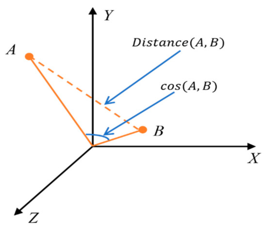
Figure 1.
Cosine similarity.
As a result, the ability to explore is rewarded by avoiding premature convergence in higher-dimensional target spaces.
3.3. A Novel Opposition-Based Learning Restart Mechanism
At the time of evolution, individuals in the population may lack diversity and therefore do not update the results of the algorithm. Therefore, if certain conditions are met, the novel opposition-based learning (OBL) restart mechanism is implemented. The pseudocode is shown in Algorithm 1.
| Algorithm 1: A novel OBL restart mechanism |
| 1: if λ = ξ 2: for do 3: Generate the opposite vector using Equation (27) 4: Calculate the fitness value ; 5: 6: Replace with a fitter one between and 7: end for 8: end if |
In general, the evolutionary algorithm first obtains the feasible solution and then searches for the optimal solution in the solution space according to the fitness of the feasible solution. Various evolutionary algorithms search in different ways, but they all essentially have a random factor. In recent years, opposition-based learning has been widely applied in the evolutionary algorithm [48,49]. The main principle of opposition-based learning (OBL) is to replace random search with symmetric search, which can significantly improve the searching ability of the algorithm [50,51,52,53].
The inventors of OBL argue that given a random number, its opposite is more likely to be near the solution than a random point in the search space. Therefore, by comparing a number with its opposite number, the convergence time for finding the best solution can be reduced. For example, if the current solution X is −1 and the globally optimal value is 2, the X* solution that is symmetric about the origin of the coordinate axis is 1, and X is 3 away from the globally optimal value. However, the global optimal value of X* is only 1. Thus, the solution X* is closer to the global optimal, as shown in Figure 2.
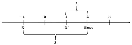
Figure 2.
The opposition-based learning (OBL) principle.
Although the opposition-based learning method improves the searching capability of the algorithm to a great extent, opposition-based learning is too fixed and the tuning effect of the small space is not good. Therefore, in this paper, an innovative way is proposed to improve the original OBL which adds a random weight factor
. For each individual
, a different individual
is randomly selected in the population, where
and
. Then, P is recombined and obtain a new point. Finally, the opposite operation is performed at the merge point. In this way, the resulting position is not a fixed symmetric position, but a random position between the symmetric position and the central position. This is as shown in Equation (27).
Here, is the opposite of , and is the vector of the individual in the population. and are dynamic interval boundaries
and are respectively the minimum and maximum values of the dimension in the current search space. denotes the generation. σ is a random number in the range of .
In order to solve the problem of how to judge the search stagnation, the variable coefficient λ is introduced to determine whether the population has low diversity or whether the algorithm converges to the local optimum. The variable coefficient λ is the variable coefficient of the error of all individual members. The variable coefficient λ is described as follows:
Here, represents the standard deviation of the error value of all individuals and represents to the average value of the error values of all individuals. The restart policy is enacted if the condition in Equation (29) is met.
where ξ is the predetermined parameter used to control the restart.
| Algorithm 2: MjSO |
| 1: Archive ← ∅ 2: Initialize population = (. . . , ) randomly 3: Set all values in to 0.5 4: Set all values in to 0.5 5: //index counter 6: while the termination criteria are not meet do 7: ← ∅, ← ∅ 8: for to do 9: ← select from randomly 10: if = then 11: ← 0.9 12: ← 0.9 13: end if 14: if < 0 then 15: 16: else 17: ← (, 0.1) 18: end if 19: if < 0.25 then 20: ← max ( 0.7) 21: else if < 0.5 then 22: ← max (, 0.6) 23: end if 24: if 25: 26: else 27: ← (, 0.1) 28: if < 0.6 and > 0.7 then 29: ← 0.7 30: end if 31: end if 32: ← current-to-pBest-w/1/bin using Equation (21) 33: end for 34: for i = 1 to do 35: if ≤ then 36: ← 37: else 38: ← 39: end if 40: if ≤ then 41: →, → , → 42: end if 43: Shrink , if necessary 44: Update and 45: Apply LPSR strategy//linear population size reduction 46: Apply Algorithm 1 47: Update using Equation (20) 48: end for 49: 50: end while |
4. The Experimental Setup
Usually, due to the lack of a theoretical proof, it is difficult to evaluate the degree of “good” of an optimized algorithm; therefore, the benchmark function plays an important role in the performance evaluation of these algorithms. Therefore, the performance of the MjSO algorithm proposed in this paper is evaluated using the CEC 2017 actual parameter single objective optimization competition as the benchmark. The benchmark test includes 30 test functions with various characteristics. D is the dimension of the problem, and the problem is tested using ,, , and. Functions 1~3 are unimodal functions, functions 4~10 are multimodal functions, functions 11~20 are mixed functions, and functions 21~30 are composite functions. These unconstrained benchmark functions are shown in Table 1. The termination criteria for the iteration of the algorithm are when the maximum number of fitness function evaluations () and the minimum error value (when the error value is less than , it is considered to have found the optimal value) are and , respectively. The search range [xmin, xmax] = [−100, 100], and 51 independent repeated experiments are conducted for each function. In order to statistically compare the quality of the solutions of different algorithms, two nonparametric statistical hypothesis tests were used to analyze the results: (1) the Friedman test was used to sort all the comparison algorithms [54]; (2) all of the comparison algorithms were evaluated using the Wilcoxon’s signed rank test with a significance level α = 0.05.

Table 1.
Congress on Evolutionary Computation (CEC) 2017 unconstrained benchmark functions.
Each algorithm has its own parametric optimization method to control the influence of parameters on the algorithm. The algorithm LSHADE uses ParamILS [55] which is a versatile and efficient automatic parameter tuner. The parameters in jSO are kept unchanged according to the parameters setting in the LSHADE, except the following parameters: , , , and . The author of algorithm EBLSHADE thinks that it is difficult to determine the optimal values of the control parameters for a variety of problems with different characteristics at different stages of evolution. Therefore, for achieving good performance, the algorithm LSHADE parameter adaptation method was used in EBLSHADE. The algorithm SALSHADE-cnEPSin introduced the method of adaptive parameters by using Weibull distribution-based scaling factor and exponentially decreasing crossover rate. The algorithm ELSHADE-SPACMA performs semi-parameter adaptation (SPA) for F and Cr, and proposes a semi-parameter adaptation strategy to solve parameter setting problem. The parameter settings of each algorithm are consistent with the recommended values of the original papers [31,32,34,56,57], as shown in Table 2.
Table 2.
Parameter settings.
4.1. Experimental Environment
All these experiments were conducted on a PC with an Intel(R) Core (TM) i7-9700 CPU @ 3.0 GHz, 32 GB of RAM and the Windows 10 Professional Edition operating system; and all these algorithms were implemented using Matlab 2017b.
4.2. Clustering Analysis
The clustering algorithm selected in this paper is density-based noisy application spatial clustering (DBSCAN) [58]. It is a clustering algorithm based on the clustering density, which can find clusters with arbitrary shapes. The DBSCAN algorithm needs to set two control parameters and a distance measure. The settings are as follows:
- The core point distance is that Eps = 1% of the decision space. For the CEC2017 benchmark set, Eps = 2.
- The minimum number of clusters MinPts = 4 (minimum number of individuals with mutations).
- The distance measurement is equal to Chebyshev distance [59]. If the distance between any corresponding attributes of two individuals is greater than 1% of the decision space, they are not considered to be directly dense-reachable.
4.3. Population Diversity
The population diversity (PD) measure used in this paper was taken from reference [60] and calculated based on the square root of the sum of individual dimensions, as shown in Equation (31), and the deviation from the corresponding mean, as shown in Equation (30):
where i is the iteration of the individual population, and j is the iteration of the individual dimension.
5. Experimental Results and Analysis
This section presents the experimental results of this paper. Table 3, Table 4, Table 5, Table 6, Table 7 shows the results of the comparison between MjSO and the latest proposed LSHADE variant algorithms (EBLSAHDE, ELSHADE SPACMA, and SALSHADE-cnEPSin) and their original versions (jSO and LSHADE) on , , , and . All the experimental results adopt the error value. According to the experimental results, three symbols () are set to compare the advantages and disadvantages of the algorithm. The symbols () indicate that MjSO performed significantly better (), significantly worse (), or not significantly different better or worse () compared to other compared algorithms using the Wilcoxon rank-sum test (significantly, α = 0.05). For each benchmark function from F1 to F30, the best value among the six algorithms is shown in bold (or bold if the performance is similar).
Table 3.
Algorithm comparison between five powerful differential evolution (DE) variants and our MjSO algorithm on optimization under f1–f30 of our test suite.
Table 4.
Algorithm comparison between five powerful DE variants and our MjSO algorithm on optimization under f1–f30 of our test suite.
Table 5.
Algorithm comparison between five powerful DE variants and our MjSO algorithm on optimization under f1–f30 of our test suite.
Table 6.
Algorithm comparison between five powerful DE variants and our MjSO algorithm on optimization under f1–f30 of our test suite.
Table 7.
Summarized statistical testing (Wilcoxon rank-sum test at the 0.05 significance level).
As shown in Table 3, the six DE variants compared perform equally well on benchmarks f1, f2, f3, f4, f6, and f9 and the global optimal values for these benchmarks were always found within 51 independent runs. In addition, compared with EBLSHADE, the proposed MjSO algorithm achieved better performance for 14 and similar performance for 13 out of 30 benchmarks. Compared with SALSHADE-cnEPSin, our proposed MjSO algorithm achieved better performance 8 times and similar performance 20 times. Compared to jSO, our algorithm achieved better performance 13 times and similar performance 16 times. Compared to LSHADE, our algorithm achieved better performance 16 times and similar performance 13 times. Compared to ELSHADE-SPACMA, our algorithm achieved better performance 13 times and similar performance 17 times. In summary, the proposed MjSO algorithm achieved the best performance in optimization.
It can be seen from Table 4 that the six DE variants compared performed equally well on the benchmarks f1, f2, f3, and f9 and that the global optimal values for these benchmarks were always found within 51 separate runs. The global optimal values of SALSHADE-cnEPSin, ELSHADE-SPACMA and MjSO can be found on f6 each time the algorithms run. In addition, compared with EBLSHADE, the proposed MjSO algorithm achieved better performance in 16 and similar performance in 14 out of 30 benchmarks. Compared with SALSHADE-cnEPSin, our algorithm achieved better performance 19 times and similar performance 10 times. Compared to jSO, our algorithm achieved better performance 20 times and similar performance 10 times. Compared to LSHADE, our algorithm achieved better performance 17 times and similar performance 13 times. Compared to ELSHADE-SPACMA, our algorithm achieved better performance 18 times and similar performance 12 times. From what has been discussed above, the MjSO algorithm achieved the best performance on optimization.
In Table 5, the six DE variants compared performed equally well on the benchmarks f1, f2, f3, and f9 and the global optimal values for these benchmarks were always found within 51 separate runs. In addition, compared with EBLSHADE, the proposed MjSO algorithm achieved better performance in 23 and similar performance in 7 out of 30 benchmarks. Compared with SALSHADE-cnEPSin, our algorithm achieved better performance 26 times and similar performance 4 times. Compared with jSO, our algorithm achieved better performance 20 times and similar performance 10 times. Compared with LSHADE, our algorithm achieved better performance 20 times and similar performance 10 times. Compared with ELSHADE-SPACMA, our algorithm achieved better performance 7 times and similar performance 12 times. In summary, the MjSO algorithm achieved the best performance on optimization.
Table 6 shows the performances of the EBLSHADE, jSO, LSHADE, ELSHADE SPACMA, and MjSO algorithms during each run seeking to find the global optimal value in f1. The global optimal values of SALSHADE-cnEPSin, ELSHADE-SPACMA, and MjSO can be found on f9 every time the algorithms run. In addition, compared with EBLSHADE, the proposed MjSO algorithm achieved better performance in 24 and similar performance in 2 out of 30 benchmarks. Compared with SALSHADE-cnEPSin, our algorithm achieved better performance 25 times and similar performance 1 time. Compared to jSO, our algorithm achieved better performance 24 times and similar performance 2 times. Compared to LSHADE, our algorithm achieved better performance 25 times and similar performance 2 times. Compared to ELSHADE-SPACMA, our algorithm achieved better performance 23 times and similar performance 3 times. In summary, the proposed MjSO algorithm achieved the best performance on optimization. From this, the modified algorithm MjSO proposed by us achieved better results on high-dimensional problems compared with the other five algorithms.
In addition, the effectiveness of the proposed MjSO algorithm with respect to convergence speed was also verified. The convergence diagram is shown in Figure 3, Figure 4, Figure 5, Figure 6, Figure 7, Figure 8, Figure 9, Figure 10. Figure 3 and Figure 4 show the convergence curves of the partial test functions on optimization for the MjSO algorithm and the other five comparison algorithms. Figure 5 and Figure 6 show the convergence curves of the partial test functions on optimization for the MjSO algorithm and the other five comparison algorithms. Figure 7 and Figure 8 show the convergence curves of the partial test functions on optimization for the MjSO algorithm and the other five comparison algorithms. Figure 9 and Figure 10 show the convergence curves of the partial test functions on optimization for the MjSO algorithm and the other five comparison algorithms. In most cases, in the early stage of the optimization process, most MjSO algorithms have similar convergence to the original algorithm, but in the middle stage of the optimization process, the MjSO algorithm maintains a longer search state and achieves a better objective function value in the middle and late stages of the optimization. The convergence rate of the red curve of the proposed MjSO algorithm is usually slow, but it can achieve a better objective function value.
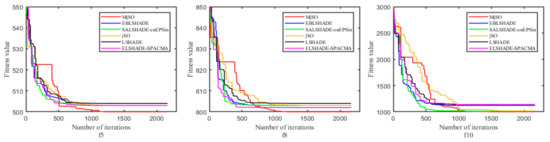
Figure 3.
Convergence speed comparison on optimization.
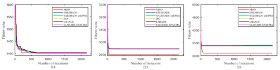
Figure 4.
Convergence speed comparison on optimization.
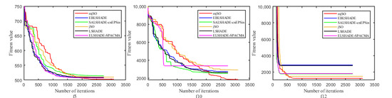
Figure 5.
Convergence speed comparison on optimization.
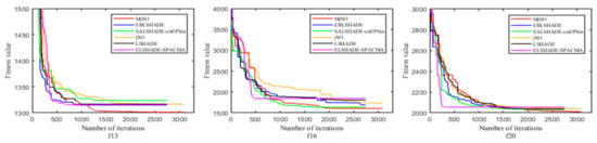
Figure 6.
Convergence speed comparison on optimization.
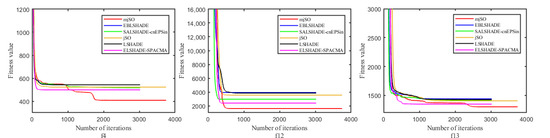
Figure 7.
Convergence speed comparison on optimization.
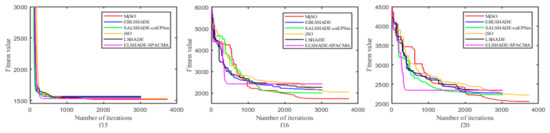
Figure 8.
Convergence speed comparison on optimization.
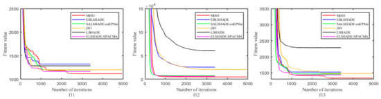
Figure 9.
Convergence speed comparison on optimization.
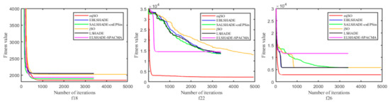
Figure 10.
Convergence speed comparison on optimization.
Table A1, Table A2, Table A3, Table A4 show the number of independent experiments (#runs) of the proposed MjSO algorithm and its original version jSO, the mean number of iterations (mean CO) of the first clustering during the independent experiment running period, and the mean population density (mean PD) of these corresponding iterations.
It can be seen from the table that in most cases, the proposed MjSO algorithm had fewer clustering times (#runs), later clustering (mean CO), and greater population density (mean PD), i.e., better population diversity. In summary, in most cases, MjSO maintained the diversity of the population and prolonged the search stage in the optimization process. This also proves the effectiveness of the modifications we introduced.
According to the Friedman rankings in Table A5, Table A6, Table A7, Table A8, the MjSO algorithm performed the best in all dimensions and was ranked first. Table A9 shows that in all dimensions, the null hypothesis was rejected, which verifies the correctness of the above Friedman rankings. Thus, in the , , , and problems, the MjSO proposed by us is superior to the original jSO and LSHADE algorithms. Compared with more advanced algorithms such as EBLSHADE, SALSHADE-cnEPSin and ELSHADE-SPACMA, it has obvious advantages.
6. MjSO for Engineering Problems
In this section, three constrained engineering problems are employed to demonstrate the performance of MjSO, namely, the pressure vessel design problem, tension/compression spring design problem, and welding beam design problem [61,62]. These engineering problems are inspired by real world cases and there exist some real constrained conditions and one objective functions. Therefore, transforming them into constrained optimization problems is the general method to handle them.
6.1. Pressure Vessel Design Problem
The goal of the pressure vessel design problem is to minimize the total cost of the cylindrical pressure vessel [33]. It has four design variables: shell thickness (), ball thickness (), cylindrical shell radius (), and shell length (). These four optimization variables constitute a four-dimensional constrained optimization problem, which is . Figure 11 shows the pressure vessel and parameters involved in the design. The mathematical model of the pressure vessel design problem can be expressed as follows:
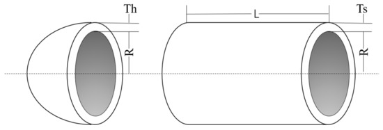
Figure 11.
Pressure vessel design problem.
Minimize
Subject to
where
Table 8 shows the seven test algorithms running independently for 51 times to solve the pressure vessel design problem, the optimal value of the optimization results of each algorithm, and the corresponding optimal solution (the optimal design value of the optimization variable). As can be seen from the table, compared with all other algorithms, MjSO achieved better results in the pressure vessel design problem: the MjSO of the objective function value of 5885.522643154713 obtained the best solution.
Table 8.
Comparison of results for pressure vessel design problem.
6.2. Tension/Compression Spring Design Problem
The goal of this design problem is to minimize the weight of the tension/compression spring shown in Figure 12. The design has three design variables: the wire diameter (d), mean coil diameter (D), and number of active coils (N), which are subject to one linear and three nonlinear inequality constraints on shear stress, surge frequency, and deflection. The mathematical model of tension/compression spring design problem can be expressed as follows:
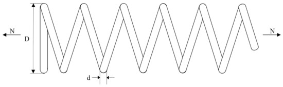
Figure 12.
Compression/tension spring design problem.
Consider
minimize
subject to
where
As can be seen from Table 9, compared with all other algorithms, MjSO achieved better results in the design of tension/compression springs: the MjSO with the objective function value of 0.012665255009 got the best solution.
Table 9.
Comparison of results for compression/tension spring design problem.
6.3. Welded Beam Design Problem
The purpose of the welded beam design problem is to minimize the cost of the welded beam shown in Figure 13. It contains four design variables: the thickness of the weld (h), length of the clamped bar (l), the height of the bar (t), and thickness of the bar (b), which are subject to two linear and five nonlinear inequality constraints on shear stress, bending stress in the beam, buckling load, and end deflection of the beam. The design is expressed as follows:
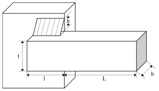
Figure 13.
Welding beam design problem.
Consider
Minimize
Subject to
where
Table 10 presents the best weights and the optimal values for the decision variables from MjSO and several other algorithms. As can be seen from the table, when the four parameters h, l, t, and b are set as 0.2057, 3.4704, 9.0366, and 0.2057, respectively, the minimum manufacturing cost with MjSO is 1.7248. The solution from MjSO is better than the solutions from the other algorithms.
Table 10.
Comparison of results for welded beam design problem.
In this section, the proposed algorithm MjSO was used to solve three kinds of engineering problems and compared with the other six algorithms. There is a phenomenon worthy of analysis and explanation, as can be seen from the results: (1) in the three engineering problems, MjSO achieved the best results, which is significantly better than the DE series basic algorithms (DE, LSHADE). (2) For the latest LSHADE variant algorithm, in pressure vessel design problem, the result of MjSO was close to EBLSHADE; in the tension/compression spring design problem and welded beam design problem, the result of MjSO was not much different from the result of SALSHADE-cnEPSin and EBLSHADE. (3) Through Table 3 and Table 8, Table 9, Table 10, it can be found that the performance of MjSO, EBLSHADE, and SALSHADE-cnEPSin on engineering problems was consistent with the performance on
CEC’17 benchmark functions. This shows the effectiveness of the algorithm. (4) Due to the accuracy of the results generated by the algorithm on the model [40], it can be found that although the numerical results are relatively close, the progress made by MjSO is still significant.
7. Conclusions
This article proposes an improved jSO algorithm (MjSO) for engineering optimization design problems. In our proposed MjSO algorithm, first, a parameter control strategy based on a symmetric search process is applied for the scaling factor to balance exploration and exploitation. In addition, in order to improve the loss of population diversity in the evolutionary process, a parameter adaptive mechanism based on the “cosine similarity” is proposed. And a novel opposition-based learning restart mechanism to the MjSO algorithm to jump out of the local optimum. Through comparative experiments on 30 CEC 2017 benchmark functions, MjSO ranked first in the Friedman test in different dimensions, proving the effectiveness and competitiveness of the proposed algorithm. Finally, through the comparative analysis of the optimization design results of the six comparison algorithms, it is clearly shown that the improved algorithm in this paper has good solution quality and effectiveness in solving engineering optimization design problems.
In future work, we will continue to improve the optimization performance of the algorithm and improve its robustness, apply it to more engineering optimization design problems, and improve its ability to solve problems in engineering practice.
Author Contributions
Conceptualization, H.K.; methodology, H.K.; project administration, Z.L. and Y.S.; software, X.S.; validation, X.S. and Q.C.; visualization, Z.L. and Q.C.; formal analysis, H.K.; investigation, Q.C.; resources, Y.S.; data curation, Z.L.; writing—original draft preparation, Z.L.; writing—review and editing, H.K. and X.S.; supervision, X.S.; funding acquisition, Y.S. All authors have read and agreed to the published version of the manuscript.
Funding
This research was funded by National Natural Science Foundation of China, grant number 61663046, 1876166. This research was funded by Open Foundation of Key Laboratory of Software Engineering of Yunnan Province, grant number 2020SE308, 2020SE309. This research was funded by Science Research Foundation of Yunnan Education Committee of China, grant number 2020Y0004.
Institutional Review Board Statement
Not applicable.
Informed Consent Statement
Not applicable.
Data availability Statement
Data sharing is not applicable to this article.
Conflicts of Interest
The authors declare no conflict of interest.
Appendix A
Table A1.
Clustering and population diversity of jSO and MjSO on the CEC2017 in .
Table A1.
Clustering and population diversity of jSO and MjSO on the CEC2017 in .
| No | jSO | MjSO | ||||
|---|---|---|---|---|---|---|
| #runs | Mean CO | Mean PD | #runs | Mean CO | Mean PD | |
| f1 | 51 | 5.67E+01 | 3.93E+01 | 51 | 4.58E+01 | 3.17E+01 |
| f2 | 51 | 8.84E+01 | 3.06E+01 | 51 | 6.99E+01 | 2.92E+01 |
| f3 | 51 | 8.64E+01 | 7.00E+00 | 51 | 6.97E+01 | 7.19E+00 |
| f4 | 51 | 6.01E+01 | 1.18E+01 | 51 | 4.70E+01 | 1.13E+01 |
| f5 | 48 | 1.19E+03 | 3.28E+01 | 50 | 1.11E+03 | 3.11E+01 |
| f6 | 51 | 9.35E+01 | 8.47E+00 | 51 | 7.21E+01 | 8.84E+00 |
| f7 | 49 | 1.40E+03 | 1.05E+01 | 46 | 1.32E+03 | 1.02E+01 |
| f8 | 50 | 1.19E+03 | 3.40E+01 | 51 | 1.06E+03 | 3.32E+01 |
| f9 | 51 | 9.00E+01 | 7.45E+00 | 51 | 6.95E+01 | 7.80E+00 |
| f10 | 47 | 1.37E+03 | 8.31E+01 | 50 | 1.29E+03 | 7.08E+01 |
| f11 | 51 | 3.90E+02 | 2.13E+01 | 51 | 3.35E+02 | 1.98E+01 |
| f12 | 51 | 2.76E+02 | 4.31E+01 | 51 | 1.86E+02 | 3.40E+01 |
| f13 | 51 | 8.30E+02 | 1.35E+01 | 51 | 6.52E+02 | 1.35E+01 |
| f14 | 51 | 8.12E+02 | 2.75E+01 | 47 | 6.06E+02 | 3.25E+01 |
| f15 | 51 | 3.26E+02 | 1.81E+01 | 51 | 2.62E+02 | 1.80E+01 |
| f16 | 49 | 8.87E+02 | 1.77E+01 | 41 | 5.95E+02 | 2.61E+01 |
| f17 | 1 | 1.89E+03 | 1.47E+01 | 2 | 1.72E+03 | 2.55E+01 |
| f18 | 51 | 3.00E+02 | 2.57E+01 | 51 | 2.40E+02 | 2.40E+01 |
| f19 | 51 | 5.11E+02 | 3.04E+01 | 51 | 3.77E+02 | 2.78E+01 |
| f20 | 47 | 7.52E+02 | 3.69E+01 | 42 | 6.50E+02 | 3.44E+01 |
| f21 | 51 | 5.70E+02 | 4.52E+01 | 51 | 5.78E+02 | 5.50E+01 |
| f22 | 51 | 5.68E+01 | 7.83E+00 | 51 | 4.50E+01 | 1.11E+01 |
| f23 | 51 | 8.08E+02 | 2.96E+01 | 51 | 6.38E+02 | 2.44E+01 |
| f24 | 51 | 8.42E+02 | 2.89E+01 | 51 | 6.77E+02 | 3.64E+01 |
| f25 | 51 | 7.75E+01 | 1.85E+01 | 51 | 6.37E+01 | 2.34E+01 |
| f26 | 51 | 6.12E+01 | 6.77E+00 | 51 | 5.09E+01 | 7.10E+00 |
| f27 | 51 | 1.05E+02 | 1.74E+01 | 51 | 8.44E+01 | 1.98E+01 |
| f28 | 51 | 8.25E+01 | 2.42E+01 | 51 | 6.89E+01 | 2.71E+01 |
| f29 | 24 | 1.59E+03 | 4.41E+01 | 24 | 1.48E+03 | 3.85E+01 |
| f30 | 51 | 1.60E+02 | 1.32E+01 | 51 | 1.24E+02 | 1.31E+01 |
Table A2.
Clustering and population diversity of jSO and MjSO on the CEC2017 in .
Table A2.
Clustering and population diversity of jSO and MjSO on the CEC2017 in .
| No | jSO | MjSO | ||||
|---|---|---|---|---|---|---|
| #runs | Mean CO | Mean PD | #runs | Mean CO | Mean PD | |
| f1 | 51 | 1.07E+02 | 2.37E+01 | 51 | 9.13E+01 | 2.82E+01 |
| f2 | 51 | 2.81E+02 | 1.77E+01 | 51 | 2.21E+02 | 1.77E+01 |
| f3 | 51 | 1.90E+02 | 7.05E+00 | 51 | 1.72E+02 | 6.93E+00 |
| f4 | 51 | 1.40E+02 | 8.45E+00 | 51 | 1.11E+02 | 8.20E+00 |
| f5 | 47 | 2.32E+03 | 4.46E+01 | 48 | 2.34E+03 | 4.15E+01 |
| f6 | 51 | 1.82E+02 | 7.46E+00 | 51 | 1.52E+02 | 7.31E+00 |
| f7 | 34 | 2.49E+03 | 1.47E+01 | 36 | 2.54E+03 | 1.29E+01 |
| f8 | 48 | 2.26E+03 | 5.00E+01 | 42 | 3.34E+03 | 4.45E+01 |
| f9 | 51 | 1.77E+02 | 7.19E+00 | 51 | 1.47E+02 | 7.05E+00 |
| f10 | 17 | 2.76E+03 | 1.42E+02 | 22 | 2.59E+03 | 1.48E+02 |
| f11 | 51 | 1.17E+03 | 2.70E+01 | 51 | 1.22E+03 | 2.87E+01 |
| f12 | 51 | 4.77E+02 | 1.85E+01 | 51 | 5.09E+02 | 2.00E+01 |
| f13 | 51 | 8.72E+02 | 9.56E+00 | 51 | 9.66E+02 | 9.88E+00 |
| f14 | 29 | 2.01E+03 | 2.38E+01 | 26 | 2.88E+03 | 1.80E+01 |
| f15 | 51 | 9.12E+02 | 1.45E+01 | 51 | 1.05E+03 | 1.71E+01 |
| f16 | 30 | 2.86E+03 | 1.61E+01 | 29 | 2.80E+03 | 1.65E+01 |
| f17 | 12 | 2.82E+03 | 5.36E+01 | 7 | 3.74E+03 | 7.99E+01 |
| f18 | 20 | 2.50E+03 | 6.02E+00 | 15 | 3.20E+03 | 8.67E+00 |
| f19 | 51 | 1.41E+03 | 1.46E+01 | 51 | 1.42E+03 | 1.30E+01 |
| f20 | 14 | 2.93E+03 | 3.33E+01 | 8 | 2.85E+03 | 6.11E+01 |
| f21 | 48 | 2.36E+03 | 4.28E+01 | 50 | 2.25E+03 | 4.27E+01 |
| f22 | 51 | 1.15E+02 | 6.68E+00 | 51 | 9.66E+01 | 6.54E+00 |
| f23 | 50 | 2.01E+03 | 4.25E+01 | 51 | 1.86E+03 | 3.62E+01 |
| f24 | 51 | 1.82E+03 | 4.62E+01 | 51 | 1.79E+03 | 3.94E+01 |
| f25 | 51 | 1.27E+02 | 7.39E+00 | 51 | 1.04E+02 | 7.14E+00 |
| f26 | 51 | 1.68E+03 | 3.07E+01 | 51 | 1.15E+03 | 1.80E+01 |
| f27 | 51 | 3.44E+02 | 1.59E+01 | 51 | 2.53E+02 | 2.03E+01 |
| f28 | 51 | 1.58E+02 | 1.15E+01 | 51 | 1.31E+02 | 9.79E+00 |
| f29 | 29 | 2.77E+03 | 5.36E+01 | 24 | 2.72E+03 | 4.26E+01 |
| f30 | 51 | 2.85E+02 | 1.26E+01 | 51 | 2.15E+02 | 1.34E+01 |
Table A3.
Clustering and population diversity of jSO and MjSO on the CEC2017 in .
Table A3.
Clustering and population diversity of jSO and MjSO on the CEC2017 in .
| No | jSO | MjSO | ||||
|---|---|---|---|---|---|---|
| #runs | Mean CO | Mean PD | #runs | Mean CO | Mean PD | |
| f1 | 51 | 1.20E+02 | 9.52E+00 | 51 | 1.32E+02 | 1.74E+01 |
| f2 | 51 | 3.95E+02 | 1.28E+01 | 51 | 3.68E+02 | 1.32E+01 |
| f3 | 51 | 2.43E+02 | 7.88E+00 | 51 | 2.52E+02 | 7.55E+00 |
| f4 | 51 | 1.84E+02 | 9.18E+00 | 51 | 1.70E+02 | 8.41E+00 |
| f5 | 44 | 2.97E+03 | 5.62E+01 | 44 | 2.83E+03 | 5.57E+01 |
| f6 | 51 | 1.95E+02 | 7.93E+00 | 51 | 1.98E+02 | 7.67E+00 |
| f7 | 35 | 2.99E+03 | 1.86E+01 | 34 | 3.03E+03 | 1.77E+01 |
| f8 | 45 | 3.00E+03 | 5.46E+01 | 44 | 2.90E+03 | 5.47E+01 |
| f9 | 51 | 1.90E+02 | 7.75E+00 | 51 | 1.89E+02 | 7.50E+00 |
| f10 | 14 | 3.49E+03 | 1.29E+02 | 17 | 3.43E+03 | 1.54E+02 |
| f11 | 51 | 1.84E+03 | 3.05E+01 | 51 | 1.85E+03 | 2.97E+01 |
| f12 | 51 | 3.67E+02 | 1.08E+01 | 51 | 4.43E+02 | 1.25E+01 |
| f13 | 51 | 7.42E+02 | 1.12E+01 | 51 | 9.27E+02 | 1.15E+01 |
| f14 | 51 | 1.67E+03 | 1.33E+01 | 50 | 1.84E+03 | 1.43E+01 |
| f15 | 51 | 8.34E+02 | 1.20E+01 | 51 | 1.13E+03 | 1.65E+01 |
| f16 | 41 | 3.47E+03 | 8.42E+00 | 37 | 3.41E+03 | 1.12E+01 |
| f17 | 15 | 3.58E+03 | 7.67E+00 | 10 | 3.52E+03 | 2.62E+01 |
| f18 | 51 | 8.67E+02 | 9.25E+00 | 51 | 1.14E+03 | 9.77E+00 |
| f19 | 51 | 1.46E+03 | 1.23E+01 | 51 | 1.63E+03 | 1.37E+01 |
| f20 | 24 | 3.43E+03 | 2.04E+01 | 20 | 4.44E+03 | 2.19E+01 |
| f21 | 47 | 2.94E+03 | 5.73E+01 | 43 | 2.93E+03 | 5.60E+01 |
| f22 | 37 | 1.64E+03 | 3.82E+01 | 36 | 9.58E+02 | 3.10E+01 |
| f23 | 48 | 2.69E+03 | 5.35E+01 | 47 | 2.64E+03 | 4.69E+01 |
| f24 | 51 | 2.59E+03 | 4.76E+01 | 50 | 2.12E+03 | 3.38E+01 |
| f25 | 51 | 1.94E+02 | 8.44E+00 | 51 | 1.69E+02 | 7.77E+00 |
| f26 | 51 | 2.36E+03 | 3.69E+01 | 51 | 1.40E+03 | 1.43E+01 |
| f27 | 51 | 3.00E+02 | 1.05E+01 | 51 | 2.15E+02 | 8.77E+00 |
| f28 | 51 | 1.71E+02 | 9.04E+00 | 51 | 2.54E+02 | 1.03E+01 |
| f29 | 32 | 3.34E+03 | 5.63E+01 | 23 | 3.34E+03 | 5.09E+01 |
| f30 | 51 | 3.28E+02 | 1.11E+01 | 51 | 4.22E+02 | 3.08E+01 |
Table A4.
Clustering and population diversity of jSO and MjSO on the CEC2017 in .
Table A4.
Clustering and population diversity of jSO and MjSO on the CEC2017 in .
| No | jSO | MjSO | ||||
|---|---|---|---|---|---|---|
| #runs | Mean CO | Mean PD | #runs | Mean CO | Mean PD | |
| f1 | 51 | 1.37E+02 | 9.05E+00 | 51 | 1.94E+02 | 1.15E+01 |
| f2 | 51 | 5.10E+02 | 1.09E+01 | 51 | 5.80E+02 | 1.04E+01 |
| f3 | 51 | 3.75E+02 | 9.86E+00 | 51 | 4.08E+02 | 9.16E+00 |
| f4 | 51 | 2.01E+02 | 9.29E+00 | 51 | 2.32E+02 | 9.04E+00 |
| f5 | 50 | 3.93E+03 | 7.09E+01 | 49 | 4.03E+03 | 5.59E+01 |
| f6 | 51 | 2.06E+02 | 9.48E+00 | 51 | 2.79E+02 | 8.85E+00 |
| f7 | 46 | 4.12E+03 | 2.19E+01 | 43 | 4.02E+03 | 2.07E+01 |
| f8 | 45 | 4.04E+03 | 6.76E+01 | 51 | 3.90E+03 | 6.33E+01 |
| f9 | 51 | 2.00E+02 | 9.04E+00 | 51 | 2.62E+02 | 8.70E+00 |
| f10 | 13 | 4.46E+03 | 3.06E+02 | 13 | 4.52E+03 | 2.13E+02 |
| f11 | 51 | 5.27E+02 | 9.79E+00 | 51 | 1.17E+03 | 1.14E+01 |
| f12 | 51 | 3.30E+02 | 1.02E+01 | 51 | 4.53E+02 | 9.08E+00 |
| f13 | 51 | 7.08E+02 | 1.34E+01 | 51 | 9.23E+02 | 1.39E+01 |
| f14 | 51 | 1.01E+03 | 1.02E+01 | 51 | 1.28E+03 | 1.30E+01 |
| f15 | 51 | 4.84E+02 | 1.03E+01 | 51 | 9.30E+02 | 9.53E+00 |
| f16 | 49 | 4.43E+03 | 1.16E+01 | 47 | 4.60E+03 | 9.92E+00 |
| f17 | 33 | 4.66E+03 | 2.45E+01 | 49 | 4.04E+03 | 7.65E+01 |
| f18 | 51 | 5.82E+02 | 9.80E+00 | 51 | 5.88E+02 | 1.40E+01 |
| f19 | 51 | 6.38E+02 | 1.07E+01 | 51 | 1.48E+03 | 1.20E+01 |
| f20 | 26 | 4.64E+03 | 1.16E+01 | 26 | 4.54E+03 | 7.67E+01 |
| f21 | 49 | 3.87E+03 | 6.44E+01 | 51 | 2.41E+02 | 9.42E+00 |
| f22 | 14 | 4.39E+03 | 2.67E+01 | 49 | 3.95E+03 | 6.22E+01 |
| f23 | 50 | 1.72E+03 | 2.38E+01 | 51 | 7.70E+02 | 9.25E+00 |
| f24 | 51 | 1.01E+03 | 1.18E+01 | 51 | 2.12E+02 | 8.49E+00 |
| f25 | 51 | 2.11E+02 | 9.56E+00 | 51 | 2.53E+02 | 9.72E+00 |
| f26 | 51 | 7.98E+02 | 9.50E+00 | 51 | 2.68E+02 | 8.62E+00 |
| f27 | 51 | 3.31E+02 | 9.28E+00 | 51 | 2.93E+02 | 8.93E+00 |
| f28 | 51 | 2.23E+02 | 9.42E+00 | 51 | 2.31E+02 | 8.99E+00 |
| f29 | 51 | 4.38E+03 | 4.21E+01 | 51 | 4.13E+03 | 4.22E+01 |
| f30 | 51 | 5.09E+02 | 1.08E+01 | 51 | 4.55E+02 | 1.01E+01 |
Table A5.
The Friedman ranks of comparative algorithms on CEC2017 in .
Table A5.
The Friedman ranks of comparative algorithms on CEC2017 in .
| Rank | Name | F-Rank |
|---|---|---|
| 0 | MjSO | 2.62 |
| 1 | jSO | 3.43 |
| 2 | SALSHADE-cnEPSin | 3.55 |
| 3 | EBLSHADE | 3.6 |
| 4 | ELSHADE-SPACMA | 3.82 |
| 5 | LSHADE | 3.98 |
Table A6.
The Friedman ranks of comparative algorithms on CEC2017 in .
Table A6.
The Friedman ranks of comparative algorithms on CEC2017 in .
| Rank | Name | F-Rank |
|---|---|---|
| 0 | MjSO | 2.1 |
| 1 | jSO | 3.4 |
| 2 | EBLSHADE | 3.43 |
| 3 | SALSHADE-cnEPSin | 3.95 |
| 4 | LSHADE | 4.05 |
| 5 | ELSHADE-SPACMA | 4.07 |
Table A7.
The Friedman ranks of comparative algorithms on CEC2017 in .
Table A7.
The Friedman ranks of comparative algorithms on CEC2017 in .
| Rank | Name | F-Rank |
|---|---|---|
| 0 | MjSO | 1.9 |
| 1 | ELSHADE-SPACMA | 3.27 |
| 2 | jSO | 3.4 |
| 3 | SALSHADE-cnEPSin | 4.05 |
| 4 | LSHADE | 4.15 |
| 5 | EBLSHADE | 4.23 |
Table A8.
The Friedman ranks of comparative algorithms on CEC2017 in .
Table A8.
The Friedman ranks of comparative algorithms on CEC2017 in .
| Rank | Name | F-Rank |
|---|---|---|
| 0 | MjSO | 1.87 |
| 1 | ELSHADE-SPACMA | 3.35 |
| 2 | SALSHADE-cnEPSin | 3.4 |
| 3 | jSO | 3.78 |
| 4 | EBLSHADE | 3.93 |
| 5 | LSHADE | 4.67 |
Table A9.
Related statistical values obtained of Friedman test for α = 0.05.
Table A9.
Related statistical values obtained of Friedman test for α = 0.05.
| D | Chi-sq’ | Prob > Chi-sq’(p) | Critical Value |
|---|---|---|---|
| 10 | 13.73819163 | 1.74E-02 | 11.07 |
| 30 | 31.07891492 | 9.04E-06 | 11.07 |
| 50 | 38.65745856 | 2.78E-07 | 11.07 |
| 100 | 38.16356513 | 3.50E-07 | 11.07 |
References
- Dhiman, G.; Kumar, V. Multi-objective spotted hyena optimizer: A multi-objective optimization algorithm for engineering problems. Knowl. Based Syst. 2018, 150, 175–197. [Google Scholar] [CrossRef]
- Spall, J. Introduction to Stochastic Search and Optimization; Wiley Interscience: New York, NY, USA, 2003. [Google Scholar]
- Parejo, J.A.; Ruiz-Cortés, A.; Lozano, S.; Fernandez, P. Metaheuristic optimization frameworks: A survey and benchmarking. Soft Comput. 2012, 16, 527–561. [Google Scholar] [CrossRef]
- Zhou, A.; Qu, B.-Y.; Li, H.; Zhao, S.-Z.; Suganthan, P.N.; Zhang, Q. Multiobjective evolutionary algorithms: A survey of the state of the art. Swarm Evol. Comput. 2011, 1, 32–49. [Google Scholar] [CrossRef]
- Droste, S.; Jansen, T.; Wegener, I. Upper and lower bounds for randomized search heuristics in black-box optimization. Theory Comput. Syst. 2006, 39, 525–544. [Google Scholar] [CrossRef]
- Hoos, H.H.; Stützle, T. Stochastic Local Search: Foundations and Applications; Elsevier: Amsterdam, The Netherlands, 2004. [Google Scholar]
- Holland, J. Adaptation in Natural and Artificial Systems: An Introductory Analysis with Application to Biology; Control and artificial intelligence, University of Michigan Press: Ann Arbor, MI, USA, 1975; pp. 106–111. [Google Scholar]
- Kennedy, J.; Eberhart, R. Particle swarm optimization. In Proceedings of the ICNN’95-International Conference on Neural Networks, Perth, WA, Australia, 27 November–1 December 1995; IEEE; pp. 1942–1948. [Google Scholar]
- Storn, R.; Price, K. Differential evolution—A simple and efficient heuristic for global optimization over continuous spaces. J. Glob. Optim. 1997, 11, 341–359. [Google Scholar] [CrossRef]
- Wienholt, W. Minimizing the system error in feedforward neural networks with evolution strategy. In Proceedings of the International Conference on Artificial Neural Networks, Amsterdam, The Netherlands, 13–16 September 1993; Springer: London, UK, 1993; pp. 490–493. [Google Scholar]
- Eltaeib, T.; Mahmood, A. Differential evolution: A survey and analysis. Appl. Sci. 2018, 8, 1945. [Google Scholar] [CrossRef]
- Arafa, M.; Sallam, E.A.; Fahmy, M. An enhanced differential evolution optimization algorithm. In Proceedings of the 2014 Fourth International Conference on Digital Information and Communication Technology and Its Applications (DICTAP), Bangkok, Thailand, 6–8 May 2014; pp. 216–225. [Google Scholar]
- Liu, X.-F.; Zhan, Z.-H.; Zhang, J. Dichotomy guided based parameter adaptation for differential evolution. In Proceedings of the 2015 Annual Conference on Genetic and Evolutionary Computation, Madrid, Spain, 11–15 July 2015; pp. 289–296. [Google Scholar]
- Sallam, K.M.; Sarker, R.A.; Essam, D.L.; Elsayed, S.M. Neurodynamic differential evolution algorithm and solving CEC2015 competition problems. In Proceedings of the 2015 IEEE Congress on Evolutionary Computation (CEC), Sendai, Japan, 25–28 May 2015; pp. 1033–1040. [Google Scholar]
- Viktorin, A.; Pluhacek, M.; Senkerik, R. Network based linear population size reduction in SHADE. In Proceedings of the 2016 International Conference on Intelligent Networking and Collaborative Systems (INCoS), Ostrawva, Czech Republic, 7–9 September 2016; pp. 86–93. [Google Scholar]
- Bujok, P.; Tvrdík, J.; Poláková, R. Evaluating the performance of shade with competing strategies on CEC 2014 single-parameter test suite. In Proceedings of the 2016 IEEE Congress on Evolutionary Computation (CEC), Vancouver, BC, Canada, 24–29 July 2016; pp. 5002–5009. [Google Scholar]
- Viktorin, A.; Pluhacek, M.; Senkerik, R. Success-history based adaptive differential evolution algorithm with multi-chaotic framework for parent selection performance on CEC2014 benchmark set. In Proceedings of the 2016 IEEE Congress on Evolutionary Computation (CEC), Vancouver, BC, Canada, 24–29 July 2016; pp. 4797–4803. [Google Scholar]
- Poláková, R.; Tvrdík, J.; Bujok, P. L-SHADE with competing strategies applied to CEC2015 learning-based test suite. In Proceedings of the 2016 IEEE Congress on Evolutionary Computation (CEC), Vancouver, BC, Canada, 24–29 July 2016; pp. 4790–4796. [Google Scholar]
- Poláková, R.; Tvrdík, J.; Bujok, P. Evaluating the performance of L-SHADE with competing strategies on CEC2014 single parameter-operator test suite. In Proceedings of the 2016 IEEE Congress on Evolutionary Computation (CEC), Vancouver, BC, Canada, 24–29 July 2016; pp. 1181–1187. [Google Scholar]
- Liu, Z.-G.; Ji, X.-H.; Yang, Y. Hierarchical differential evolution algorithm combined with multi-cross operation. Expert Syst. Appl. 2019, 130, 276–292. [Google Scholar] [CrossRef]
- Bujok, P.; Tvrdík, J. Adaptive differential evolution: SHADE with competing crossover strategies. In Proceedings of the International Conference on Artificial Intelligence and Soft Computing, Zakopane, Poland, 14–18 June 2015; pp. 329–339. [Google Scholar]
- Viktorin, A.; Senkerik, R.; Pluhacek, M.; Kadavy, T.; Zamuda, A. Distance based parameter adaptation for differential evolution. In Proceedings of the 2017 IEEE Symposium Series on Computational Intelligence (SSCI), Honolulu, HI, USA, 27 November–1 December 2017; pp. 1–7. [Google Scholar]
- Viktorin, A.; Senkerik, R.; Pluhacek, M.; Kadavy, T. Distance vs. Improvement Based Parameter Adaptation in SHADE. In Proceedings of the Computer Science On-Line Conference, Vsetin, Czech Republic, 25–28 April 2018; 2018; pp. 455–464. [Google Scholar]
- Molina, D.; Herrera, F. Applying Memetic algorithm with Improved L-SHADE and Local Search Pool for the 100-digit challenge on Single Objective Numerical Optimization. In Proceedings of the 2019 IEEE Congress on Evolutionary Computation (CEC), Wellington, New Zealand, 10–13 June 2019; pp. 7–13. [Google Scholar]
- Awad, N.H.; Ali, M.Z.; Suganthan, P.N. Ensemble sinusoidal differential covariance matrix adaptation with Euclidean neighborhood for solving CEC2017 benchmark problems. In Proceedings of the 2017 IEEE Congress on Evolutionary Computation (CEC), San Sebastian, Spain, 5–8 June 2017; pp. 372–379. [Google Scholar]
- Zhao, F.; He, X.; Yang, G.; Ma, W.; Zhang, C.; Song, H. A hybrid iterated local search algorithm with adaptive perturbation mechanism by success-history based parameter adaptation for differential evolution (SHADE). Eng. Optim. 2019. [Google Scholar] [CrossRef]
- Das, S.; Mullick, S.S.; Suganthan, P.N. Recent advances in differential evolution—An updated survey. Swarm Evol. Comput. 2016, 27, 1–30. [Google Scholar] [CrossRef]
- Hansen, N. The CMA evolution strategy: A comparing review. In Towards a New Evolutionary Computation; Springer: Berlin/Heidelberg, Germany, 2006; pp. 75–102. [Google Scholar]
- Das, S.; Suganthan, P.N. Differential evolution: A survey of the state-of-the-art. IEEE Trans. Evol. Comput. 2010, 15, 4–31. [Google Scholar] [CrossRef]
- Al-Dabbagh, R.D.; Neri, F.; Idris, N.; Baba, M.S. Algorithmic design issues in adaptive differential evolution schemes: Review and taxonomy. Swarm Evol. Comput. 2018, 43, 284–311. [Google Scholar] [CrossRef]
- Tanabe, R.; Fukunaga, A.S. Improving the search performance of SHADE using linear population size reduction. In Proceedings of the 2014 IEEE Congress on Evolutionary Computation (CEC), Beijing, China, 6–11 July 2014; pp. 1658–1665. [Google Scholar]
- Brest, J.; Maučec, M.S.; Bošković, B. Single objective real-parameter optimization: Algorithm jSO. In Proceedings of the 2017 IEEE Congress on Evolutionary Computation (CEC), San Sebastian, Spain, 5–8 June 2017; pp. 1311–1318. [Google Scholar]
- Mohamed, A.W.; Hadi, A.A.; Fattouh, A.M.; Jambi, K.M. LSHADE with semi-parameter adaptation hybrid with CMA-ES for solving CEC 2017 benchmark problems. In Proceedings of the 2017 IEEE Congress on Evolutionary Computation (CEC), San Sebastian, Spain, 5–8 June 2017; pp. 145–152. [Google Scholar]
- Hadi, A.A.; Wagdy, A.; Jambi, K. Single-Objective Real-Parameter Optimization: Enhanced LSHADE-SPACMA Algorithm; King Abdulaziz Univ.: Jeddah, Saudi Arabia, 2018. [Google Scholar]
- Salgotra, R.; Singh, U.; Singh, G. Improving the adaptive properties of lshade algorithm for global optimization. In Proceedings of the 2019 International Conference on Automation, Computational and Technology Management (ICACTM), London, UK, 24–26 April 2019; pp. 400–407. [Google Scholar]
- Yang, M.; Li, C.; Cai, Z.; Guan, J. Differential evolution with auto-enhanced population diversity. IEEE Trans. Cybern. 2014, 45, 302–315. [Google Scholar] [CrossRef] [PubMed]
- Hongtan, C.; Zhaoguang, L. Improved Differential Evolution with Parameter Adaption Based on Population Diversity. In Proceedings of the 2018 IEEE 3rd International Conference on Image, Vision and Computing (ICIVC), Chongqing, China, 27–29 June 2018; pp. 901–905. [Google Scholar]
- Wang, J.-Z.; Sun, T.-Y. Control the Diversity of Population with Mutation Strategy and Fuzzy Inference System for Differential Evolution Algorithm. Int. J. Fuzzy Syst. 2020, 22, 1979–1992. [Google Scholar] [CrossRef]
- He, X.; Zhou, Y. Enhancing the performance of differential evolution with covariance matrix self-adaptation. Appl. Soft Comput. 2018, 64, 227–243. [Google Scholar] [CrossRef]
- Awad, N.H.; Ali, M.Z.; Mallipeddi, R.; Suganthan, P.N. An improved differential evolution algorithm using efficient adapted surrogate model for numerical optimization. Inf. Sci. 2018, 451, 326–347. [Google Scholar] [CrossRef]
- Subhashini, K.; Chinta, P. An augmented animal migration optimization algorithm using worst solution elimination approach in the backdrop of differential evolution. Evol. Intell. 2019, 12, 273–303. [Google Scholar] [CrossRef]
- Awad, N.; Ali, M.; Liang, J.; Qu, B.; Suganthan, P.; Definitions, P. Evaluation Criteria for the CEC 2017 Special Session and Competition on Single Objective Real-Parameter Numerical Optimization. In Proceedings of the 2017 IEEE Congress on Evolutionary Computation (CEC), San Sebastian, Spain, 5–8 June 2017. [Google Scholar]
- Zhang, J.; Sanderson, A.C. JADE: Adaptive differential evolution with optional external archive. IEEE Trans. Evol. Comput. 2009, 13, 945–958. [Google Scholar] [CrossRef]
- Brest, J.; Maučec, M.S.; Bošković, B. iL-SHADE: Improved L-SHADE algorithm for single objective real-parameter optimization. In Proceedings of the 2016 IEEE Congress on Evolutionary Computation (CEC), Vancouver, Canada, 24–29 July 2016; pp. 1188–1195. [Google Scholar]
- Fan, Q.; Yan, X. Self-adaptive differential evolution algorithm with zoning evolution of control parameters and adaptive mutation strategies. IEEE Trans. Cybern. 2015, 46, 219–232. [Google Scholar] [CrossRef]
- Wang, D.; Lu, H.; Bo, C. Visual tracking via weighted local cosine similarity. IEEE Trans. Cybern. 2014, 45, 1838–1850. [Google Scholar] [CrossRef]
- Van Dongen, S.; Enright, A.J. Metric distances derived from cosine similarity and Pearson and Spearman correlations. arXiv 2012, arXiv:1208.3145. [Google Scholar]
- Luo, J.; He, F.; Yong, J. An efficient and robust bat algorithm with fusion of opposition-based learning and whale optimization algorithm. Intell. Data Anal. 2020, 24, 581–606. [Google Scholar] [CrossRef]
- Shekhawat, S.; Saxena, A. Development and applications of an intelligent crow search algorithm based on opposition based learning. ISA Trans. 2020, 99, 210–230. [Google Scholar] [CrossRef] [PubMed]
- Ergezer, M.; Simon, D. Mathematical and experimental analyses of oppositional algorithms. IEEE Trans. Cybern. 2014, 44, 2178–2189. [Google Scholar] [CrossRef] [PubMed]
- Tizhoosh, H.R. Opposition-based reinforcement learning. J. Adv. Comput. Intell. Intell. Inform. 2006, 10. [Google Scholar] [CrossRef]
- Rahnamayan, S.; Tizhoosh, H.R.; Salama, M.M. Opposition-based differential evolution. EEE Trans. Evol. Comput. 2008, 12, 64–79. [Google Scholar] [CrossRef]
- Rahnamayan, S.; Tizhoosh, H.R.; Salama, M.M. Quasi-oppositional differential evolution. In Proceedings of the 2007 IEEE Congress on Evolutionary Computation, San Sebastian, Spain, 5–8 June 2017; pp. 2229–2236. [Google Scholar]
- Demšar, J. Statistical comparisons of classifiers over multiple data sets. J. Mach. Learn. Res. 2006, 7, 1–30. [Google Scholar]
- Hutter, F.; Hoos, H.H.; Leyton-Brown, K.; Stützle, T. ParamILS: An automatic algorithm configuration framework. J. Artif. Intell. Res. 2009, 36, 267–306. [Google Scholar] [CrossRef]
- Mohamed, A.W.; Hadi, A.A.; Jambi, K.M. Novel mutation strategy for enhancing SHADE and LSHADE algorithms for global numerical optimization. Swarm Evol. Comput. 2019, 50, 100455. [Google Scholar] [CrossRef]
- Salgotra, R.; Singh, U.; Saha, S.; Nagar, A. New improved salshade-cnepsin algorithm with adaptive parameters. In Proceedings of the 2019 IEEE Congress on Evolutionary Computation (CEC), Wellington, New Zealand, 10–13 June 2019; pp. 3150–3156. [Google Scholar]
- Ester, M.; Kriegel, H.-P.; Sander, J.; Xu, X. A density-based algorithm for discovering clusters in large spatial databases with noise. In Proceedings of the Kdd, Menlo Park, CA, USA, August 1996; pp. 226–231. [Google Scholar]
- Deza, M.M.; Deza, E. Encyclopedia of distances. In Encyclopedia of Distances; Springer: Berlin/Heidelberg, Germany, 2009; pp. 1–583. [Google Scholar]
- Poláková, R.; Tvrdík, J.; Bujok, P.; Matoušek, R. Population-size adaptation through diversity-control mechanism for differential evolution. In Proceedings of the MENDEL, 22th International Conference on Soft Computing, Brno, Czech Republic, 8–10 June 2016; pp. 49–56. [Google Scholar]
- Varaee, H.; Ghasemi, M.R. Engineering optimization based on ideal gas molecular movement algorithm. Eng. Comput. 2017, 33, 71–93. [Google Scholar] [CrossRef]
- Askarzadeh, A. A novel metaheuristic method for solving constrained engineering optimization problems: Crow search algorithm. Comput. Struct. 2016, 169, 1–12. [Google Scholar] [CrossRef]


Publisher’s Note: MDPI stays neutral with regard to jurisdictional claims in published maps and institutional affiliations. |
© 2020 by the authors. Licensee MDPI, Basel, Switzerland. This article is an open access article distributed under the terms and conditions of the Creative Commons Attribution (CC BY) license (http://creativecommons.org/licenses/by/4.0/).