1. Introduction
A category theory may be viewed as the newest approach to formalization of mathematical structures by means of a general algebra-based conceptualization. Simultaneously, an exhaustive characterization of category theory encounters different difficulties of a methodological nature. It forms the aftermath of a dichotomy between a purely theoretic provenience of category theory (with its conceptual sources located in homology and universal algebra) and a programming-oriented application area outside its theoretic parent environment. Last, but not least–some vulnerability of the theory to be exploited in the role of a new paradigm in foundations of formal sciences should be also taken into account by such a characterization attempt. One can venture to formulate the thesis that the category theory–initially developed by S. Eilenberg and S. McLane in [
1]–has its Renaissance. It finds its reflection in several different monographs, such as [
2,
3,
4,
5], which elucidate different aspects of the theory and its application area.
The non-static style of thinking in category theory (by contrast to classical set theory) manifests itself in different ways. The main reasoning line in this theory is determined by the sequence of mappings of a gradually increasing degree of abstraction. Morphisms (or simply arrows)–as the most internal mappings–live inside categories and operate between categorial objects. The so-called functors have a more external nature–as they map one category into another category. Finally, the so-called natural transformations operate between functors themselves, thus they form some unique mappings between mappings. Having defined the natural transformations–one can venture to predict their general form.
The main formal tool–often adopted to this task –is the so-called Yoneda’s lemma. It enables predicting a general form of the natural transformations in a relatively smart way and it often simplifies the whole reasoning. There exist many examples, which confirm the thesis. In fact, for monoids and grupoids (broader: for algebraic structures of a cyclic nature They may be generated by a single element.) the form of the natural transformation is predictable from a single value of the so-called
representable functor (introduced in detail in
Section 2) for an initial object of these structures.
1.1. The Paper Motivation
The second distinctive feature of reasoning in category theory is a condition of diagram commutativity. In fact, a majority of important features of different categorial entities (products, co-products, limits, functors, etc.) All of these fundamental concepts may be found in each handbook of category theory, for example, see: [
1,
5]. is just ensured by commutativity of the appropriate diagrams. This property is fundamental for other properties of categorial objects–as categorial entities often form the structures of the appropriate type (products, co-products, categories themselves, etc.) provided that a kind of a commutativity condition (for the appropriate diagrams) holds (see, for example [
1,
5]). Otherwise, the same categorial entities cannot be considered as the structure of this type. Thus, the classical commutativity condition determines a two-valued spectrum of possibilities, which shows that it forms a two-valued logic-based property. It seems that the two-valued logic-based commutativity condition constitutes a universally convenient foundation of categorial reasoning.
Meanwhile, some circumstances seem to decline to the two-valued comprehension of commutativity. At first, many logical concepts, mental mechanisms, and life contexts–potentially suitable to be modeled by objects of category theory–often show their fuzzy nature (see: [
6,
7,
8]). Secondly, many classical mathematical objects–such as groups, graphs or even C
-algebras–found their fuzzy counterparts: fuzzy groups (see: [
9]), fuzzy graphs (see: [
10]), C*-algebras (see: [
11]) in the conceptual framework of the so-called fuzzy mathematics. Meanwhile, it seems that there exists a gap between a potential capability of category theory to be addressed to fuzziness and a current condition of the theory. Thus, the methodological program to refer category theory to different entities of a fuzzy type (both of a mathematical and non-mathematical nature)–generates a need to equip this theory by the appropriate conceptual (and partially formal) tissue–in order to better extract and elucidate different faces of fuzziness.
Unfortunately, many seminal and already classical papers–collected in [
12], such as [
13,
14]—do not propose rather any remedy for this difficulty. In fact, the papers present more a classically (non-fuzzy) categorial depiction of fuzziness in different fields of mathematics, than elaborate a frame of fuzzy category theory itself. Fortunately, was partially performed in a couple of newer papers, such as [
15,
16,
17]. This trend has found its reflection in [
18,
19]. (This paper extends its ideas.)
Meanwhile, the program to fuzzify category theory may be materialized in two ways: either by fuzzifying the categorial entities or by fuzzifying the principles defining them. One can argue that the first idea (reflected by introducing different fuzzy variants of the most important concepts of category theory It refers to fuzzy categories, fuzzy products, fuzzy co-products, etc.) forms too radical decision. In fact, the so-far fuzzification may essentially change the whole scenario of categorial entities and relations between them. The alternative idea (of fuzzifying the principles and properties only) is more accurate–as it enables us to preserve a majority of the classical results and properties of categorial structures and mapping in category theory. Meanwhile, a natural transformation plays a distinguished role among the categorial entities–representing the whole dynamism of categorial reasoning. In [
20] a fuzzy natural transformation was proposed and a fuzzy Yoneda’s lemma was formulated and shown. Unfortunately, this approach only refers to single diagrams, which define their corresponding natural transformations.
The distinguished role of natural transformations and the arsing need to develop a fuzzy category via fuzzifying principles and properties of categorial entities generate a couple of natural questions:
1.2. Paper Objectives and Organization
In accordance with the open questions—formulated in this conceptual scenario, this paper is aimed at:
extending an idea of fuzzy natural transformations towards multi-fuzzy natural transformations–as determined by the multi-fuzzy commutativity condition,
introducing and proving the appropriate version of multi-fuzzy Yoneda’s lemma and
introducing a sketch of the conceptual tissue’ application area concerning the combinatorial problem of error detection (exploiting the so-called Hamming’s distances).
The rest part of the paper is structured as follows.
Section 2 puts forward a terminological framework of further analysis.
Section 3 forms an introduction to the main body of the paper, and it introduces a variety of the multi-fuzzy natural transformations.
Section 4 presents the multi-fuzzy natural transformations’ operational face by its reference to the so-called Hamming’s distances. A multi-fuzzy Yoneda’s lemma is formulated in
Section 5 giving a sketch of its proof.
Section 6 contains a solution of the leading practical problem of the paper.
Section 7 describes state of the art.
Section 8 contains closing remarks.
2. The Conceptual Framework and the Leading Problem Formulation
In this part, the conceptual framework of the analysis is put forward, and the leading problem is formulated The reader may found all the definitions in each book devoted to category theory, for example, in [
4,
6].
2.1. Terminological Background
The notion of the category stems from the algebraic concept of the group of transformation. The term ’transformation’ itself is exploited in this context here as synonymous with the concept of mapping.
Definition 1 (
Group of transformations)
. Let X be an arbitrarily given set, –a set of autotransformations in X. Then the pair , where is a group domain and forms the group operation, is a group of transformations, if these three conditions are satisfied:
If , then (i.e., G is closed on •),
There is a unique element in G to be called the neutral one (it is the identity transformation ),
For each transformation α, there is its inverse transformation (i.e., each transformation is reversible).
A slight generalization of the situation–by rejecting the condition 3 and by admitting the transformations between X and Y (where )–enables us to obtain the following definition of a category (of transformation).
Definition 2 (
Category of transformations)
. Let be some arbitrary sets, form a set of transformations from X to Y. Then the pair is a category of transformations, if it has the following three properties:
If , then (i.e., is closed on •),
There is a unique neutral element in K (the so-called identity transformation ),
For each , it holds (the associativity principle holds for •).
Let us assume that
forms a category. Then the transformations of the category are usually
morphisms or
arrows, but sets
are said to be
objects (of this category). Therefore, each category forms a pair:
where
M forms a set of morphisms (in
K) and
O–a set of objects.
Example 1. A couple of typical examples of categories—their objects and the associated arrows—are collected in the table.| Categories | Objects | Morphisms |
| RelA | sets | binary relations |
| Pos | posets | monotone functions |
| Grp/Gr | groups | morphisms |
| Ring | rings | ring homomorphisms |
| Field | fields | monomorphisms |
| Mon | monoids | monoid homomorphisms |
| Metr | metric spaces | contractions |
| Top | topological spaces | continuous maps |
Definition 3 (
Small and big category)
. A category is small if the collection of its morphisms constitutes a set. Otherwise, if this collection constitutes a proper class, then the category is a big category.
Example 2. The following categories: Set, Gr, Metr, Top are big. Obviously, the category with a singleton consisting of an object o with an identity morphism forms a small category.
Definition 4. Let us assume that and are two categories. A mapping forms a covariant functor if and only if it
- (a)
associates an element to each element and
- (b)
associates to each morphism from a new morphism from such that the following holds:
, for each object X of K,
, for every morphisms: .
Example 3. The so-called power set functor is defined such that it maps each set to its power set, but each function is mapped to the function sending to the image .
Definition 5. A functor is a contravariant functor, if it reverses the direction of morphisms (arrows) in category L (with respect to K).
Example 4. The same scenario as in the previous example, but the powers set functor P sends each morphism to the map sending to the preimage .
In other words, each covariant functor preserves not only the structure of the initial category, but also–the same directions of arrows. By contrast, each contravariant functor preserves the structure of the category itself, but it changes the directions of arrows.
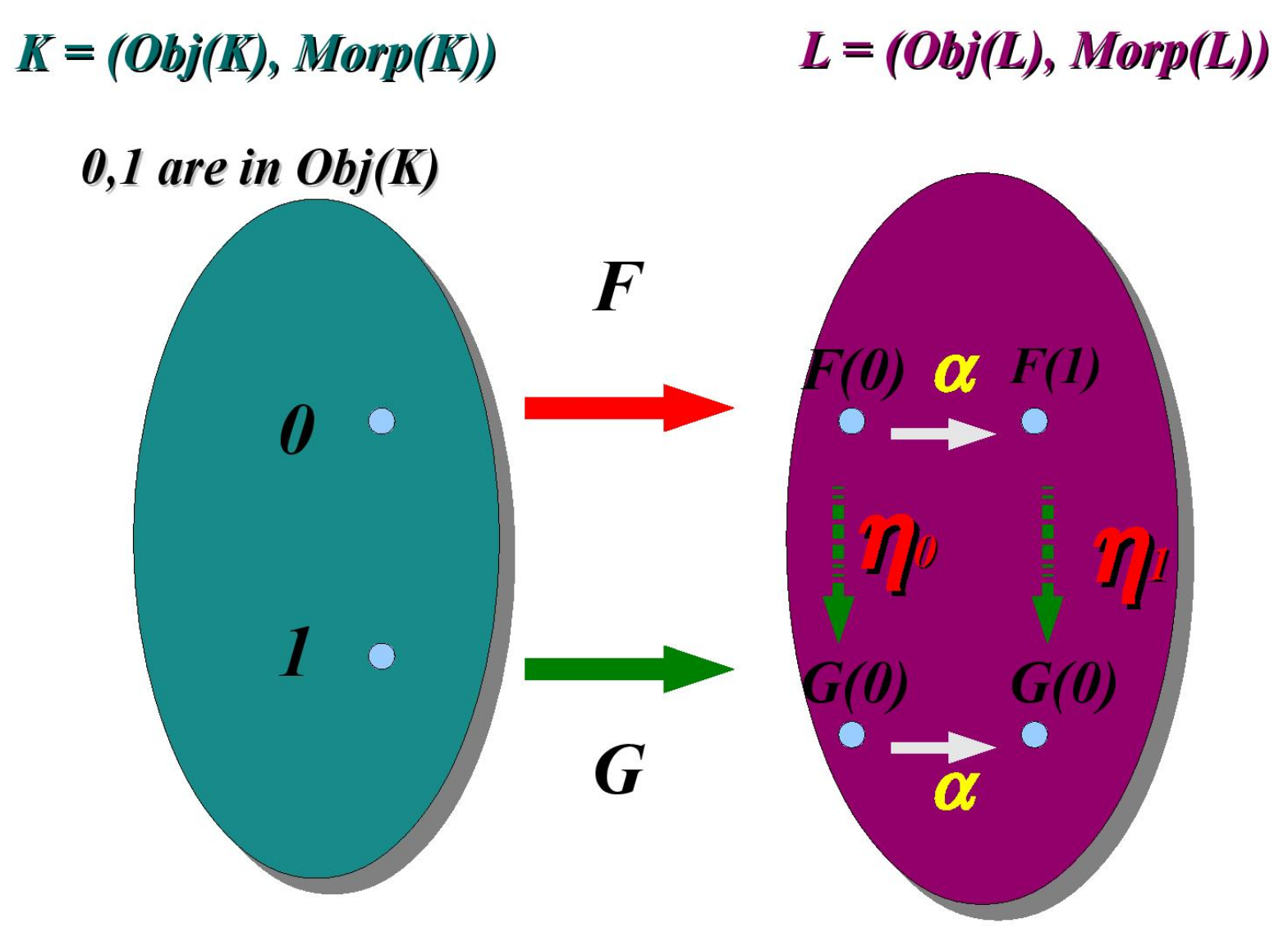
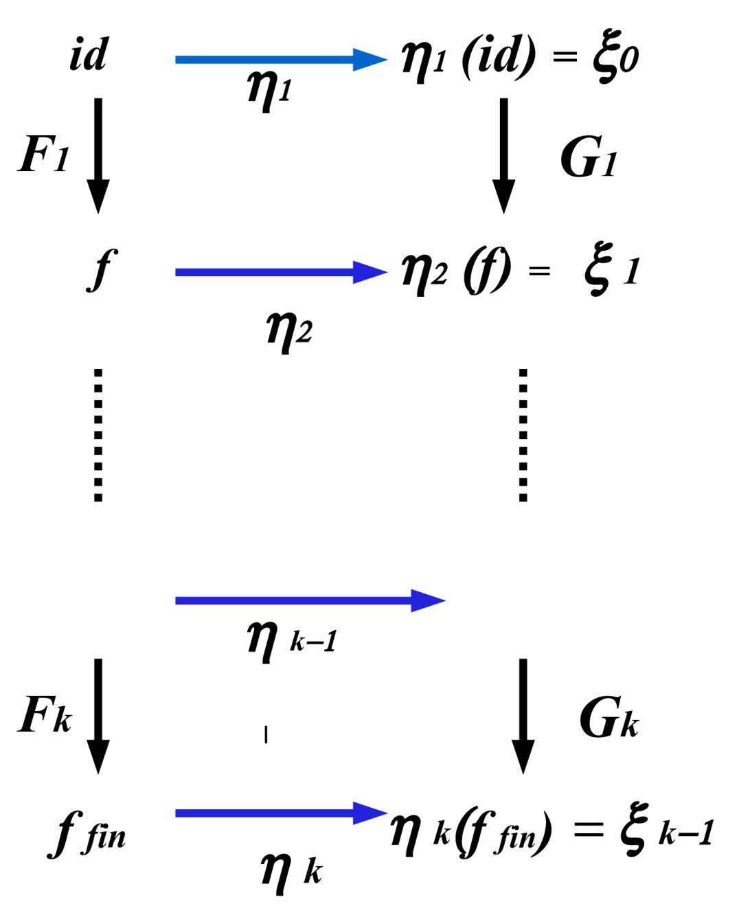
Let us assume that two categories
K and
L and the functors
F and
G:
are given (see:
Figure 1). Independently of their nature (either a covariant or a contravariant one), one could transform (map)
F into
G (see:
Figure 1 and
Figure 2). In this way, the so-called
natural transformation may be defined between
F and
G (It is represented by a pair of components
in
Figure 1). Its rigorous definition is as follows.
Definition 6. Let us assume that two categories and and two functors F and G are given. Then a natural transformation (from F to G) forms a family of such mappings, which satisfy the following two conditions:
- (a)
to each object a morphism in D is associated (it forms a component on η at X).
- (b)
It holds the commutativity: .
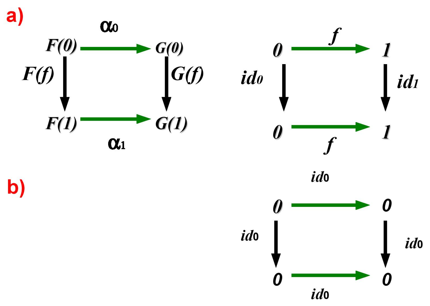
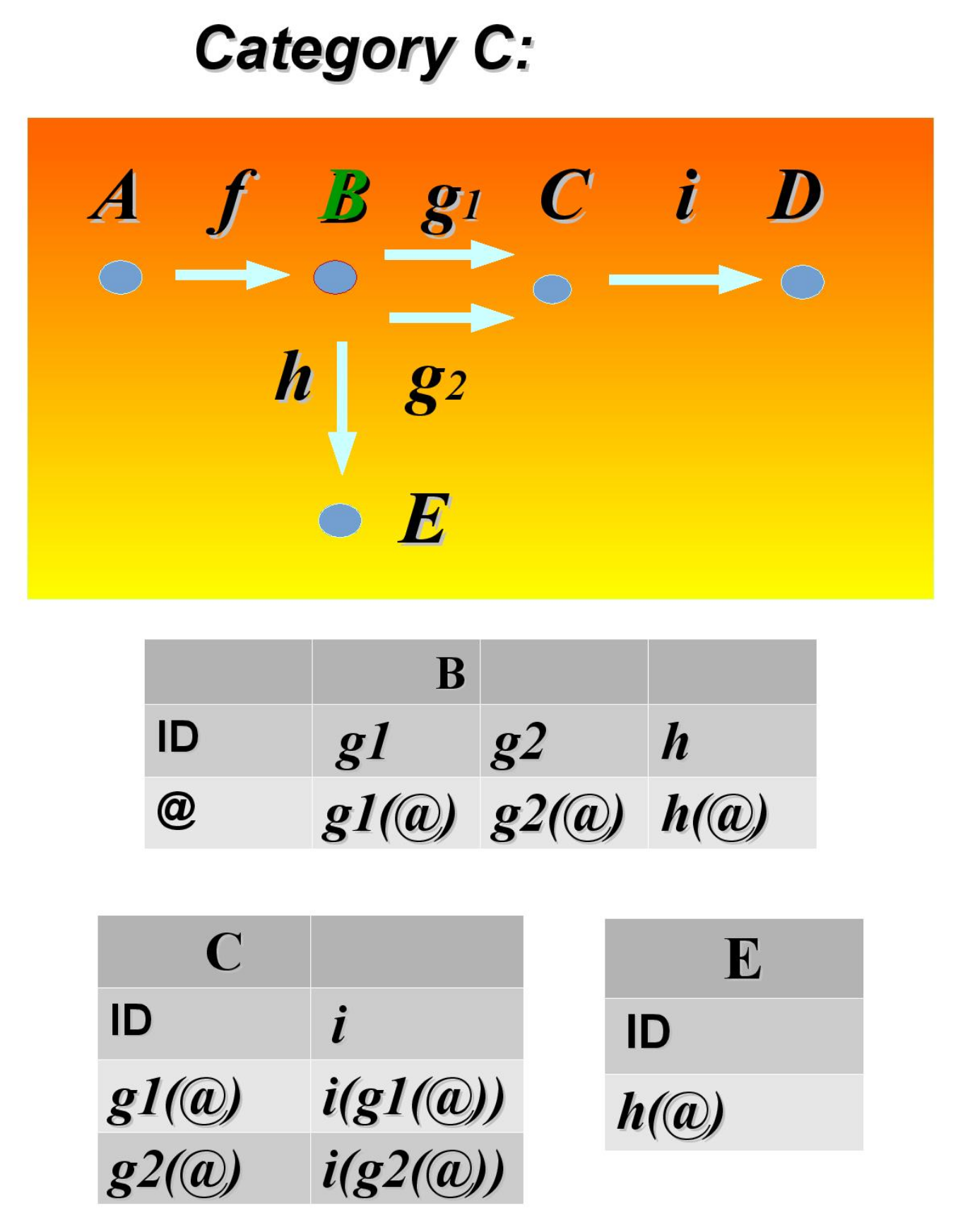
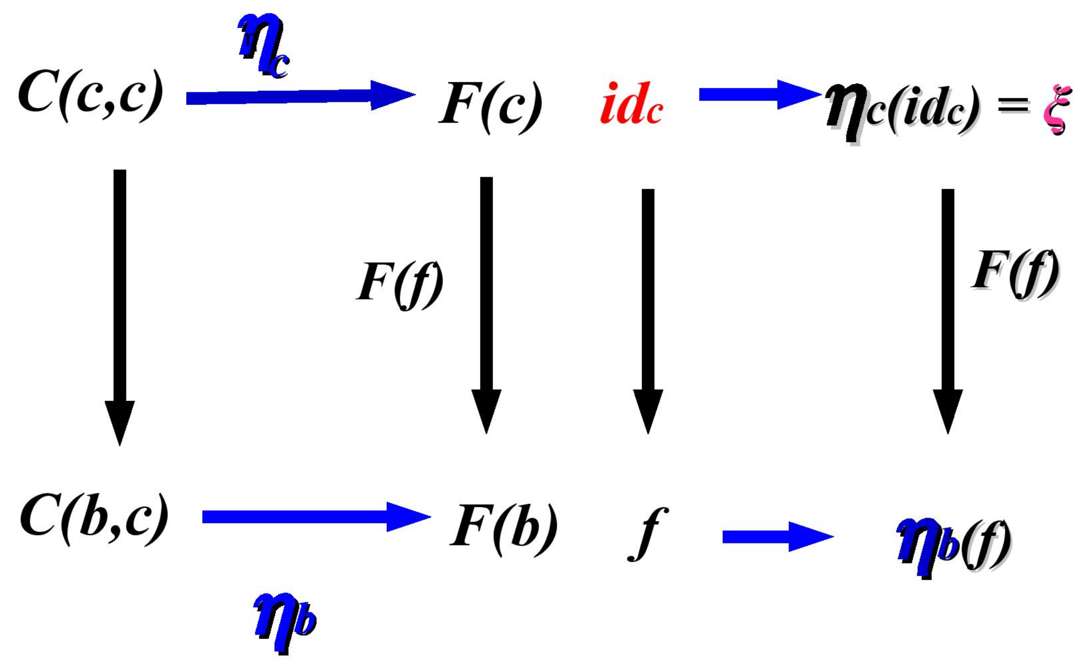
Example 5. Let us consider two functors F and G (operating between categories and )–as presented in Figure 2a) (see: the upward diagram) provided that –as in Figure 2a) (see: the right diagram). The components of the natural transformation (only possibly in this case) are: , because such a defining way guarantees that the diagram commutes. Meanwhile, if and , the only admissible association is , (see: diagram 2b)). The next example is in Figure 3. Definition 7. (Representable functor) Let us assume that forms a (locally) small category It does not mean that the category is small. Let also , for each object , be the so-called hom-functor, which maps object X to the set (set of homomorphisms from A to X). Then a functor is a representable functor for if it is naturally isomorphic to , for some A of . The representation of F is given by a pair , for: Example 6. Let us take into account a category with as its objects and a couple of morphisms between them as presented in Figure 3. All the hom-functors: and are determined here by the following tables. Theorem 1. (Yoneda’s Lemma) Let assume that is a locally small category, let be a hom-functor, for each object and let F be a functor from Sets. Then the natural transformations η from to F is a one-to-one (bijective) correspondence with the set , i.e., The formulation of Yoneda’s lemma itself delivers an operational guideline how to predict a form of a natural transformation between a given functor
F and its Hom-functor. In fact, you need to know
F-value for the the initial object
(see:
Figure 4).
The proof idea: The core of the proof relies on the demonstration of the fact that the entire transformation may be fully determined by a single value , for any object . For the proof of the fact, a naturality of will be exploited.
The diagrams in
Figure 4. show that not only
may be determined by
, but also
as
. In the similar way, we are in a position to determine the natural transformation
for other initial objects of
. It finishes the proof. The illustration of the leading problem is in
Figure 5.
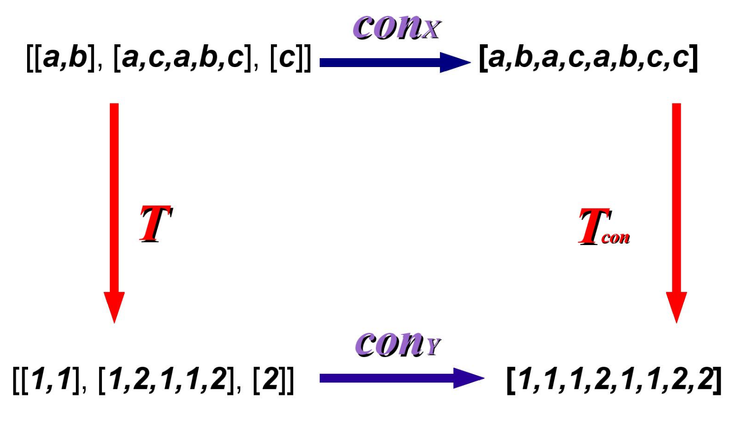
2.2. The Leading Problem Formulation
Let us consider the following list:
(with elements being lists:
and
). Let us assume that the list is transformed in a horizontal dimension (by a concatenation functor
) and in the vertical dimension (by a translation
T)–as depicted in
Figure 5. Let also assume that the concatenated list [a,b,a,c,a,b,c,c] will be transformed horizontally by
translation and the translated list [[1,1],[1,2,1,1,2],[2]] will be concatenated vertically by
. After the whole procedure–in both cases–the same final list
is obtained because of commutativity of the diagram. Let us decide the following problems.
- A
How to fuzzify (i.e., to violate the commutativity of the diagram for) the natural transformation between functors and ,
- B
What is the effect of defuzzification of the transformation?
- C
How to manage correctness (lack of errors) of the translation if the translation process will be continued up to k-stage It means that the corresponding multi-diagram contains k single diagrams. will be constructed?
- D
How to control the errors in exemplary scenario after 3 multi-diagram stages if the pairs of sets (achieved by the upward and the downward functor composition) are as follows:
and –after the first stage,
and –after the second stage and
and –after the third stage ?
3. The Natural Transformation Based on Fuzzified Commutativity
Before moving to the right part of the paper analysis to define a multi-fuzzy natural transformation, let us recall the observation that the natural transformation is defined by commutativity of the appropriate diagram. Obviously, the diagram commutativity–defining the natural transformation–is uniquely represented by the following equation (see: the proof for Yoneda’s lemma):
This equation might be read as follows: there exist two alternative paths from an initially chosen object
to the final points of the diagram transformation. The first path is determined by the composition
with
f-mapping. The alternative second way–by the composition functor
for
as the functor argument (see:
Figure 4, the right diagram).
The authors of [
20] observed that one of the most promising way of the commutativity fuzzification takes into account either the embedding:
Indeed, the inclusions in (6)–as a form of some relaxation of the original Equation (
5)–introduce a kind of fuzzification of commutativity–as given by (5). The inequality introduces a new situation of a difference (relative) set. In this way, the following types of relative sets are possible (/ is a usual set-theoretic difference between two sets):
,
, and A forms a finite set,
, and A forms a denumerable set,
, and A forms a uncountable set.
Obviously, the empty set (case 1) is associated to the usual diagram commutativity. The (case 2) determines the situation of each arbitrarily large, but finite set. It is also clear that the (case 3) refers to all sets, which are equinumerous with the set of natural numbers.
The fact that either the first or the second inclusion in (6) hold and the existence of different types of relative sets (dependent of their cardinality) motivated the authors of [
18] to introduce different subtypes of fuzzy natural transformations. Nevertheless, a distinction for the ‘upward’ and the ‘downward’ fuzzy natural transformations was a basis of their taxonomy Different types of fuzzy natural transformations were introduced in [
20]: the finite-valued (upward/downward) and their denumerable and uncountable counterparts. Informally speaking, the upward fuzzy natural situation forms such a variant, in which the ‘upward’ diagram composition of the functors gives a a ‘greater’ set than the set obtained via the ‘downward’ functor composition. It was formally introduced in [
18] as follows. (Its multi-valued variants modify the definitions from [
19].)
Definition 8. (The upward fuzzy natural transformation) The name of this type of transformation is motivated by the fact that the result set achieved by the composition (see: Figure 6 or Figure 7)–has a greater cardinality than the set achieved via the downward composition..) Let us assume that two categories and together with the functors F and G are given. Then the upward fuzzy natural transformation η between F and G forms a family of mappings such that the following conditions are satisfied: Towards a Multi-Fuzzy Natural Transformation
In this part, a multi-fuzzy natural transformation–as en extension of the constructions from [
20] is put forward. For a use of the construction, let us assume that a single diagram for fuzzy commutativity– as the right diagram in
Figure 4—is given. Let us enlarge this diagram to a multi-diagram—as presented in
Figure 6.
A novelty of the situation is based on occurrence of two sequences of functors: and instead of a single pair of functors F and G, for . In consequence, a sequence of the following values was obtained, where–as previously–, but also , etc.
By analog to the usual natural transformation–one can identify a multi-natural transformation (still a non-fuzzy one) with a sequence of mappings
, for a fixed finite
k. Obviously, each of the element of the sequence forms a component of the natural transformation. These components guarantee that the most external diagram in
Figure 6 commutes, i.e.,
.
The most natural way to introduce a piece of fuzziness to the multi-natural transformation is to exchange the sequence of equalities (defining a ‘global’ commutativity of the multi-diagram) for a sequence of inequalities. It only remains to decide whether the result set of the ‘upward compositions’ of functors is included in the result set of the ‘downward’ path or conversely One can generalize this criterion in order to adopt a method to compare the set cardinalities. Nevertheless, this manoeuvre seems to be too radical and introducing some elusiveness. Moreover, considering the cardinalities of the sets might be somehow misleading for measurement of fuzziness, if the measurement refers to the result sets with an empty common intersection.
Simultaneously, we can expect that the final relative sets–obtained as such cumulative sets from the intermediate relative sets–will preserve a piece of information about a provenance of all elements. Therefore, we are rather willing to express the final relative sets in terms of simple sums of the intermediate relative sets. (This solution will be also useful in a proof of the new multi-fuzzy Yoneda’s lemma.) More formally, if assume that is a sequence of all consecutive relative sets is associated to the first diagram of a given k-multi-diagram, –to the second one, etc., then the final relative set A (obtained after k stages in k-multi-diagram) is given as .
All these establishments lead to the following variants of multi-fuzzy natural transformations.
Definition 9. (The upward multi-fuzzy natural transformation As in [20], the name–as previously–was motivated by the observation that the composition by the upward diagram part gives the set of values with a cardinality greater than –obtained by the downward diagram part.) Let us assume that a finite sequence of categories with two corresponding sequences and of functors operating between the categories are given, for a finite k and . Then the upward multi-fuzzy natural transformation η from to forms a family of mapping such that the following requirements are satisfied: to each object a mapping in is associated (it forms an i-component of η at X), for .
it holds the upward fuzzy commutativity: (the result set of the ‘upward’ functor composition contains the result set of the ‘downward’ composition of the functors.)
Definition 10. (The downward multi-fuzzy natural transformation.) Let us assume that a finite sequence of categories together with two corresponding and finite sequences and of functors operating between the categories are given, for . Then the downward multi-fuzzy natural transformation η from to forms a family of mappings such that the following requirements are satisfied:
to each object a mapping in is associated (it forms an i-component of η at X), for ,
it holds the downward multi-fuzzy commutativity: (the result set of the ‘downward’ functor composition contains the result set of the ‘upward’ functor composition.).
The possible classes of cardinalities of the relative sets differentiate both the ‘upward’ and the ‘downward’ fuzzy natural transformation–dependently on the cardinality of the relative set. We restrict defining the cases for the ‘upward’ cases. In fact, their downward variants are defined by analogy.
Definition 11. (The finite-valued upward multi-fuzzy natural transformation.) Let us assume that a finite sequence of categories and two corresponding and finite sequences of functors operating between the categories (resp.) are given, for . Then the finite-valued upward multi-fuzzy natural transformation η from to forms a family of such the mappings that the following requirements are satisfied:
to each object a mapping in is associated (it forms an i-component of η at X), for ,
it holds the upward multi-fuzzy commutativity:
and the relative set A determined by (9) is finite (it satisfies the condition ).
In a same way, not only the denumerable-valued upward multi-fuzzy natural transformation, but also the uncountable-valued upward multi-fuzzy natural transformation may be introduced.
Definition 12. (
The denumerable-valued upward multi-fuzzy natural transformation.)
Let us assume that a finite sequence of categories together with two corresponding sequences of functors and operating between the categories (resp.) are given, for . Then the denumerable-valued upward multi-fuzzy natural transformation η from to forms a family of mappings such that, these requirements are satisfied:
to each object a mapping in is associated (it forms an i-component of η at X), for ,
it holds the upward multi-fuzzy commutativity:
and the relative set determined by (10) is denumerable, i.e., .
Definition 13. (The uncountable-valued upward fuzzy natural transformation.) Let us assume that a finite sequence of categories together with two corresponding sequences and of functors operating between the categories (resp.) are given, for . Then the upward multi-fuzzy natural transformation η from to forms a family of such mappings that the following requirements are satisfied:
to each object a mapping in is associated (it forms an i-component of η at X), for ,
it holds the upward multi-fuzzy commutativity:
and the relative set determined by (11) is equinumerous with the set of real numbers, i.e .
4. The Natural Transformation with Multi-Fuzzy Commutativity in Terms of Hamming’s Distances
From an operational and application-based perspective–it may be interesting which types of multi-fuzzy natural transformations preserve a computational nature (if any). Fortunately, the answer to the question may be positive–such a convenient property forms a feature of all ‘countable’. In [
20], all countable situations were described by means of coding theory by their reference to Hamming’s distances. This solution enabled us to distinguish another subclass in the broad taxonomy of the multi-fuzzy natural transformation: the class of Hamming’s countable-valued fuzzy natural transformations. The idea to render countable cases of multi-fuzzy natural transformations by means of Hamming’s distances and other terms of coding theory stems from an observation that all relative sets in these countable cases may be viewed as the result sets of an error coding (an error word transmission). Formally, the difference/relative sets (in the countable cases) have been identified with sets
–the sets of all indices
i, for which
a =
and
in
remain mutually different.
This leads to the following definition of Hamming’s countable-valued upward fuzzy natural transformation.
Definition 14. (Hamming’s countable upward fuzzy natural transformation, see: [20].) Let us assume that two categories C and D together with two functors between them are given. Let us also assume that forms an upward fuzzy natural transformation. Then η is Hamming’s countable-valued upward fuzzy natural transformation provided that the following condition:is satisfied and either or . Otherwise, if
is already considered instead of
the
Hamming’s countable-values downward fuzzy natural transformation may be defined.
The same founding idea and the same conceptual tissue with definitions of Hamming’s distance and Hamming’s ball(see: [
21], pp. 375–378) are incorporated to the Hamming’s countable upward/downward multi-fuzzy natural transformations.
Definition 15. (See: [21].) Let Σ be a finite alphabet and the words a = , , for some fixed . Then the Hamming’s distance between words a and b in is a cardinality of the set . We write is . Definition 16. (See: [21].) The Hamming’s ball of radius d and a center a is the following set Theorem 2. (See: [21].) The following condition defines the necessary and sufficient condition to detect at most d errors.
Meanwhile, it remains to solve the problem of effective computing the final relative sets (obtained from the intermediate relative sets). As previously described–we are convinced to render the final relative set by means of the simple sum of the intermediate relative sets In fact, this solution enables us to preserve a piece of information about the provenance of all the elements of the final relative set.
Therefore, let us consider a
k-multi-diagram This is a multi-diagram with
k-single diagrams.–as in
Figure 6 (or
Figure 7). If
constitute all consecutive relative sets for the 1-st, 2-nd, …,
k-diagram, then the final relative set
A after these
k-steps is determined by the simple sum of them, i.e.,
Let us note that the following identification
with
is admitted because of finiteness of the simple sum.. The formal definition is the following.
Definition 17. (Hamming’s countable downward multi-fuzzy natural transformation) Let us assume that a finite sequence of categories together with two corresponding finite sequences and of functors between them are given, for . Then Hamming’s countable upward multi-fuzzy natural transformation η from from forms a family of such morphisms that the following requirements are satisfied:
to each object a morphism in is associated (it forms an i-component of η at X), for ,
for each in Let us observe that we have exactly relative sets as the result of single diagrams if the number of η-components is k., where
This way of defining also delivers a criterion of recognizing whether a given multi-fuzzy natural transformation is of the Hamming’s sort. This fact is simply determined by the cardinality of the most ‘greater’ sets from their simple sum It is noteworthy that this comparison works perfectly for finite sets only. In fact, denumerable sets cannot be perfectly distinguished by considering their cardinalities. Other topological properties of them, such as density or nowhere-density, should be taken into account. In order to define the upward counterpart, it is enough to change the order of the functor compositions in the set difference on the right side (19).
5. Fuzzy Yoneda’s Lemma
Having introduced a complete taxonomy for a variety of the multi-fuzzy natural transformations, we can venture to formulate the corresponding multi-fuzzy Yoneda’s lemma.
Let us recall the fact that the discrepancy between the original Yoneda’s lemma and its fuzzy counterpart–due to [
20]–manifests itself by a
degree of similarity between the Hom-functor
and its representable functor, say
F. Indeed, we deal with an isomorphism in the original Yoneda’s lemma and with a similarity ∼ (measured by the cardinality of difference sets)–in fuzzy Yoneda’s lemma. In the last case, we think about
similarity up to the difference set A denoting it as ‘
’.
It is clear that the multi-fuzzy Yoneda’s lemma should also be based on a kind of a multi-similarity (). Besides, a method of defining the final relative sets (in this new multi-fuzzy situation) by a simple sum of the intermediate relative sets should also be reflected in the new definition.
Definition 18. (Multi-similarity up to the difference set A.) Let be two arbitrary sets. It will be said that K is multi-similar toM up to d.s. A if and only if , where for some , for a fixed k In practice, we only consider finite simple sums. We will write (up to d.s. A). Conversely, we say that M is multi-similar to The sens of the name may be explained by the fact that each finite simple sum might be identified with the sequence of its components. K up to the difference set A if and only if , and A forms a finite simple sum of some components.
It enables us to give a precise formulation of the multi-fuzzy Yoneda’s lemma. It is not difficult to see the main discrepancy between fuzzy Yoneda’s lemma and its multi-fuzzy version. It relies on the fact that the pairs (consisting of a given functor and its representable functor) are exchanged for the finite sequences of functors and their representable functors.
Theorem 3. (The multi-fuzzy Yoneda’s Lemma.) Let assume that be a sequence of locally small categories and let be a sequence of functors from Setsand let –be the hom-functor for . Then the downward fuzzy natural transformations η between and is similar to the set up to d. s. A, and we will denote this fact by: for i = 1,2…, k.
An outline of the proof: The proof runs by induction over the complication degree of the multi-diagram.
The objective of the proof–due to the original proof of the classical Yoneda’s lemma–is a task to predict the form of all the components of the fuzzy natural transformations.
Therefore, let us assume that
be an initial category
,
are two fixed objects of
(as in
Figure 4), and let also assume that the functor
F and
and
are given to establish two components
and
of
-transformation. As previously, an initially chosen object
is transformed via
(the first transformation path). Having established the values
as
, we can obtain by
, i.e., the value
. Simultaneously,
is transformed via
f composed with
, i.e.,
(the second transformation path). If
forms the upward fuzzy natural transformation, then
. Hence–due to Def. 18–
. In this way
has been established by
, excluding the points of difference set
A. Hence:
The same reasoning might be repeated for the downward variant. If
, i.e., when we deal with a single fuzzy diagram, the proof runs as presented in [
20]. For
(see:
Figure 7) we can exploit the fact that each such a
–from
up to
–may be established to execute the similarity
(up to d.s
because–at each diagram stage–the functors
and
(for each
) satisfy the same assumptions as the pair
F and
-functor from the classical Yoneda’s lemma. Indeed, it is enough to restrict the proof analysis to these elements, for which the diagram commutes (obviously - we should omit the points from relative sets). After establishing
, it is not difficult to define the final
and to repeat the previous reasoning to find the last component
as previously. It exactly means that we determine the following similarities:
, at each stage
i of the multi-diagram-based construction. Finally, the thesis of the theorem may be deduced from it and from the fact that
is achieved by composing
.
6. The Problem Solving and Closing Remarks
Having defined fuzzy natural transformations by means of Hamming’s distances, we can venture to return to our initial problem in order to find the answers to the questions A, B, C, and D.
Ad. A. According to the previous results from Section IV–a possible fuzzification of the natural transformation
should be identified with similarity up to d. s.
A for the relative set
, for
(see:
Figure 5). Because the finally obtained lists [1,1,1,2,1,1,2,2], [1,1,2,3,2,2,1,1]–in the Hamming’s representation–may be identified with the words
a =
and
b =
(over
) by Hamming’s distance
. Obviously, the lists remain different in 6 places, thus their
.
Ad. B. In our case, a defuzzification process (returning to the non-fuzzy natural transformation) requires to detect all the 6 errors. The necessary and sufficient condition of an error detection (for at most d errors) indicates that the condition (15) should be verified. As the lists a, b are mutually different, one only needs to check whether . However, , thus , so the fuzzification process is not feasible for that pair. Hence, a pair of lists with at least 7 different values is required.
Ad. C It has already been said that the simple sum-based construction of the final relative sets (over a given multi-fuzzy diagram) does not lose any piece of information about the provenance of the set elements. In other words, we are in a position (at each i-stage of the k-multi-diagram analysis) to indicate the intermediate relative set, from which a given element is taken. Simultaneously, each relative set in the final simple sum, for , may be seen as a result of the error propagation at an i-stage (diagram) of the k-multi-diagram. Thus, the final error propagation A over the whole multi-diagram is controllable by considering the simple sum .
Ad. D Let us initially assume that the initial lists of points (after each stage), i.e., [1,1,1,1,1,1], [1,1,2,0,0,0] and [1,1,0,0,0,0] have been obtained via the downward composition of the appropriate functors. Let us also assume that we are interested in the relative sets as a difference between the , where is an ‘upward composition’ set (after an i stage) and is a ‘downward composition’ set (after an i stage), for It is also noteworthy that a kind of a pattern of correctness must be established here in order to solve the case. In our case, the ‘downward composition set’ plays such a role. Meanwhile, the ‘upward composition’ set is considered as the modified one with potential errors to be detected. This establishment plays a role of a feasibility criterion for the task.. In other words, we need to detect the relative sets and after each diagram stage. For clarity we will mark the places where the corresponding values are different, by letters , where informs about the place of the error in the order of errors of a given list, and denotes the diagram stage.
By the assumptions and after the appropriate computing we get:
,
,
,
Due to the points C–the final error propagation relative set A is given as .
7. The State-Of-The-Art
This paper research forms a slight and more detailed extension of research from [
19] and initially stems from [
18], where a concept a fuzzy natural transformation was introduced and described for single non-commutative diagrams.
Although these papers contain purely theoretic results–they are rather practically motivated, what found its reflection in describing some selected combinatorial aspects of the paper issue concerning the error detection criteria. In this perspective–these papers do not participate in the recent debates on a category-theory based foundations of set theory and its fuzzy counterpart–against many articles, such as the works collected in seminal monographs [
12,
22]. The papers of this sort are often aimed at the proposing the most proper and mathematically rigorous categorial semantics for fuzzy set theory, as proposed in terms of Takeuti-Titani’s models from [
23] (see also: [
24])–due to [
25]–and recently in [
26] in terms of the so-called fibred algebra.
The methodological differences between the papers collected in [
12] and the papers [
18,
19] manifest in approaches to the issue of fuzziness in its relation to category theory. While the papers from the monograph propose mainly a kind of a categorial depiction of different –sometimes sophisticated–mathematical objects (subobjects of the so-called SM-SET algebras in [
13]), spaces (fuzzy topological spaces in [
14]), theorems or theories (Stone Representation Theories in [
27]), the papers [
18,
19] give a fuzzy and multi-fuzzy modification of a purely categorial concept of natural transformation.
The same paradigm of fuzzification of some mathematical (mostly: for the algebraic and graph theory-based) objects was incorporated in several previous papers, such as [
9]) (for fuzzy groups), [
10] (for fuzzy graphs) or [
11] (for C*-algebras). Although an idea of fuzzification of purely categorial objects–to the best of the author’s knowledge–has not been yet materialized directly, some papers elucidated a fuzzy ‘face’ of some categorial objects, such as in [
28], where the category of sheaves over a complete Boolean algebra
B is interpreted as equivalent to the category of
B-valued sets and maps (in the Scott-Solovay sense).
The concept of fuzzified natural transformation itself seems to show some similarity to the so-called
m-polar fuzzy sets–recently described as a natural enlargement of the so-called bipolar fuzzy sets in [
29] and extended towards ideals of BCK/BCI-algebras in [
30] and the so-called
m-polar fuzzy graphs in [
31]. In fact, the construction of
m-polar fuzzy sets–as illustrated in [
29]–preserves a piece of information about the provenance of elements in the set. The same property may be associated to the final relative sets–given by the simple sums of the
i-stage intermediate relative sets. In addition, both fuzzy natural transformations and
m-polar fuzzy sets constitute essentially a collection of the appropriate mappings from an initially given set. Simultaneously, the images of the mapping defining
m-polar fuzzy sets (the
m-products of the compact interval [0,1]) are considered as the lattice-type structures, what introduces a difference between them and relative sets, which form purely set-theoretic collections of objects without any additional algebraic structures imposed on them.
Meanwhile, the m-polar fuzzy sets constitute the twin entities for the so-called multi-fuzzy sets. The last ones are determined by the so-called multi-membership functions–they form the sets of sequences consisting of the appropriate membership functions (for arguments taken from an initial non-fuzzy set) The formal and general definition in terms of complete lattices is the following one.
Definition 19. Let X be a non-empty set, let be the set of all natural numbers and let be a set of complete lattices. Then a multi-fuzzy set A (in X) forms a set of the sequences (see: [32], p.37): and , for each .
This way of defining these entities and a lack of polarity determines the main discrepancy between them and
m-polar fuzzy sets, which also manifests itself by the method of their algebraic depiction. Whereas
m-polar fuzzy sets are conceptually based on simple sums, the multi-fuzzy sets are expressible in terms of ordinary sums This property seems to be especially visible for some unique types of the multi-fuzzy sets, such as the multi-fuzzy sets with linearly dependent infinite coordinates. Indeed, such a set, say
A, is defined as follows. (See: [
32], p. 37.)
In this way, the multi-fuzzy transformations should be conceptually located between the m-polar sets and the multi-fuzzy sets.
8. Closing Remarks
It has been just illustrated how to construct a variety of the multi-fuzzy natural transformations based on a fuzzy natural transformation. The main distinction criterion–adopted to elaborate the frame of this taxonomy–was a cardinality of the newly introduced difference sets. We are in a position to elaborate the Hamming’s distance-based depiction of the multi-fuzzy natural transformations with respect to finite or denumerable difference sets. An additional novelty of the paper analysis constitutes the multi-fuzzy Yoneda’s lemma. Its formulation with its proof outline was put forward. Due to our expectations–it enables us to forecast a form of multi-fuzzy natural transformations. However, this task is only approximately feasible. We have proposed to describe this fact as similarity ‘up to the difference sets’. Whereas an original Yoneda’s lemma allows us to forecast a general form of the natural transformation for a pair of functors, the multi-fuzzy Yoneda’s lemma enables us to predict the form of the corresponding multi-fuzzy natural transformation for a chosen finite sequence of functors. One can venture into a thesis that the multi-fuzzy Yoneda’s introduces some portion of optimism. Indeed, the construction of the multi-fuzzy transformation over the corresponding multi-diagram allows us to preserve a piece of knowledge about the relative difference sets’ provenance. However, the presented approach seems to be having some important restrictions. In fact, the idea of fuzzification of natural transformations–since it bases on a finite multi-diagram–cannot be incorporated for natural transformations–based on arbitrarily large multi-diagrams. It corresponds to a well-known non-extendability of some mathematical properties from the finite cases for the infinite ones.
Simultaneously, category theory seems to constitute convenient machinery to elucidate and generalize an algebraic nature of the code error detection–due to their combinatorial taxonomy (for Hamming codes, Hadamard codes, or Reed-Muller codes). Independently of this issue–one can venture to formulate an optimistic thesis that these theoretic considerations might find their possible application area in some programming-based frameworks of Erlang or Haskell.
It seems that the paper constructions may refer to many different structures. Obviously, the world of the categories themselves, such as Set, GR, Top, Metr and their mappings do not exhaust the class of all entities, which may be modeled by them. It seems that some structures and the diagram-based relations of a linguistic nature may constitute an attractive application area of the paper constructions and theoretic considerations. It has been shown how the multi-fuzzy diagrams work in the word error detection, this—in the context of lexis of formal languages. Meanwhile, many categorial diagrams may be exploited to represent the appropriate (parts of) derivation trees in the natural language sentences’ syntax analysis. If a single diagram can represent a phrase of a single sentence, the appropriate and modified multi-diagrams may be potentially exploited to represent broader fragments of statements. This idea seems to be a promising area of future exploration.
Last, but not least–the mutual relationships between relative sets and m-polar fuzzy sets seem to extend a potential application area of the first ones in computer science towards such entities as multi-agents, multi-attributes, multi-polar information, or uncertainty. However, all these ideas also require a deeper analysis.


