1. Introduction of Ontology and Ontology Learning
Originally, ontology was derived from a philosophical concept in ancient Greece, an essential science in the study of the existence of things. Ontology abstracts the concepts of things to describe the detailed characteristics of things. In recent years, this concept has been widely applied to the field of information technology, especially in artificial intelligence, semantic web and bioinformatics. The definition currently accepted by most scholars is “a formal specification of a shared conceptual model.” Conceptual model refers to an abstract generalization of things in the objective world; formalization refers to the existence of the conceptual model in a computer-understandable form; sharing refers to the concept expressed by the conceptual model recognized and acquired by the public, reflecting commonly recognized concepts in related fields; norms refer to the definition of these concepts which are clear and multi-level. The core idea is to define concepts in the field and the relationship between concepts, and to make the reuse and sharing of concepts possible. Ontology is a semantic carrier for communication between different subjects, and mainly discusses the formal representation of concepts, whose core is a conceptual model in the field of computers. Ontology provides the formalization of concepts in the domain and the relationship between concepts, and it is a special set of concepts that can be understood and solved by a computer so that the computer can understand the semantic content. Several ontology-related contributions and their applications can be referred to Lv and Peng [
1], Lammers et al. [
2], Jankovic et al. [
3], Geng et al. [
4], Li and Chen [
5], Angsuchotmetee et al. [
6], Shanavas et al. [
7], He et al. [
8], Hinderer and Moseley [
9], He et al. [
10].
Ontology components include:
Individuals: also called examples;
Category: abstract representation of concept sets;
Attribute: the characteristics of the class;
Constraint: also called restriction;
Functional terminology: an abstract representation of specific terms in mathematical expressions;
Rules: statements in the form of antecedent and consequence statements;
Axiom: a statement that is asserted as a priori knowledge.
Ontology can be divided into top ontology, domain ontology, task ontology and application ontology according to usage scenarios:
Top ontology: describing concepts and relationships among concepts that are common in all domains;
Domain ontology: expressing the terminology of a specific domain, and comprehensively describing the characteristics of the domain;
Task ontology: the set of concepts needed to solve a specific task;
Application ontology: describing concepts and relationships between concepts that depend on specific fields and tasks.
Ontology has the characteristics of sharing, reuse, and semantics contained. It can describe knowledge in a formal language that can be understood by machines, and solve the barriers of information and knowledge exchange between people and machines, and between machines. Ontology can provide a clearly-defined set of concepts, and a semantically consistent communication medium between subjects (human and human, human and machine, machine and machine).
As the amount of data processed by the ontology has increased, the structure and data types of the ontology have changed greatly compared with the past. The original traditional heuristic ontology computing method is no longer suitable for computing tasks in the context of big data. Therefore, ontology learning algorithms are widely used in ontology similarity calculation, ontology alignment and ontology mapping. The so-called ontology learning is to use the tricks of machine learning to merge with the features of the ontology, obtain the optimal ontology function through the sample, and then get the ontology similarity calculation formula. A common strategy is to yield a real-valued function, map the entire ontology graph to a one-dimensional real number space, and then use one-dimensional distance to judge the similarity between ontology concepts. Furthermore, consider that the graph is the best choice to express the dada structure and, in most cases, the structure learning can be transformed into the graph learning, the graph learning is raising big attention among data scientists. As a tool for structured storage of data, there are various connections between ontology concepts, and thus using graph structure representation is the best choice. When using a graph to represent an ontology, the definition of edges in the ontology graph is the most critical, and it can determine the type and strength of connections between concepts. It is logical that graph learning algorithms that consider the characteristics of graph structure itself in the learning process naturally attract the attention of ontology researchers.
In recent years, there are some advances obtained in ontology learning algorithms and their theoretical analysis. Gao et al. [
11] raised an ontology sparse vector learning approach by means of ADAL technology which is naturally a kind of ontology sparse vector learning algorithm. Gao et al. [
12] determined a discrete dynamics technical to sparse computing and applied in ontology science. Gao et al. [
13] suggested a partial multi-dividing ontology learning algorithm for tree-shape ontology structures. Gao and Farahani [
14] calculated generalization bounds and uniform bounds for multi-dividing ontology algorithms in the setting that an ontology loss function is convex. Gao and Chen [
15] gave an approximation analysis of the ontology learning algorithm in a linear combination setting. Zhu et al. [
16] discussed the fundamental and mathematical basis of the ontology learning algorithm. Zhu et al. [
17] considered another setting of the ontology learning algorithm where the optimal ontology function can be expressed as the combination of several weak ontology functions.
The biggest difference between ontology and other databases lies in that ontology is a dynamically structured database for concepts. Compared with the single record of other database structures, ontology uses a graph structure to represent the relationship between concepts, and at the same time, different ontologies interact in light of ontology mapping. Therefore, we often regard ontology learning as learning on ontology graphs, and graph learning algorithms are applied to ontology learning.
In order to express the learning algorithm conveniently, it abstracts the relevant information of the ontology concept, which is to encapsulate the names, attributes, instances, and structure information of the concept with vectors. As a result, the components of the target sparse vector also contain some special structural features, such as symmetry and clustering. In many application scenarios, like genetics, such vectors often have a large dimension. However, in a specific ontology application background, only a few components are important or can make a difference. For example, while diagnosing genetic diseases, there are actually only a few genes related to such diseases, and the others are not important. In this way, the learning goal is to find a few genes related to the disease among a large number of genes. When it comes to ontology applications, for a specific ontology application scenario, we often find that it is only related to a certain part of the information in the conceptual information. For example, in the GIS ontology, if an accident like a robbery occurs in a university, we only need to find a police station or a hospital near the university; if for eating and shopping, we only care about the restaurants and supermarkets near the university; if we go outside, we must concern ourselves about the subway station near the university. For different application backgrounds, we will pay attention to different components in the ontology vector information, and each application is only related to a small amount of information (corresponding to a small number of components in the vector). This makes sparse vector learning extra important in ontology learning.
In a sense, the goal of ontology sparse vector learning is to determine the decisive dimensional information from a large amount of cumbersome high-dimensional data space according to the needs of a certain practical application, and thus it is a dimensionality reduction algorithm. When p is large, this type of algorithm can effectively lock the components of the ontology vector that play a decisive role, thereby greatly reducing the computational complexity in the later stage.
In addition, considering that the graph is an ideal model for representing the structure of the data, it can represent the internal relationships between elements and the overall structure of the entire data. In fact, ontology and knowledge graphs are good examples, making full use of graph structures to express the connections between complex concepts. Therefore, each component in the ontology sparse vector represents the information of the ontology concept, and the correlation between them can also be represented by a graph structure. The graph learning is used to effectively integrate the features of the graph structure into the machine learning algorithm, such as spectral information.
In this work, we discuss the ontology learning algorithm in the ontology sparse vector setting and a new algorithm based on spectrum graph theory techniques is presented.
2. Ontology Learning Algorithm
In this section, we first introduce the framework of ontology sparse vector learning, and then introduce how to integrate the graph learning into the learning of an ontology sparse vector. In this framework, in order to describe the ontology learning algorithm from a mathematical perspective, when initializing the ontology, it is necessary to use a p-dimensional vector to represent the information of each vertex, and all the information related to the vertex and concept is contained in the corresponding vector. Therefore, the ontology function can be expressed by from this perspective. The essence of the ontology learning algorithm is dimensionality reduction, which maps the p-dimensional vector to one-dimensional real numbers.
The dimensionality reduction algorithm has always been the mainstream method in the field of machine learning. In specific ontology learning algorithms, the amount, type, and structure of data are extremely complicated in a large number of application scenarios, especially in the context of big data. In order to integrate with the mathematical optimization framework, ontology learning adopts numerical representation and encapsulation technology. The problems from a large number of different types of data, as well as the adjacent structure of ontology vertices, are all represented in the same p-dimensional vector. Therefore, the application of dimensionality reduction approaches in ontology learning, especially the application of a sparse vector algorithm in ontology, is essentially to refine these intricate information to obtain the most useful information for a specific application. Finally, by certain means, the final refined information is weighted into a real number and mapped to the real number axis.
2.1. Ontology Sparse Vector Learning
Vectors are used to represent all the information corresponding to the ontology concept. Due to the complexity of the information, the dimension of this vector may be very large. For an ontology learning algorithm based on ontology sparse vector, the basic idea is to effectively shield irrelevant feature information for specific application fields, thereby enhancing valuable information. Since the sparse vector is a vector with most components being 0, it is multiplied by the corresponding vector of any ontology concept. What really matters is that only a small part of the key information corresponds to the original ontology vector.
Let us consider ontology learning problems with a linear predictor. For each ontology vertex
v, fixed a realization vector
of
V (input space), a prediction
for a specific ontology functional of the distribution of
is yielded by means of a linear ontology predictor where
is a response variable:
where
is an ontology function which maps each vertex to a real number and
is an ontology sparse vector which we want to learn. Given an Independent and identically distributed ontology sample
from
with sample capacity
n and an optimal set of coefficients
,
, can be determined by minimization of the following ontology criterion
where
is an ontology loss function. The ontology loss function is to penalize each ontology sample by means of the degree of the error, so it is also called the ontology penalty function. In the noise-free ontology calculation model, we just take the ontology with the smallest overall loss as the return value. Some common ontology loss functions include 0–1 loss, exponential loss, logarithmic loss, hinge loss, etc. In the specific mathematical framework, the ontology loss function needs to have certain characteristics, such as convex function, piecewise differentiable, satisfying the Lipschitz condition, and so on.
In order to control the sparsity of ontology sparse vector
, it always adds a balance term to offset its sparsity. That is to say, minimum the following ontology form instead of (
2):
Here, the expression “argmin” means taking the combination and which minimize the value of .
There are some classic examples of balance term :
Mixed norm representation with parameter
,
Fused expression with parameter
,
where
,
is called first forward difference operator.
Structure version with parameter
,
where
is a
symmetric positive semidefinite matrix. It is the general framework where elastic net is a special setting when
. In this way, the ontology learning framework (
3) becomes
where
and
. The Lagrangian formulation of (
10) is denoted by
where
and
are positive balance parameters.
In practical applications, the ontology sparse vector is implemented as “sparse” by forcibly controlling the value of . There are two specific tricks: (1) forcibly stipulating that the value of cannot exceed a specific value; (2) similar to the ontology learning framework of this article, is set by balancing parameters. Add it to the sample experience error term and consider it together with the ontology sample error part.
Here we give an example to explain the structure meaning of matrix
. Set
is what we want to learn such that their prior dependence structure can conveniently be expressed by a graph
with vertex set
and edge set
. We always assume that
has no loop, i.e.,
for any
. Let
be the weighted function defined on edge set of
with
for each edge in
and we set
if
. The notation
means there is an edge between vertices
and
in
. The graph can be interpreted by means of the Gauss–Markov random fields (see Gleich and Datcu [
18], Anandkumar et al. [
19], Rombaut et al. [
20], Fang and Li [
21], Vats and Moura [
22], Molina et al. [
23], and Borri et al. [
24] for more details on this topic and applications), the pairwise Markov property implies
equivalent to
conditional independence to
in
. This property leads to the following choice of matrix
:
As a familiar instance, matrix
determined by (
12) becomes traditional combinatorial graph Laplacian if
for any
, and in this setting we infer
If is a connected graph and for any , then the null space of matrix is spanned by all one vector .
Back to full generality ontology setting, we regularly normalized weight function in the really ontology engineering circumstances, i.e., assume
for any pair of
. In this case, the quadratic version reflects local fluctuations of
with regards to
. For instance, we consider that
is a path with
p vertices which is one of most simplest graph structure, then (
13) equals the following version
where
is formulated by (
7).
For the special ontology setting,
has Bayesian interpretation (see Jellema [
25], Held [
26], McNevin [
27], Brnich et al. [
28], Bruno and Dias [
29], and Caelen [
30]) if the ontology loss function
l has its form
which menas the ontology loss function can be stated as the negative log-likelihood of an expanded linear function with standard parameters.
However, in most case, square ontology loss
is the most welcome one in the various ontology learning frameworks. Let
be the ontology information matrix,
, and
. We deduce that the optimal ontology sparse vector in elastic net setting can be formulated by
2.2. Graph Learning-Based Ontology Sparse Vector Learning
Recall that in spectral graph theory, the degree function of vertex
v in a weighted graph is denoted by
where
and
if
v is a isolated vertex. In the case that
if
and
if
, then degree function degenerates to non-weighted graph setting. Let
be the Laplacian matrix of graph
with its element (follows from [
31])
A very important characteristic of the feature vector is that it describes the direction of movement. If we continue to multiply a vector by a matrix, we find that after constant motion, the transformed vector will converge to the eigenvector with the largest eigenvalue. When the matrix becomes the adjacency matrix of a graph, the matrix describes a movement similar to thermal diffusion on the graph, that is, the eigenvalues of the matrix describe such movement trajectories. The eigenvalues of the Laplace matrix describe the intensity of the change.
The Laplacian matrix
admits the interpretations as follows. For fixed ontology sparse vector
, it is the edge derivative along the edge
at vertex
u which is calculated by
and thus the local variation of ontology sparse vector
at vertex
u is
. In this way, by computing and simplification, the smoothness of ontology sparse vector
with respect to graph structure is formulated by
which is the classical conclusion in spectral graph theory.
The aim of optimal problem on graphs regular expert correlated adjacent variables and smoothness regression coefficients, and the tricks of Markov random field is a good way to solve this problem which decomposes the joint prior distribution of
into low-dimensional distribution in light of graph neighborhood structure. In Gaussian Markov random field framework, the joint distribution of
is set to be improper density
. In view of Gaussian Markov random field prior assumption, we acquire
By modifying the graph Laplacian matrix
by (
is denoted as estimator)
The graph based balance function then can be written as
and accordingly
Given
and assume we have estimated
for
. If we would like to partially minimize the objective ontology function with respect to
, then the above ontology optimization modelling can be re-expressed as
When
, the gradient of ontology objective function
with respect to
is determined as
and
for
can be determined in a similar way. Therefore, the update version for
is obtained as (see Friedman et al. [
32])
where
is called soft-thresholding operator which is defined by
If vertex
u is not associated to any other vertex in
, then
In light of a series of iterations and updates, the estimated value of each component of the ontology sparse vector is acquired, and then the optimal solution of the ontology sparse vector is determined. The optimal ontology function is then deduced using the sparse vector, and, finally, each ontology vertices in high-dimensional space are reduced to a one-dimensional real number.
3. Experiment
The purpose of this section is to design two experiments to test our graph learning-based ontology sparse vector learning algorithm in two scenarios, and the results show its usefulness and superiority over other previous approaches.
3.1. Experiment on Mathematics-Physics Disciplines
Mathematics and physics belong to the most basic disciplines among all basic disciplines, and the development of their theories drives the development of other disciplines and social progress. At the same time, mathematics and physics are also disciplines with very detailed research directions. There are many related small directions under the general directions, there are multiple smaller research directions under each small directions, and then several research branches are subdivided. Moreover, different directions will also intersect, forming interdisciplinary between small fields. In the current situation of blooming and the emergence of theories of various branches, it is necessary to sort out some important branches in the development of mathematics and physical science, and list the priority development directions and some areas that are urgently needed to be solved. One of the most famous examples is the seven major problems in mathematics that were raised at the beginning of this century. They represent extremely important research topics in the field of mathematics that have a positive effect on the development of disciplines, including NP-hard problem, geometry and number theory problem.
We construct an ontology for important directions in mathematics and physical sciences. This ontology data mainly refer to information on priority development areas and main research directions issued by the Ministry of Mathematics and Physics of China in 2020. We have organized and structured the relevant information. First, we add several virtual ontology vertices, such as top-vertex “mathematical physics”. We add two more vertices of virtual ontology below it: “mathematics science” and “physical science”; then add several vertices below mathematics science: “algebra”, “geometry”, “equation”, etc.; also under “physical science”, we add several major directions also based on information provided by domain experts. By analogy, an ontology graph with an approximate tree structure is formed.
The main content of the ontology can be divided into the following parts, which are displayed in a layer-by-layer manner in the ontology.
The Langlands program in number theory and algebraic geometry. Main research directions in this branch include: fontaine-Mazur conjecture expressed by geometric p-adic Galois; stable trace formula of sub-symplectic group; cohomology of Shimura cluster; irreducible index problem of the algebraic group on characteristic p; representation of reduced groups and their twisting the relationship of Jacquet modules; BSD conjecture and related problems.
Analysis, geometry and algebraic methods in differential equations. Main research directions in this branch include: geometric equation singularity problem and manifold classification; Morse theory and index theory and application; high-definition Lagrangian Floer coherence theory; dynamic instability of Hamilton system; ergodic theory of dynamic system; Navier–Stokes equation global well-posedness; the universal supervised conjecture of Einstein equation in general relativity, and related inverse problem mathematical theories and methods.
Random analysis method and its application. Main research directions in this branch include: stochastic differential equations under nonlinear expectations; stochastic partial differential equations and regular structures; stochastic differential geometry, Dirichlet types and applications; Markov Ergodic theory; fine characterization of discrete Markov processes; random matrix, limit theory deviations, and applications in finance, networking, monitoring, biology, medicine, and image processing.
Non-linear dynamic theory, methods and experimental techniques of high-dimensional/non-smooth systems. Main research directions in this branch include: dynamic modeling, analysis and control of high-dimensional constrained systems with factors such as nonlinearity, non-smoothness, time delay and uncertainty, and new concepts and theories in interdisciplinary; related large-scale calculation and experimental methods and technical research.
Deformation and strength theory of solid under abnormal conditions. Main research directions in this branch include: the theory of deformation and strength of solids under abnormal conditions, the constitutive relationship and function of multi-field large deformation of flexible structures-the principle of integrated design of material-structure, the dynamic response of uncertainties of new complex structures and the propagation of elastic waves in solids mechanism; related new experimental methods and instruments, multi-scale algorithms and software.
The mechanism and method of high-speed flow and control. Main research directions in this branch include: turbulence mechanism and control methods related to high-speed spacecraft and ocean vehicle flow and multiphase complex flow; theory, simulation methods and experimental techniques of rare gas flow and high-speed flow.
The integrated history of the Milky Way and its evolutionary connection with the large-scale structure of the universe. Main research directions in this branch include: integrated history of the Milky Way; the material distribution of the Milky Way; the detection of dark matter particle properties; the formation of the universe’s large-scale structure; the observation of the accelerated expansion of the universe; the nature of dark energy and the universe’s gravity theory; the relationship between large-scale structures; the formation of massive black holes and their influence on the formation of galaxies.
The formation and evolution of stars and the source of solar activity. Main research directions in this branch include: interstellar material circulation, molecular cloud formation, properties and evolution; star formation, internal structure and evolution; dense celestial bodies and their high-energy processes; the magnetic field structure of the solar atmosphere; solar generator theory and the law of solar activity cycle evolution.
Multi-body interactions of spin, orbit, charge, phonon and their macroscopic quantum properties. Main research directions in this branch include: new quantum multibody theory and calculation methods; new high-temperature superconductivity and topological superconducting systems, physical mechanism problems of copper-based, iron-based and heavy fermion superconductors, preparation and mechanism of interface superconducting systems; control mechanism of topological quantum states such as topological insulators, topological magnetic structures in different material systems; principle devices for high-density, low-energy information topological magnetic storage; control of energy valleys and spin states in new low-dimensional semiconductor materials, high mobility Impurity band and multi-band effects.
Light field regulation and its interaction with matter. Main research directions in this branch include: time-domain, frequency-domain, spatial control of the light field, dynamic behavior of atoms and molecules in ultra-fast, strong fields and hot dense environments; strong laser-driven particle acceleration, radiation source generation and laser fusion physics; nanoscale extremes light focusing, characterization and manipulation; precise description of mesoscopic structured light processes and new mechanisms of interactions between photons, electrons, and phonons in micro-nano structures, photon-optoelectronic device coupling and manipulation, and generation and transmission of plasmons.
New states of cold atoms and their quantum optics. Main research directions in this branch include: advanced technology of photon–matter interaction and quantum manipulation, construction, control and measurement of novel light quantum states, photodynamics of solid-state system interaction; new principles and methods of precision measurement based on quantum optics; cold atoms high-precision imaging technology and quantum simulation of molecular gas, new principles and methods of molecular gas cooling; new mechanisms for precise manipulation of atomic and molecular internal states, external environment and interactions.
The physical basis of quantum information technology and new quantum devices. The main research directions in this branch include: scalable solid-state physical system quantum computing and simulation; practical application-oriented quantum communication, quantum network and quantum metrology, and other cutting-edge new technologies of quantum technology; logical interpretation of physics theory, and its related research fields in quantum information.
Subatomic physics and detection in the post-Higgs era. Main research directions in this branch include: superstring/M-theory, the study of the interaction of the very early universe to explore the unity of interaction; TeV physics, higgs characteristics, supersymmetric particles and other new particles, hadron physics and taste physics, symmetry research and lattice QCD calculation; the phase structure of quantum chromodynamics and the new material properties of quark–gluon plasma; the precise measurement of the reaction of unstable nuclei and key celestial nuclei, the strange structure of nuclei in the drip line region and the isospin correlation decay spectroscopy, and the new mechanism for the synthesis of superheavy nuclei and new technologies.
Neutrino characteristics, dark matter search and cosmic ray detection. Main research directions in this branch include: neutrino oscillation, neutrino mass, neutrino-free double decay, direct and indirect search for the composition and acceleration mechanism of dark matter, cosmic ray sources; radiation resistance, large area, space, time and high-energy sensitive, high-resolution nuclear and particle detection principles, methods and techniques; ultra-weak signal, ultra-low background detection mechanism and technology.
Plasma multi-scale effect and high stability operation dynamics control.
Main research directions in this branch include: non-linear interaction and magnetic reconnection process between multi-scale modes (including wave and instability and boundary layer physics) in plasma; macroscopic stability and dynamics and microscopicity of steady-state high-performance plasma instability, turbulence and transport; mechanisms and models of electronic dynamics and multi-scale turbulence/transport in all dimensions of phase space; finding ways to reduce thermal and particle flow damage to the surface of the material; wave-particle interaction and its coupling with other physical processes.
There are a total of 196 ontology vertices (contains virtual vertices), and we randomly selected half of vertices in
(98 vertices) as an ontology sample set denoted by
, and then a small sample data set (only 20 vertices) was also used, and it’s denoted by
. We use the accuracy rate of
to judge the accuracy rate, the calculation execution process can refer to the previous papers such as [
12,
13,
15]. In order to show the superiority of the algorithm in this paper, we use the ontology learning algorithm in [
11,
16,
17] for this mathematics–physics ontology, and the accuracy obtained is compared with the algorithm in this paper. Some data are shown in
Table 1 and
Table 2 as
It can be seen from
Table 1 and
Table 2 that the ontology sparse vector learning algorithm proposed in our paper is better than the other three types of ontology learning tricks in which the
accuracy is higher in the first data line of the table. It can fully prove that the graph learning-based ontology algorithm is effective for mathematics physics ontology applications.
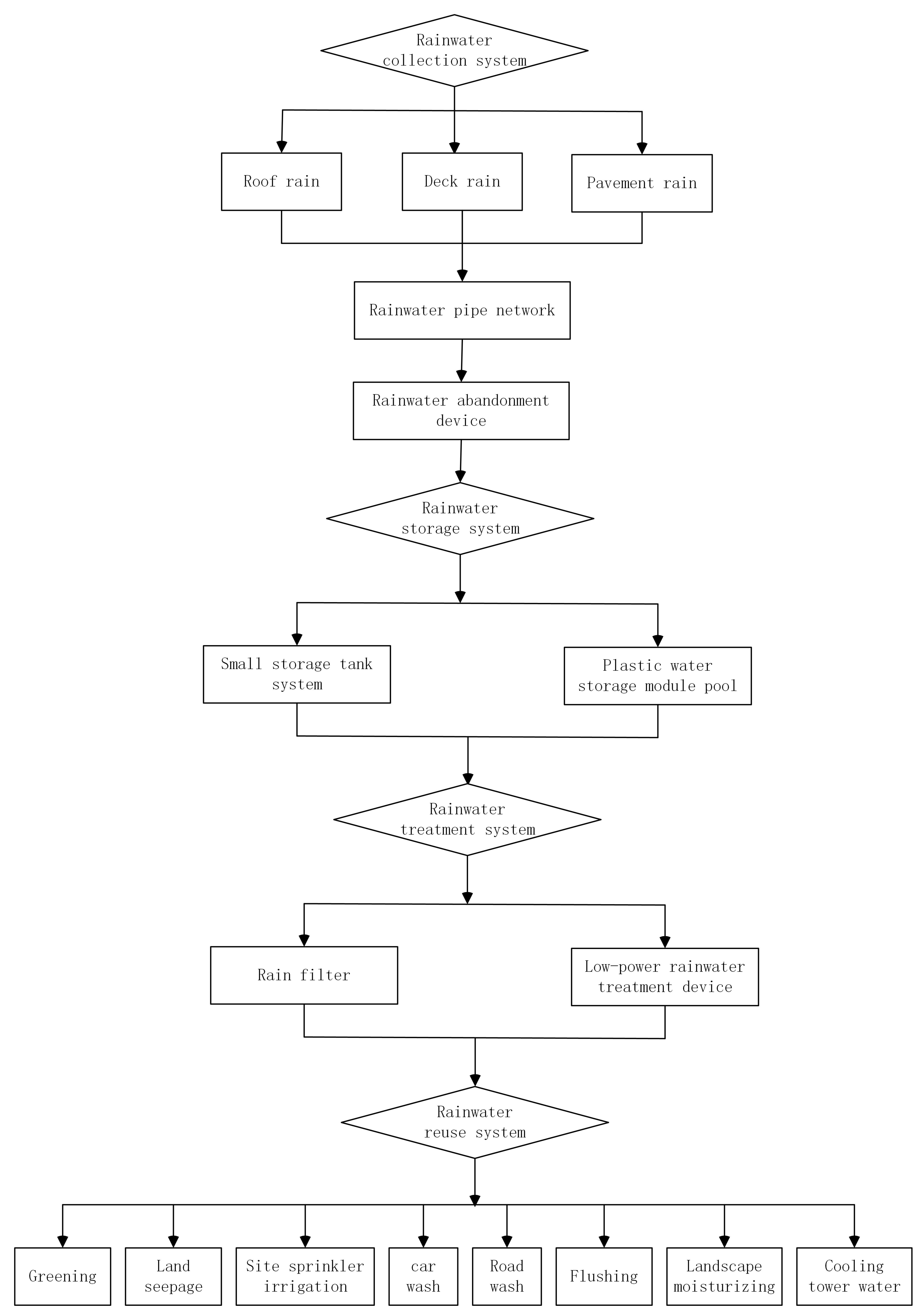
3.2. Ontology Mapping on Sponge City Rainwater Treatment System Ontologies
At the end of the last century, many developed countries have incorporated the concept of sponge cities in urban construction. In terms of sponge city construction technology, the United States first proposed the concept of low-impact development, and then scholars have conducted in-depth research on low-impact development and construction technology. During the development process, the United States also experienced water shortages such as urban water shortages and severe waterlogging during heavy rains. Subsequently, the United States began to study solutions to water resource problems. In the 1970s, the United States had proposed “best management measures”, and for the first time cited in the amendment of the Federal Water Pollution Control Act, which has gradually developed into a comprehensive and sustainable measure to control water quality and rainfall runoff (see Dietz [
33]). In 1999, the US Commission on Sustainable Development proposed the concept of green infrastructure, which simulates natural processes to accumulate, delay, infiltrate, transpiration, and reuse rainwater runoff to reduce urban load. The University of Portland conducted research on green roofs and found through actual tests that build a traditional roof into a green roof can intercept 60% of rainwater. Australia has proposed a toolkit for integrated urban water resource management software system. After its application in Sydney’s Botany area, the demand for municipal water supply has been reduced by 55%, achieving the comprehensive goals of water-saving, emission reduction and flood control, which has greatly improved Sydney’s water resources and environment. Several recent advances in sponge city can be referred to Li et al. [
34], Nguyen et al. [
35], McBean et al. [
36], Lashford et al. [
37], Gies [
38], Buragohain et al. [
39], Van Rooijen et al. [
40] and Wang et al. [
41].
The rainwater treatment system is the core of the sponge city technology. The working process of the new seepage rainwater well is that the rainwater in the community is collected through the cross slope, and the debris is filtered into the rainwater well through the grate. The rainwater entering the rainwater well passes through the perforated concrete floor of the hole, and the permeable geotextile and gravel layer complete the sediment filtration and then enter the permeable gravel well and penetrate into the benign permeable sand layer underground. The infiltration conditions of the new type of seepage rainwater well in sponge city are roughly divided into three types:
- (1)
The rainfall is very small. The rainwater well collects all the rainwater. The rainwater quickly infiltrates into the permeable sand layer through the permeable gravel well. The infiltration rainfall is the rainwater well.
- (2)
The rainfall is large. The rainwater collected by the rainwater well is accumulated in the well, but the water level does not reach the height of the overflow area, and the rainwater will also infiltrate into the permeable sand layer through the permeable gravel well, and the infiltration rainfall is the rainfall collected by the rainwater well.
- (3)
There is a lot of rainfall. The rainwater collected by the rainwater well is accumulated in the well. The water level exceeds the height of the overflow area. Part of the rainwater is drained through the overflow rainwater pipeline. The rainwater below the overflow area infiltrates into the permeable sand layer through the permeable gravel well. The infiltration rainfall is the rainfall infiltration into the sand layer below the height of the overflow area of the rainwater well. The infiltration rainfall, in this case, is the maximum infiltration rainfall of the new infiltration rainwater well.
By means of this background knowledge, we constructed four sub-ontologies for rainwater collection and treatment, and their basic structures can be shown in the following
Figure 2,
Figure 3,
Figure 4 and
Figure 5.
Our goal is to build ontology mapping among four ontologies, i.e., to find the most similar concepts from different ontologies. During the execution of this experiment, we chose nearly half of the vertices as sample points, and obtained the ontology function through the ontology learning algorithm in this paper, thus establishing a similarity-based ontology mapping. In order to explain the superiority of the algorithm in this paper, we also apply the ontology learning algorithms presented in articles [
11,
16,
17] to the sponge city rainwater treatment ontologies. The ontology sample sets are composed of 37 ontology vertices (denoted by
) and eight ontology vertices (denoted by
), respectively. Some comparison results are shown in
Table 3 and
Table 4.
It can be seen from the data manifested in
Table 3 and
Table 4 that the ontology learning algorithm in this paper is better than the other three types of ontology learning techniques, and its
accuracy is higher. This table above shows that the algorithm proposed in our paper is effective for sponge city rainwater treatment system ontologies.
4. Conclusions and Discussion
In this article, we present an ontology sparse vector learning algorithm based on a graph structure learning framework. The basic idea is to use a graph to represent the intrinsic relationship between the components of the ontology sparse vector, and obtain the calculation strategy through graph optimization. At the same time, we constructed two types of new ontologies in two different engineering fields, and applied the proposed ontology sparse vector learning trick to the new ontology to verify the feasibility of the method.
Structure learning is an important content of machine learning, and the structure of data can be represented by graphs in many frameworks, such as ontology graphs to represent ontology. On the other hand, in the process of digitizing the ontology, the information of each vertex needs to be encapsulated with a fixed-dimensional vector. What we consider is that some information in the encapsulated information is related to each other, and thus some components in the corresponding vector are related to each other. From this point of view, the focus of this article is to consider the internal structure of the ontology vector, express the optimization vector using a graph, and get the optimization algorithm by means of the knowledge of graph optimization and spectral graph theory. The main finding of this paper is that the algorithm obtained by learning the ontology vector from the internal structure of the vector is effective for some application fields.
For more technological details, the standard trick to deal with ontology optimization framework is gradient descent, the process of execution like this: compute the derivative and set it to zero, then solve the equation (group) and determine the parameters. However, in our paper, gradient descent cannot be directly used because
in Equation (
22) is not a differentiable function. It leads to absolute value function
is appeared in Equation (
25) which is also a non-differentiable function. This is why we need to introduce a soft-thresholding operator in Equation (
27) and then use iterative methods to obtain approximate solutions.
The existing researches reveal that although the value of the dimension p of the ontology vector is often very large in data representation, only a small part of the information plays a role when it comes to a specific application. A distinctive feature of ontology is that, for different engineering application backgrounds, the labels of ontology samples for supervised learning will be completely different. Furthermore, under the sparse vector framework, the optimal ontology sparse vector obtained is completely determined by the label of the ontology sample, in other words, it is completely determined by a specific application background.
This brings about a practical problem: for the labeled ontology sample vertex , corresponds to a fixed multi-dimensional vector (assuming that the ontology graph does not change during the entire learning process, and then each ontology vertex corresponds to the initial information representation the vector is fixed), but the value keeps changing with the application background. In other words, the determination of the value of is heavily dependent on domain experts. This awkward situation directly causes the entire ontology learning process to rely heavily on the participation of domain experts. In the absence of domain experts, it is impossible to provide a certain amount of information , making learning impossible or forced to transform into unsupervised learning.
It is gratifying that the technology of automatically generating samples has gradually matured in machine learning and has been applied to various fields of computer science, such as image processing, data analysis, and prediction. Therefore, combined with the characteristics of the ontology itself, it is necessary for us to introduce the automatic sample generation technology into the ontology learning based on sparse vectors, thereby reducing the dependence of ontology learning on domain experts in the future studying.
Another disadvantage of the algorithm in this paper can be described as follows. Since the ontology is a dynamic database, as time goes by, new related concepts are added to the ontology database. This makes it possible to change the graph structure of the entire ontology and the types of ontology concepts. In this case, the number and components of the ontology sparse vector will also change accordingly, that is, the graph will change significantly. The data obtained under the previous ontology graph structure may not have reference value for the changed ontology, i.e., graph needs to be reconstructed, and the experiment needs to be re-evaluated. However, this kind of defect is faced by all the ontology learning algorithms, not only appeared in the ontology learning algorithm in this paper. With the increase of concepts in the ontology library, such problems will inevitably appear.


