Abstract
We study in this paper the dynamics of molecules leading to the formation of nematic and smectic phases using a mobile 6-state Potts spin model with Monte Carlo simulation. Each Potts state represents a molecular orientation. We show that, with the choice of an appropriate microscopic Hamiltonian describing the interaction between individual molecules modeled by 6-state Potts spins, we obtain the structure of the smectic phase by cooling the molecules from the isotropic phase to low temperatures: molecules are ordered in independent equidistant layers. The isotropic-smectic phase transition is found to have a first-order character. The nematic phase is also obtained with the choice of another microscopic Hamiltonian. The isotropic-nematic phase transition is a second-order one. The real-time dynamics of the molecules leading to the liquid-crystal ordering in each case is shown by a video.
1. Introduction
Nematic and smectic phases have been the subject of intensive investigations since the discovery of liquid crystals (LC) [1,2]. Liquid crystals are often made of elongated organic rode-shaped molecules (called calamitic), or of discotic, i.e., disk-like, molecules. Thus, LC are generated by strong structural anisotropy objects. The way these constituents are arranged to form LC depends usually on the temperature, but, for some mesomorphic phases, it can also be a function of the concentration of the molecules in a solvent. The LC phases are often called mesophases which include four kinds of structures, according to the degrees of symmetry and the physical properties of LC with respect to their molecular arrangement: nematic, smectic, cholesteric, and columnar LC.
In this paper, we are interested in the smectic and nematic phases. We know that the nematic phase is the closest phase to the liquid phase and the most common. It has no long-range positional order but a global orientational order. As for the smectic phase, it is the phase which looks like the most to a crystalline solid and for which molecules are ordered in equidistant layers. It shows a long-range positional order (at least in one direction) and also an orientational order in each layer.
Let us recall some important works which have contributed in one way or another to the advance in the understanding of the LC. We show next what is new in our present work.
Most theoretical studies have used Frank’s free energy [3,4,5] which is a phenomenological macroscopic expression of different mechanisms governing the structure of a LC. Numerous models have been developed for modeling LC based on Frank’s free energy:
where is the director, , , and are the splay-constraint, twist, and bend–distortion constants, respectively. Other mean-field calculations including the works in Refs. [6,7] have been carried out to study both the structural and thermodynamic properties of free-standing smectic films for two cases of enhanced pair interactions in the bounding layers. However, the use of the Frank’s free energy and other mean-field approaches, though may be useful for obtaining some thermodynamic properties, cannot give precision on the question of criticality, as it is well-known from statistical physics [8,9] (for example, Ising, Heisenberg, and Potts spins give the same mean-field critical exponents).
On the computing works including Monte Carlo simulations and molecular dynamics, there has been a large number of investigations using various models. There has been early numerical simulations on the isotropic-nematic transition [10,11] as well as other works using artificial interactions of molecules-recipient wall [12,13] or approximate free energy [14] for this transition. In a pioneer work, Fabbri and Zanonni [11] considered the Lebwohl–Lasher model [10] of nematogens consisting of a system of particles placed at the sites of a cubic lattice and interacting with a pair potential , where is a positive constant, , for nearest neighbors particles i and j and is the angle between the axis of these two molecules. This model which is a Heisenberg spin model localized on on a lattice paved the way for many other simulations in the following 20 years. Let us mention a few important works concerning the nematics. In Refs. [15,16], Monte Carlo simulations have been performed with a generalized attractive-repulsive Gay–Berne interaction which is derived from the Lennard–Jones potential. In Ref. [17], the authors have determined the phase diagram for a lattice system of biaxial particles interacting with a second rank anisotropic potential using Monte Carlo simulations for a number of values of the molecular biaxiality. In Ref. [18], simulations have been performed on the Lebwohl–Lasher model with the introduction of an amount of spin disorder. We can mention the review by Wilson [19] on the molecular dynamics and the books edited by Pasini et al. [20,21], which reviewed all important computing works. In particular, the reader is referred to Ref. [22] for a review on the recent progress in the atomistic simulation and modeling of smectic liquid crystals. We should mention also a numerical work on the nematic transition using Brownian molecular dynamics [23] and a few Monte Carlo works with molecules localized on the lattice sites [24,25].
All the works mentioned above did not take into account the mobility of the molecules in the crystal; therefore, they did not show how dynamical ordering of an LC is formed from the liquid phase. In addition, no simulations have been done to study the isotropic-smectic and isotropic-nematic phase transition taking into account the mobility of the molecules at the transition, in spite of a large number of experimental investigations which will be mentioned below.
Consider a system of N molecules interacting with each others. Experimentally, we know that temperature variation can create different kinds of ordering in LC such as nematic and smectic phases. However, there is the absence of theoretical or numerical studies starting with such an assembly of interacting “mobile” molecules with a microscopic Hamiltonian of the Potts model. In particular, there is no investigation on the dynamics of how nematic and smectic orderings are dynamically reached from their respective isotropic phase when the temperature decreases.
The absence of studies using “mobile” molecules with a microscopic Hamiltonian motivates the study presented in this paper. Here, we use the mobile molecule model with appropriate interactions allowing for generating the nematic and smectic ordering. We choose the mobile Potts interaction between molecules for the clarity in the demonstration of the dynamics, but our method can be extended to other interaction models such as those between the Heisenberg or XY spins.
In this work, we study both the smectic and the nematic phase transition. We will first describe the model for the smectic case in Section 2 and then we show the results obtained by Monte Carlo (MC) simulations. The six-state Potts model is used to characterize six different spatial molecular orientations. Contrary to lattice models used so far in simulations, the molecules of the present model can move from one site to another on a cubic lattice. Only a percentage of the lattice is occupied by these molecules, and the empty sites allow the molecules to move as in a liquid at high T. As will be seen, we succeed in obtaining the smectic ordering, by following the motion of molecules with decreasing temperature. Section 3 is devoted to the isotropic-nematic phase transition. We present the model Hamiltonian and the MC results. With an appropriate choice of interactions between molecules, we succeed in obtaining the nematic phase by cooling the LC from the isotropic phase. Concluding remarks are given in Section 4.
2. The Smectic Phase
2.1. Model
The Hamiltonian used to model the smectic LC is given by
where denotes the pair of nearest neighbors (NN). is the spin–spin exchange interaction such as
where , , and taken as the unit of energy in the following. We also take the Boltzmann constant so that the temperature shown below is in the unit of .
The in-plane and inter-plane exchange interactions are then ferromagnetic and anti-ferromagnetic, respectively. The use of an antiferromagnetic between planes is to avoid a correlation between adjacent planes: the antiferromagnetic interaction favors different spin orientations between NN planes. The Potts spin has six values which represent six spatial molecular orientations. Note that these orientations can be arbitrary with respect to the lattice axes. For example, the six molecular orientations can be in the plane so that can take any angle among the six. They can be six orientations in a three-dimensional space where is described by two angles with , and . The Potts model does not need a specification of the value of the molecular orientation: if the NN orientations are similar, the energy is ; otherwise, the energy is zero.
2.2. Method of Simulation
The model used in this paper is based on a mobile Potts model with anisotropic interactions as seen earlier. An isotropic model has been used to study the melting of a crystal [26], not in the LC context.
We consider a system of molecules on a simple cubic lattice with sites. Each site i can thus be vacant or occupied at most by a molecule having orientations (). A molecule can thus move from one site to a neighboring empty site under the effects of the interaction with neighboring molecules at the temperature T. Obviously, the concentration of molecules must be lower than one to permit their motion.
We fix a concentration c low enough to allow the motion of molecules inside the recipient. The use of periodic boundary conditions in three directions reduces the size effect. We use several recipient volumes to test the validity of our results, and we see that results do not qualitatively change.
The simulation is carried out as follows: we generate the positions and the orientations of the molecules randomly in the recipient, we update each molecule position and orientation at the same time by using the Metropolis algorithm [27,28] applying to its old and trial new states. The position update is done by moving the molecule to a nearby vacant site with a probability for the simple cubic lattice. The motion of each molecule is therefore driven by just the interaction with its neighbors at a given temperature T. We start from a random configuration, namely from the disordered phase, and we slowly cool the system with an extremely small interval of T.
In simulations, we discard a large number of MC steps per molecule to equilibrate the system before averaging physical quantities over a large number of MC steps. We calculate in general the energy, the specific heat, an appropriate order parameter and its fluctuations (namely, susceptibility), the average coordination number, and the diffusion coefficient. For the smectic phase, the order parameter is the layer magnetization, which is defined for layer m by
where is the number of molecules present on layer m and where the sum is performed over all the spins belonging to the layer m. We see that, for an ordered system, there is only one kind of orientation in layer m so that , while, for a disordered system, there are q kinds of orientations equally present, namely with the same concentration , on layer m, so that . Here, we take molecular orientations.
The magnetic susceptibility is calculated by using thermal fluctuations of the order parameter : . During Monte Carlo steps at a given T, we average and . At the end of the simulation, we use the above formula to calculate . We have performed calculations for 300 temperatures between 0 and 5 by slow heating and slow cooling. The peak of indicates the transition temperature.
The diffusion coefficient is defined as
where is the averaging MC time duration, denotes the position of the molecule ℓ after moving, at time t, at temperature T, and that of the molecule before moving.
Due to the nature of the smectic ordering, we need to calculate separately the in-plane diffusion coefficient and the perpendicular one . The sum has to be performed for ℓ belonging to the plane and to the z direction, respectively.
We slowly cool the system from high temperatures, namely from the isotropic phase, taking in general 300 temperatures down to 0.
We record all physical quantities and the motion of molecules as the time evolves.
2.3. Results
Let us show in Figure 1 snapshots taken in the isotropic phase and in the final phase at with , with . As seen, the low-T phase is smectic with ordered planes but no correlation in the perpendicular direction.
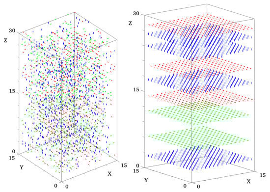
Figure 1.
Snapshot of the system at two different temperatures. Molecules are contained in a box with periodic boundary conditions. There is sites and 2025 molecules, i.e., a molecule concentration equal to . Each colored point corresponds to a molecular orientation. (Left): Initial configuration of the system at a high temperature . The system is completely disordered. (Right): Final configuration at low temperature . The system was cooled down from the disordered phase. Molecules are staged in independent layers and within a layer all molecules have the same orientation (same color). It corresponds to a smectic phase.
A video showing the dynamics of the formation of the smectic phase is available at the link given in Ref. [29].
The energy per molecule U is shown in Figure 2a versus T. We see clearly that there is a transition from the isotropic state to the smectic ordering at (in unit of ) where U changes the curvature. The parallel and perpendicular diffusion coefficients, and , are shown as functions of T in Figure 2b together with the total diffusion coefficient D. As seen, these curves change the curvature at the same transition temperature . Note that at any T means that the motion of molecules in the z direction is easier than in the plane. This is understood because of the densely ordered molecules in the plane in the smectic phase.
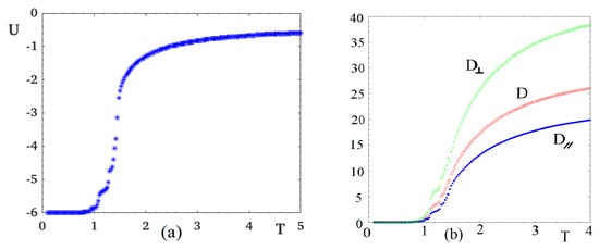
Figure 2.
(a) energy U versus T; (b) diffusion coefficients as functions of T: the upper curve (green) is the perpendicular diffusion coefficient, the lower curve (blue) is the parallel one and the middle curve (red) is the total diffusion coefficient. See text for comments. The molecule concentration c is , with . The exchange interactions are , , with .
Let us show in Figure 3 and dynamically in the video, Ref. [29], the histogram of the coordination number of the lattice sites in the smectic phase. As seen, most of them have 4 neighbors, indicating a planar or smectic phase phase. The antiferromagnetic interaction in the z-direction prevents two adjacent planes from having the same orientation.
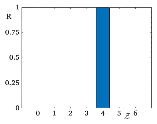
Figure 3.
Histogram showing the percentage R of sites having nearest neighbors at , i.e., corresponding to the snapshot at the right of Figure 1. Molecules are distributed such as they have mostly four neighbors, meaning they are staged in layers.
The order parameter of the smectic phase is the layer magnetization. Different layers have slightly different magnetizations, with more or less order, but they all show the transition at . Two typical layer magnetizations are shown in Figure 4 together with their susceptibilities.
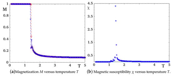
Figure 4.
Evolution of magnetizations of layer 3 (red) and 14 (blue) and their susceptibilities as functions of temperature. The molecule concentration c is , with . The exchange interactions are , .
At this stage, we emphasize that the transition from the isotropic to the smectic phase is of first order as observed by the sharp curvature changes in U and D and the vertical fall of the order parameter, at the transition. This is not surprising because the model considered here is equivalent to the 6-state Potts model and the phase transition we observe here takes place in each 2D plane. It is known from the Potts model that the transition of the q-state Potts model in 2D is of first order for [8].
Let us touch upon experimental observations on the nature of the smectic-isotropic phase transition. The determination of the nature of the phase transition in LC is not easy experimentally and theoretically. Unlike solid magnetic materials where the spin lattice models can be used efficiently to describe the phase transitions, molecules in LC often not only have structures that are too complicated, but also their spatial mobility, making it difficult to be represented by spin models. A transition in an LC often combines a disordering of molecular orientations and a rearrangement of their positions. There has therefore been a small number of such studies in the past. We can mention some important experimental works to show that the phase transition in LC is complex. Dogic has shown the role of the surface freezing in a two-step pathway of the isotropic-smectic phase transition in colloidal rods [30]. Dogic and Fraden [31] have also developed a model colloidal liquid crystals to study the kinetics of the isotropic-smectic transition. They have observed a number of novel metastable structures of unexpected complexity. They have also investigated the smectic phase in a colloidal suspension of semi-flexible virus particles [32] and found that a transition to the isotropic phase is of first order. Other complicated experimental observations have been reported [33,34,35,36]. On the theories, some works mostly based on the Landau theory have been carried out to show that, depending on the Hamiltonian, the isotropic-smectic transition is complicated, and can be of first or second order [37,38,39].
It should be noted that, for other ferromagnetic values of , we obtain the same results with a shift in the value of .
Other recipient sizes and values of interactions give the same qualitative results. The only constraint of the model is the in-plane interaction is ferromagnetic and the inter-plane one is antiferromagnetic.
3. The Nematic Phase
We study in this section two important points. The first point is how dynamically the molecules arrange themselves in a nematic phase when the system is cooled from the isotropic phase. The second point is the temperature dependence of physical quantities describing the nematic phase.
There has been a large number of paper since the 1970s on the theory of the nematic phase. As stated in the Introduction, all these works used the Landau–de Gennes mean-field approximation and the Frank’s free energy [40,41,42,43,44]. Let us briefly comment on a representative work. In Ref. [40], a review is given for the wide variety of predictions that results from a Landau-type of description of the nematic-isotropic phase transition. The various predictions are compared with the available experimental results. It is concluded that there is still no clear picture about the nature of the singularity near the nematic-isotropic phase transition. Though the assumption of classical (mean-field) critical behavior seems to be incorrect, there is no conclusive proof.
Experimental works on the isotropic-nematic transition were numerous. As in the smectic case, experimental systems are very different in nature, ranging from virus to macromolecules [45,46,47,48,49,50,51,52]. Let us comment some representative works. A detailed discussion was given in Ref. [45] on the weakly first-order character of the nematic-isotropic phase transition in liquid crystals observed in seven compounds. In Ref. [46], a report was made on a first-order isotropic-to-nematic phase transition induced by shear in concentrated solutions of elongated flexible worm-like micelles, using small-angle neutron scattering under shear. In Ref. [50], a quasi-elastic light scattering measurement of the isotropic-nematic phase transition of a liquid crystal in silica gel has been studied. It was found that the observation is consistent with a second-order phase transition.
The above-mentioned theoretical and experimental works, among others, do not give a firm conclusion on the nature of the isotropic-nematic phase transition. This motivates our work shown below. We find a second-order transition.
In the following, we introduce our microscopic Hamiltonian which gives rise to the formation of the nematic phase. We will next study physical quantities of this phase as functions of temperature.
3.1. Model
To model the nematic phase, we use also the mobile Potts model as above and, in Ref. [26], except that the interactions are given by the following Hamiltonian:
where the first two sums are performed over the nearest neighbors (NN) and the next-nearest neighbors (NNN), respectively. is the Kronecker delta and and denote the exchange interactions between molecules and are chosen such as the interactions between NN are antiferromagnetic (), and ferromagnetic for the NNN (). The last sum is performed over all the sites and corresponds to a slight anisotropy along the z-direction. To each state, is associated with a 3-components normalized vector . is then the z-component of the molecule .
We explain the choice of the above Hamiltonian which is guided by the following nematic phase: (i) there should not be molecules sticking to each other by mutual NN interaction, and the NN antiferromagnetic interaction is introduced to avoid the formation of ordered aggregates at low T; (ii) the NNN ferromagnetic interaction between further neighbors allows for a directional ordering observed in the nematic phase; and (iii) the small single-ion anisotropy is introduced to break the degeneracy of the three direction.
The method of simulation is shown above, and physical quantities are recorded with time evolution.
3.2. Results
A video showing the evolution of the nematic system with the time during a cooling can be viewed at Ref. [53].
We show in Figure 5 snapshots taken in the isotropic phase and in the final phase at with , where is chosen as the unit of energy. As in the smectic case, the temperature is in the unit of . At low-T, the nematic phase is found, and the molecules are oriented in the z-direction without positional ordering.
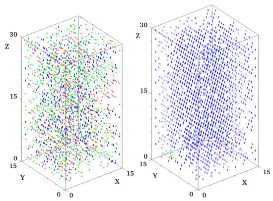
Figure 5.
Snapshot of the system at two different temperature. Molecules are contained in a box. There is sites and 2025 molecules, i.e., a molecule concentration equal to . Each colored point corresponds to a molecule orientation. (Left): Initial configuration of the system at high temperature (T is in unit of ). The system is completely disordered. (Right): Final configuration at low temperature obtained by a slow cooling. Note that that there is no positional order like for liquids. It corresponds to a nematic phase. A video showing the cooling of the system is available here.
The internal energy per molecule U and the diffusion coefficient D are shown in Figure 6. One observes that there is a transition from the isotropic phase to the nematic phase at , with the change of curvature of U and D.
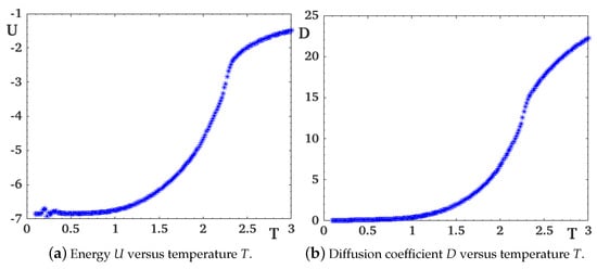
Figure 6.
Evolution of energy U and diffusion coefficient D versus T. The molecule concentration c is , with . The exchange interactions are , , with , and the anisotropy is equal to .
We show in Figure 7 the orientational order parameter which is in fact a sum of all molecules averaged with the time evolution. The susceptibility is also shown. These quantities confirm the sharp transition mentioned above.
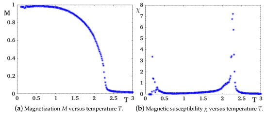
Figure 7.
Evolution of the orientational order parameter and its susceptibility as functions of T. The molecule concentration c is , with . The exchange interactions are , , and the anisotropy is equal to ().
The histogram of the coordination number is shown in Figure 8, where one sees that the quasi-totality of molecules have no NN as it should be in a nematic phase because it has no positional ordering.
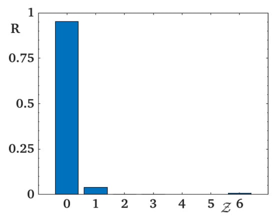
Figure 8.
Histogram showing the percentage R of sites having nearest neighbors at , i.e., corresponding to the snapshot on the right in Figure 5. Molecules have distributed such as they have no neighbors.
A video showing the dynamics of the system leading to the formation of the nematic phase is available here.
To close this section, we emphasize that the isotropic-nematic transition observed in our model shows a second-order character. We have seen above that experimental works have found both second- and first-order transitions. This is not surprising because experimental systems are so different in nature, ranging from virus to polymers, passing by complex chemical macromolecules. We know in the theory of phase transitions that the nature of the phase transition depends essentially on the symmetry of the order parameter and the nature of the microscopic molecular interaction. The molecular mobility adds another difficulty because of the melting/evaporation phenomenon at the crystal surface. Our nematic model can be applied to LC of rigid but mobile molecules with short-range interaction.
4. Conclusions
In this paper, we have shown that, by choosing appropriate interactions for the Hamiltonian of interacting 6-orientation mobile molecules, we can observe with time evolution how the nematic and smectic orderings are formed from the isotropic phase by decreasing the temperature.
For both systems, we have considered molecules moving in three-dimensional recipients with periodic boundary conditions in all directions. Various physical quantities, such as energy, order parameters, and diffusion coefficient, as functions of temperature have been calculated. Thus far, there have not been investigations using mobile molecules with a microscopic Hamiltonian.
For the smectic phase, it suffices to take a strong in-plane ferromagnetic interaction and an antiferromagnetic interaction in the z-direction. Upon cooling the system from the isotropic phase, the molecules gathered in independent equidistant planes thus constituting a smectic structure. The isotropic-smectic phase transition is found to be of first order. Note, however, that the order of the transition depends on the model chosen to represent the molecules. With the present Potts model, we find a first-order transition.
To simulate nematic phase, we have chosen antiferromagnetic interactions between the NN and a stronger ferromagnetic interaction between NNN. We have also added a slight anisotropy following the z-component of each spin. When cooling the system from the liquid phase, i.e., isotropic phase, molecules all have the same direction but no long-range positional ordering of any kind, namely no chains or planes. This is the nematic phase. The isotropic-nematic transition is found to be of second order for our model. Note that, in the theory of phase transitions and critical phenomena, phase transitions of the second order are classified into universality classes. Usually, phase transitions in different systems can belong to the same universality class characterized by a set of critical exponents. A university class depends on a small number of physical parameters such as the space dimension, the symmetry of the order parameter, and the nature of the interaction (short- or long-range, frustrated or not) as known from the renormalization group analysis. The nature of the phase transition does not depend on the value of the interaction. This value moves the critical temperature but does not change the universality class (see Ref. [9] for example, or any text book on Statistical Physics). There are well-known universality classes such as 2D Ising model, 3D Ising model, 3D XY spin model, 3D Heisenberg model, 2D Potts models, etc. Now, for first-order transitions, there are of course no divergences, but discontinuities at the transition of physical quantities (energy, order parameter, ⋯). A first-order transition is usually driven by competing interactions [54]. As seen in Section 2 and Section 3, experimental data show both second- and first-order transition for isotropic-smectic and isotropic-nematic transition. The determination of the order of the transition is very important in the theory of phase transitions. In experimental systems, there are so many kinds of molecules, and there cannot be a model for all nematics and a model for all smectics. This is why we have to choose a right spin model and an appropriate Hamiltonian to interpret a particular experiment.
Author Contributions
Conceptualization, A.B.-R. and H.T.D.; methodology, H.T.D.; software, A.B.-R.; formal analysis, A.B.-R.; writing the original draft preparation, A.B.-R.; writing review and editing, H.T.D. All authors have read and agreed to the published version of the manuscript.
Funding
This research received no external funding.
Conflicts of Interest
The authors declare no conflict of interest.
References
- de Gennes, P.G.; Prost, J. The Physics of Liquid Crystals, 2nd ed.; Oxford University Press: Oxford, UK, 1995. [Google Scholar]
- Liquid Crystals in Complex Geometries; Crawford, G.P., Zumer, S., Eds.; Taylor & Francis: London, UK, 1996. [Google Scholar]
- Gârlea, I.C.; Mulder, B.M. The Landau-de Gennes approach revisited: A minimal self-consistent microscopic theory for spatially inhomogeneous nematic liquid crystals. J. Chem. Phys. 2017, 147, 244505. [Google Scholar] [CrossRef] [PubMed]
- Chen, J.-H.; Lubensky, T.C. Landau-Ginzburg mean-field theory for the nematic to smectic-c and nematic to smectic-a phase transitions. Phys. Rev. A 1976, 14, 1202. [Google Scholar] [CrossRef]
- Chu, K.C.; McMillan, W.L. Unified Landau theory for the nematic, smectic a, and smectic c phases of liquid crystals. Phys. Rev. A 1977, 15, 1181. [Google Scholar] [CrossRef]
- Zakharov, A.V.; Sullivan, D.E. Transition entropy, Helmholtz free energy, and heat capacity of free-standing smectic films above the bulk smectic-A-isotropic transition temperature: A mean-field treatment. Phys. Rev. E 2010, 82, 041704. [Google Scholar] [CrossRef] [PubMed]
- Sliwa, I.; Zakharov, A.V. Structural, Optical and Dynamic Properties of Thin Smectic Films. Crystals 2020, 10, 321. [Google Scholar] [CrossRef]
- Baxter, R.J. Exactly Solved Models in Statistical Mechanics; Academic Press: New York, NY, USA, 1982. [Google Scholar]
- Diep, H.T. Statistical Physics—Fundamentals and Application to Condensed Matter; World Scientific: Singapore, 2015. [Google Scholar]
- Lebwohl, P.A.; Lasher, G. Nematic-Liquid-Crystal Order-A Monte Carlo Calculation. Phys. Rev. A 1972, 6, 426, Erratum in 1973, 7, 2222. [Google Scholar] [CrossRef]
- Fabbri, U.; Zannoni, C. A Monte Carlo investigation of the Lebwohl–Lasher lattice model in the vicinity of its orientational phase transition. Mol. Phys. 1986, 58, 763–788. [Google Scholar] [CrossRef]
- Xu, J.; Xu, J.; Selinger, R.L.; Selinger, J.V.; Shashidhar, R. Monte Carlo simulation of liquid-crystal alignment and chiral symmetry-breaking. J. Chem. Phys. 2001, 115, 4333–4338. [Google Scholar] [CrossRef]
- Binder, K.; Horbach, J.; Vink, R.; De Virgiliis, A. Confinement effects on phase behavior of soft matter systems. Soft Matter 2008, 4, 1555–1568. [Google Scholar] [CrossRef]
- Armas-Pérez, J.C.; Londono-Hurtado, A.; Guzmán, O.; Hernández-Ortiz, J.P.; de Pablo, J.J. Theoretically Informed Monte Carlo Simulation of Liquid Crystals by Sampling of Alignment-Tensor Fields. J. Chem. Phys. 2015, 143, 044107. [Google Scholar] [CrossRef]
- Berardi, R.; Zannoni, C. Do thermotropic biaxial nematics exist? A Monte Carlo study of biaxial Gay-Berne particles. J. Chem. Phys. 2000, 113, 5971–5979. [Google Scholar] [CrossRef]
- Berardi, R.; Fava, C.; Zannoni, C. A generalized Gay-Berne intermolecular potential for biaxial particles. Chem. Phys. Lett. 1995, 236, 462–468. [Google Scholar] [CrossRef]
- Biscarini, F.; Chiccoli, C.; Pasini, P.; Semeria, F.; Zannoni, C. Phase diagram and orientational order in a biaxial lattice model: A Monte Carlo study. Phys. Rev. Lett. 1995, 75, 1803. [Google Scholar] [CrossRef]
- Bellini, T.; Buscaglia, M.; Chiccoli, C.; Mantegazza, F.; Pasini, P.; Zannoni, C. Nematics with quenched disorder: What is left when long range order is disrupted? Phys. Rev. Lett. 2000, 85, 1008. [Google Scholar] [CrossRef]
- Wilson, M.R. Progress in computer simulations of liquid crystals. Int. Rev. Phys. Chem. 2005, 24, 421–455. [Google Scholar] [CrossRef]
- Pasini, P.; Zannoni, C.; Žumer, S. (Eds.) Computer Simulations of Liquid Crystals and Polymers: Proceedings of the NATO Advanced Research Workshop on Computational Methods for Polymers and Liquid Crystalline Polymers; Springer Science & Business Media: Berlin/Heidelberg, Germany, 2006; Volume 177. [Google Scholar]
- Pasini, P.; Zannoni, C. (Eds.) Advances in the Computer Simulatons of Liquid Crystals; Springer Science & Business Media: Berlin/Heidelberg, Germany, 2000; Volume 545. [Google Scholar]
- Glaser, M.A. Atomistic simulation and modeling of smectic liquid crystals. In Advances in the Computer Simulatons of Liquid Crystals; Springer Science & Business Media: Berlin/Heidelberg, Germany, 2000; Volume 545, p. 263. [Google Scholar]
- Repnik, R.; Ranjkesh, A.; Simonka, V.; Ambrozic, M.; Bradac, Z.; Kralj, S. Symmetry breaking in nematic liquid crystals: Analogy with cosmology and magnetism. J. Phys. Condensed Matter 2013, 25, 404201. [Google Scholar] [CrossRef]
- Ruhwandl, R.W.; Terentjev, E.M. Monte Carlo simulation of topological defects in the nematic liquid crystal matrix around a spherical colloid particle. Phys. Rev. E 1997, 56, 5561. [Google Scholar] [CrossRef]
- Gruhn, T.; Hess, S. Monte Carlo Simulation of the Director Field of a Nematic Liquid Crystal with Three Elastic Coefficients. Zeitschrift fu¨r Naturforschung A 1996, 51, 1–9. [Google Scholar] [CrossRef]
- Bailly-Reyre, A.; Diep, H.T.; Kaufman, M. Phase Transition and Surface Sublimation of a Mobile Potts Model. Phys. Rev. E 2015, 92, 042160. [Google Scholar] [CrossRef]
- Landau, D.P.; Binder, K. A Guide to Monte Carlo Simulations in Statistical Physics; Cambridge University Press: London, UK, 2009. [Google Scholar]
- Brooks, S.; Gelman, A.; Jones, G.L.; Meng, X.-L. Handbook of Markov Chain Monte Carlo; CRC Press: New York, NY, USA, 2011. [Google Scholar]
- Smectic Dynamics. Available online: https://youtu.be/aj6FVFCc4ig (accessed on 5 August 2020).
- Dogic, Z. Surface Freezing and a Two-Step Pathway of the Isotropic-Smectic Phase Transition in Colloidal Rods. Phys. Rev. Lett. 2003, 91, 165701. [Google Scholar] [CrossRef]
- Dogic, Z.; Fraden, S. Development of model colloidal liquid crystals and the kinetics of the isotropic-smectic transition. Phys. Eng. Sci. 2001, 359, 997–1015. [Google Scholar] [CrossRef]
- Dogic, Z.; Fraden, S. Smectic Phase in a Colloidal Suspension of Semiflexible Virus Particles. Phys. Rev. Lett. 1997, 78, 2417. [Google Scholar] [CrossRef]
- Coles, H.J.; Strazielle, C. Pretransitional Behaviour of the Direct Isotropic to Smectic a Phase Transition of Dodecylcyanobiphenyl (12CB). Mol. Cryst. Liq. Cryst. 1979, 49, 259–264. [Google Scholar] [CrossRef]
- Ocko, B.M.; Braslau, A.; Pershan, P.S.; Als-Nielsen, J.; Deutsch, M. Quantized layer growth at liquid-crystal surfaces. Phys. Rev. Lett. 1986, 57, 94, Erratum in 1986, 57,923. [Google Scholar] [CrossRef]
- Olbrich, M.; Brand, H.R.; Finkelmann, H.; Kawasaki, K. Fluctuations above the Smectic-A-Isotropic Transition in Liquid Crystalline Elastomers under External Stress. Europhys. Lett. 1995, 31, 281. [Google Scholar] [CrossRef]
- Jonsson, H.; Wallgren, E.; Hult, A.; Gedde, U.W. Kinetics of isotropic-smectic phase transition in liquid-crystalline polyethers. Macromolecules 1990, 23, 1041–1047. [Google Scholar] [CrossRef]
- Mukherjee, P.K.; Pleiner, H.; Brand, H.R. Simple Landau model of the smectic A-isotropic phase transition. Europ. Phys. J. E 2001, 4, 293–297. [Google Scholar] [CrossRef]
- Brand, H.R.; Mukherjee, P.K.; Pleiner, H. Mukherjee and Harald Pleiner, Macroscopic dynamics near the isotropic-smectic-A phase transition. Phys Rev. E 2000, 63, 061708. [Google Scholar]
- Mukherjee, P.K.; Pleiner, H.; Brand, H.R. Landau model of the smectic C-isotropic phase transition. J. Chem. Phys. 2002, 117, 7788. [Google Scholar] [CrossRef]
- Gramsbergen, E.F.; Longa, L.; de Jeu, W.H. Landau Theory of the Nematic-Isoropic Phase Transition. Phys. Rep. (Rev. Sect. Phys. Lett.) 1986, 135, 195–257. [Google Scholar]
- Sheng, P. Phase Transition in Surface-Aligned Nematic Films. Phys. Rev. Lett. 1976, 37, 1059. [Google Scholar] [CrossRef]
- Sheng, P. Boundary-layer phase transition in nematic liquid crystals. Phys. Rev. A 1982, 26, 1610. [Google Scholar] [CrossRef]
- Olmsted, P.D.; Goldbart, P.M. Isotropic-nematic transition in shear flow: State selection, coexistence, phase transitions, and critical behavior. Phys. Rev. A 1992, 46, 4966. [Google Scholar] [CrossRef] [PubMed]
- Fan, C.P.; Stephen, M.J. Isotropic-Namatic Phase Transition in Liquid Crystals. Phys. Rev. Lett. 1970, 25, 500. [Google Scholar] [CrossRef]
- Roie, B.V.; Leys, J.; Denolf, K.; Glorieux, C.; Pitsi, G.; Thoen, J. Weakly first-order character of the nematic-isotropic phase transition in liquid crystals. Phys. Rev. E 2005, 72, 041702. [Google Scholar] [CrossRef]
- Berret, J.-F.; Ron, D.C.; Porte, G.; Linder, P. Shear-Induced Isotropic-to-Nematic Phase Transition in Equilibrium Polymers. Europhys. Lett. 1994, 25, 521i–526i. [Google Scholar] [CrossRef]
- Tang, J.; Fraden, S. Magnetic-Field-Induced Isotropic-Namatic Phase Transition in a Colloiadal Suspension. Phys. Rev. Lett. 1993, 71, 3509. [Google Scholar] [CrossRef]
- Dogic, Z.; Purdy, K.R.; Grelet, E.; Adams, M.; Fraden, S. Isotropic-nematic phase transition in suspensions of filamentous virus and the neutral polymer Dextran. Phys. Rev. E 2004, 69, 051702. [Google Scholar] [CrossRef]
- Stinson, T.W., III; Litster, J.D. Pretransitional Phenomena in Isotropic Phase of a Nematic Liquid Crystal. Phys. Rev. Lett. 1970, 25, 503. [Google Scholar] [CrossRef]
- Wu, X.; Goldburg, W.I.; Liu, M.X.; Xue, J.Z. Slow Dynamics of Isotropic-Nematic Phase Transition in Silica Gels. Phys. Rev. Lett. 1992, 69, 470. [Google Scholar] [CrossRef]
- Germano, S. Iannacchione and Daniele Finotello, Calorimetric Study of Phase Transitions in Confined Liquid Crystals. Phys. Rev. Lett. 1992, 69, 2094. [Google Scholar]
- Dong, X.M.; Kimura, T.; Revol, J.F.; Gray, D.G. Effects of Ionic Strength on the Isotropic-Chiral Nematic Phase Transition of Suspensions of Cellulose Crystallites. Langmuir 1996, 12, 2076–2082. [Google Scholar] [CrossRef]
- Nematic Dynamics. Available online: https://youtu.be/WVd1t3XJxiQ (accessed on 5 August 2020).
- Diep, H.T. (Ed.) Frustrated Spin Systems; World Scientific: Singapore, 2013. [Google Scholar]
© 2020 by the authors. Licensee MDPI, Basel, Switzerland. This article is an open access article distributed under the terms and conditions of the Creative Commons Attribution (CC BY) license (http://creativecommons.org/licenses/by/4.0/).