Fuzzy Model Identification Using Monolithic and Structured Approaches in Decision Problems with Partially Incomplete Data

Abstract

A significant challenge in the current trend in decision-making methods is the problem’s class in which the decision-maker makes decisions based on partially incomplete data. Classic methods of multicriteria decision analysis are used to analyze alternatives described by using numerical values. At the same time, fuzzy set modifications are usually used to include uncertain data in the decision-making process. However, data incompleteness is something else. In this paper, we show two approaches to identify fuzzy models with partially incomplete data. The monolithic approach assumes creating one model that requires many queries to the expert. In the structured approach, the problem is decomposed into several interrelated models. The main aim of the work is to compare their accuracy empirically and to determine the sensitivity of the obtained model to the used criteria. For this purpose, a study case will be presented. In order to compare the proposed approaches and analyze the significance of the decision criteria, we use two ranking similarity coefficients, i.e., symmetric $r_w$ and asymmetric $WS$. In this work, the limitations of each approach are presented, and the results show great similarity despite the use of two structurally different approaches. Finally, we show an example of calculations performed for alternatives with partially incomplete data.

1. Introduction

Decision support methods are a significant branch of operational research. They are designed to support decision-making processes concerning an extensive range of problems. However, the main objective is to analyze complex decision-making processes, which very often requires the engagement of domain experts. The main challenge is also the analysis of many often conflicting decision criteria [1,2]. In those cases, multicriteria decision analysis (MCDA) methods are used to help the decision-maker to the right solution. However, there is another challenge with choosing the proper MCDA method because it is a problematic task [3,4]: Not every method will be able to handle uncertain or partially incomplete data [5]. Another problem is that most MCDA methods require knowledge of the importance of criteria weighting [6].

Before further discussion, let us recognize the difference between uncertainty and incompleteness. The cause of the uncertainty is the noise joined with the original value with a particular distribution. Experts apply different methods, e.g., interval number [7], fuzzy numbers [8,9], or gray numbers [10], to perform a calculation based on uncertain data. Incompleteness, on the other hand, is a lack of data. If a single criterion is missing, we need to consider all theoretically possible values from the domain. Moreover, with no additional information about the variable, it is a requirement [11].

There are currently many valuable MCDA methods that use certain data [12], and this includes methods such as Technique for Order of Preference by Similarity to Ideal Solution (TOPSIS) [13], Preference Ranking Organization Method for Enrichment Evaluations (PROMETHEE) [14], PROSA [15], the Analytic Hierarchy Process (AHP) [16,17], the Analytic Network Process (ANP) [18,19], VIKOR [20], ELECTRE [21], COmplex PRoportional ASsessment (COPRAS) [22,23], and many others [24]. These methods have certain limitations and are not suitable for resolving decision-making problems for uncertain or partially incomplete data. Therefore, many extensions have been and continue to be made. For example, we can list techniques, modifications, and improvements which allow solving more and more complex problems efficiently such as Fuzzy TOPSIS [25,26], fuzzy COPRAS [27,28], NEAT F-PROMETHEE [29,30], fAHP [31], Generalized PROSA [32], and many more [33,34,35]. Most of the extensions focus on calculations only on uncertain or incomplete data. However, the most rational approach seems to be to use methods that allow crisp or uncertain data at the same time.

The Characteristic Objects METhod (COMET) is a new MCDA developed [36] which uses an entirely different approach to solving decision problems [37]. It is based on the idea of characteristic objects, which are not strictly connected to alternatives. This makes it the first MCDA method that is entirely free of the rank reversal paradox [38]. An expert or detailed data analysis determines the number and characteristic values. Thus, there is no strict relationship between alternative values and characteristic objects. Therefore, changing the initial set of alternatives, either adding or subtracting a certain number of decision options, does not change the existing order of the elements in the set [39]. In this way, we get the original measuring system for the specific case. However, we must pay attention to the dimensional curse, which makes it challenging to use the COMET method effectively for problems with increased dimensional accuracy [40]. Two different approaches emerge for this purpose: One of them assumes tedious filling in the $MEJ$ decision matrix (monolithic approach), and the other one uses hierarchical decomposition of the problem (structured approach). The main problem is that it has not been empirically investigated how much difference we will make using both approaches.

In this paper, we present a study case in which we want to show a difference between structured and monolith approaches to solving MCDA problems using the COMET method. The example will be taken from the literature where two different methods were used to calculate the rankings of electric vans [41]. The PROMETHEE method was used for calculations of alternatives with certain data and the fuzzy TOPSIS method for decision variants with partially incomplete data. In our work, we identify the fuzzy model using a monolithic and structured approach, and then compare the results with the original ones in terms of the ranking obtained. For this purpose, two measures of similarity will be used: a symmetrical $r_w$ and an asymmetrical $WS$ coefficient. Both coefficients take into account that errors in the ranking at the top are more significant than at the end of the ranking. Another element of our contribution is the way of ranking the relevance of the criteria using a monolithic approach in the COMET method. Examination of the criteria’s significance is one of the fundamental challenges in decision-making. The analysis of the relevance of the criteria will also allow determining whether it is possible to reduce the decision-making model in order to avoid criteria with incomplete data. Finally, we show how to use the COMET method to get uncertain preference by using partially incomplete data.

The rest of the paper is structured as follows. Section 2 contains a description of the fuzzy set theory, the COMET method, and some coefficients which are used in our analyses. Section 3 describes the empirical study case. Results and discussion are presented in Section 4. The final summary and conclusions are contained in Section 5.

2. Preliminaries

2.1. Fuzzy Set Theory

The idea of Fuzzy Set Theory was introduced by Lofti Zadeh in [42]. Fuzzy Set Theory is used in many scientific fields and could be especially useful for solving MCDA problems [43,44,45]. Here, we present some definitions and basic concepts of the Fuzzy Set Theory which are necessary to understand COMET method [46,47].

Definition 1.

The fuzzy set A in a certain non-empty space of solutions X is defined by (1),

$$A=\left\{\left(x,{\mu }_A\left(x\right)\right);x\in X\right\},$$

(1)

where

$${\mu }_A\left(x\right):X\to [0,1],$$

(2)

is a membership function of the fuzzy set A. This function indicates the degree of the membership of the element in the set A. ${\mu }_A\left(x\right)=1$ means full membership, $0<{\mu }_A\left(x\right)<1$ means partial membership, and ${\mu }_A\left(x\right)=0$ means no membership at all.

Definition 2.

The triangular fuzzy number $A(a,m,b)$ is a fuzzy set whose membership function is defined as (3), and it is visualized in Figure 1.

$${\mu }_A(x,a,m,b)=\left\{\begin{array}{cc}0\hfill & x\le a\hfill \\ \frac{x-a}{m-a}\hfill & a\le x\le m\hfill \\ 1\hfill & x=m\hfill \\ \frac{b-x}{b-m}\hfill & m\le x\le b\hfill \\ 0\hfill & x\ge b\hfill \end{array}\right.$$

(3)

and fulfill characteristics (4) and (5):

$$x_1,x_2\in [a,m]\wedge x_2>x_1\Rightarrow {\mu }_A\left(x_2\right)>{\mu }_A\left(x_1\right)$$

(4)

$$x_1,x_2\in [m,b]\wedge x_2>x_1\Rightarrow {\mu }_A\left(x_2\right)<{\mu }_A\left(x_1\right)$$

(5)

Definition 3.

The support of a TFN—subset of the A set in which all elements have a non-zero membership value in the A set (6).

$$S\left(\tilde{A}\right)=x:{\mu }_{\tilde{A}}\left(x\right)>0=[a,b]$$

(6)

Definition 4.

The core of a TFN is a one-element fuzzy set (singleton) with membership value 1 (7).

$$C\left(\tilde{A}\right)=x:{\mu }_{\overline{A}}\left(x\right)=1=m$$

(7)

Definition 5.

The fuzzy rule—it is based on the Modus Ponens tautology. The IF-THEN, $OR$, and $AND$ logical connectives are used in the reasoning process.

Definition 6.

The rule base—it includes logical rules defining the relations in the system between the input and output sets.

Definition 7.

The intersection operator (T-norm)—it is a function modeling the $AND$ operation on some fuzzy numbers. This operator is described by using properties: boundary (8), monotonicity (9), commutativity (10), and associativity (11), for any $a,b,c,d\in [0,1].$

$$T(0,0)=0,T(a,1)=T(1,a)=a$$

(8)

$$T(a,b)<T(c,d)\iff ifa<candb<d$$

(9)

$$T(a,b)=T(b,a)$$

(10)

$$T(a,T(b,c\left)\right)=T\left(T\right(a,b),c)$$

(11)

Definition 8.

The S-norm operator or T-conorm is a function modeling the OR operator of two or more fuzzy numbers. It should fulfill the following properties; boundary (12), monotonicity (13), commutativity (14), and associativity (15), for any $a,b,c,d\in [0,1].$

$$S(1,1)=1,S(a,0)=S(0,a)=a$$

(12)

$$S(a,b)<S(c,d)\iff ifa<candb<d$$

(13)

$$S(a,b)=S(b,a)$$

(14)

$$S(a,S(b,c\left)\right)=S\left(S\right(a,b),c)$$

(15)

2.2. The COMET Method

The Characteristic Objects METhod (COMET) is based on fuzzy logic and triangular fuzzy sets. The accuracy of the COMET method was verified in previous works [48,49,50]. The formal notation of the COMET must be recalled based on the work in [36], and Figure 2 presents the flowchart of the COMET method as a summary.

Step 0. Initiate the process—it is a preparatory stage, which aims to identify the problem to be further analyzed clearly. In the beginning, it is necessary to define the purpose of the research and determine the specificity of the MCDA problem. Then, we should select an expert or a group of experts whose task will be to select decision alternatives and criteria for their evaluation. After selecting a group of alternatives, a set of criteria that should be taken into account in further analysis should also be selected.

Step 1. Definition of the space of the problem—the dimensionality of the problem is determined by the expert, which selects r criteria, $C_1,C_2,\dots ,C_r$. For each criterion $C_i$, e.g., $\{{\tilde{C}}_{i1},{\tilde{C}}_{i2},\dots ,{\tilde{C}}_{i{c}_i}\}$ (16) a set of fuzzy numbers is carefully selected:

$$\begin{array}{c}{C}_1=\left\{{\tilde{C}}_{11},{\tilde{C}}_{12},\dots ,{\tilde{C}}_{1c_1}\right\}\\ C_2=\left\{{\tilde{C}}_{21},{\tilde{C}}_{22},\dots ,{\tilde{C}}_{2c_2}\right\}\\ \cdots \\ C_r=\left\{{\tilde{C}}_{r1},{\tilde{C}}_{r2},\dots ,{\tilde{C}}_{r{c}_r}\right\}\end{array}$$

(16)

where $C_1,C_2,\dots ,C_r$ are the ordinals of the fuzzy numbers for all criteria.

Step 2. Generation of the characteristic objects—the characteristic objects ($CO$) are obtained with the usage of the Cartesian product of the fuzzy numbers’ cores of all the criteria (17):

$$CO=\langle C\left(C_1\right)\times C\left(C_2\right)\times \cdots \times C\left(C_r\right)\rangle$$

(17)

As a result, an ordered set of all $CO$ is obtained (18):

$$\begin{array}{c}C{O}_1=\langle C\left({\tilde{C}}_{11}\right),C\left({\tilde{C}}_{21}\right),\dots ,C\left({\tilde{C}}_{r1}\right)\rangle \\ C{O}_2=\langle C\left({\tilde{C}}_{11}\right),C\left({\tilde{C}}_{21}\right),\dots ,C\left({\tilde{C}}_{r1}\right)\rangle \\ \cdots \\ C{O}_t=\langle C\left({\tilde{C}}_{1c_1}\right),C\left({\tilde{C}}_{2c_2}\right),\dots ,C\left({\tilde{C}}_{r{c}_r}\right)\rangle \end{array}$$

(18)

where t is the count of $CO$s and is equal to (19):

$$t=\prod _{i=1}^r{c}_i$$

(19)

Step 3. Evaluation of the characteristic objects—the Matrix of Expert Judgment ($MEJ$) is determined by the expert, which comparing the $CO$s pairwise. The MEJ matrix is presented as follows (20),

$$MEJ=\left(\begin{array}{cccc}{\alpha }_{11}& {\alpha }_{12}& \cdots & {\alpha }_{1t}\\ {\alpha }_{21}& {\alpha }_{22}& \cdots & {\alpha }_{2t}\\ \cdots & \cdots & \cdots & \cdots \\ {\alpha }_{t1}& {\alpha }_{t2}& \cdots & {\alpha }_{tt}\end{array}\right)$$

(20)

where ${\alpha }_{ij}$ is the effect of comparing $C{O}_i$ and $C{O}_j$ by the expert. The function $f_{exp}$ express the individual judgment function of the expert. It is a representation of the knowledge of the selected expert, whose preferences can be presented as (21)

$${\alpha }_{ij}=\left\{\begin{array}{c}0.0,f_{exp}\left(C{O}_i\right)<f_{exp}\left(C{O}_j\right)\hfill \\ 0.5,f_{exp}\left(C{O}_i\right)=f_{exp}\left(C{O}_j\right)\hfill \\ 1.0,f_{exp}\left(C{O}_i\right)>f_{exp}\left(C{O}_j\right)\hfill \end{array}\right.$$

(21)

After the MEJ matrix is prepared, a vertical vector of the Summed Judgments ($SJ$) is obtained as follows, (22):

$$S{J}_i=\sum _{j=1}^t{\alpha }_{ij}$$

(22)

Finally, the values of preference are estimated for each characteristic object, and a vertical vector P is obtained. The i-$th$ row includes the estimated value of preference for $C{O}_i$.

Step 4. The rule base—each characteristic object and its value of preference is converted to a fuzzy rule as (23)

$$IFC\left({\tilde{C}}_{1i}\right)ANDC\left({\tilde{C}}_{2i}\right)AND\dots THEN{P}_i$$

(23)

In this way, a complete fuzzy rule base is obtained.

Step 5. Inference and the final ranking—each alternative is represented as a set of values, e.g., $A_i=\{{\alpha }_{i1},{\alpha }_{i2},{\alpha }_{ri}\}$. This set is addressed to the criteria $C_1,C_2,\dots ,C_r$. Mamdani’s fuzzy inference technique is used to calculate the preference of the i-$th$ decision variant. The constant rule base guarantees that the determined results are unequivocal, and it makes the COMET completely rank reversal-free.

2.3. Correlation Coefficients

Correlation coefficients make it possible to compare obtained results and determine how similar they are. In this paper we would use the sample Pearson correlation coefficient (24), the weighted Spearman correlation coefficient (25), and the rank similarity coefficient (26) to determine how similar obtained with COMET rankings to reference rankings.

2.3.1. The Sample Pearson Correlation Coefficient

The Pearson correlation coefficient is the ratio between the covariance of the two variables and the product of their standard deviations. The range value of the correlation coefficient is an interval from −1.0 to 1.0. The value of 1.0 means that we have a linear relationship which describes the relation between X and Y, with all data points lying on the line for which Y increases with X. The coefficient value of −1.0 means that all data points are on the line for which value of Y-variable decreases with increasing value of X-variable. A value of 0.0 means that there is no relationship between the variables. The Pearson correlation ratio, when applied to the sample data, is commonly represented by

$$r_{xy}=\frac{N\sum x_i{y}_i-\sum x_i\sum y_i}{\sqrt{N\sum x_i^2-{\left(\sum x_i\right)}^2}\sqrt{N\sum y_i^2-{\left(\sum y_i\right)}^2}}$$

(24)

N is sample size, $x_i$ and $y_i$ are the individual sample elements indexed with i, and $\overline{x}$ is the sample mean (analogously for $\overline{y}$).

2.3.2. Weighted Spearman’s Rank Correlation Coefficient

For a samples of size N, the rank values $x_i$ and $y_i$ are defined as (25). In this approach, the positions at the top of both rankings are more important. The weight of significance is calculated for each comparison. It is the element that determines the main difference to the Spearman’s rank correlation coefficient which examines whether the differences appeared and not where they appeared.

$$r_w=1-\frac{6{\sum }_{i=1}^N{(x_i-y_i)}^2((N-x_i+1)+(N-y_i+1))}{N^4+N^3-N^2-N}$$

(25)

2.3.3. Rank Similarity Coefficient

For a samples of size N, the rank values $x_i$ and $y_i$ are defined as (26) [51]. It is an asymmetric measure. The weight of a given comparison is determined based on the significance of the position in the first ranking, which is used as a reference ranking during the calculation.

$$WS=1-\sum _{i=1}^N{2}^{-x_i}\frac{|x_i-y_i|}{max\left(\right|x_i-1|,|x_i-N\left|\right)}$$

(26)

3. Empirical Study Case

3.1. Material

This study case is based on data and initial results published in [41], where Wątróbski et al. provide a hybrid MCDA approach as support for choosing electrical cargo vans for city logistic. They use the PROMETHEE II to rank vans with complete information and the fuzzy TOPSIS method to rank ones with gaps in data. In this paper, we present a comparison of two approaches using COMET method, i.e., monolithic and structured approaches. Both techniques allow dealing with both crisp and uncertain data and are resistant to the rank reversal phenomenon.

In the first step, we show two different models obtained by using the COMET method to calculate preferences for ten electric vans with complete data. The obtained results are compared with the initial results [41], and in this way the accuracy of both identified models will be validated. Selected alternatives will be evaluated from the perspective of criteria described in

Table 1. Description of the criteria.

Group of Criteria	${\mathit{C}}_{\mathit{i}}$	Criterion Name	Units	Direction
$P_1$ Performance	$C_1$	Carrying capacity	[kg]	max
	$C_2$	Max velocity	[km/h]	max
	$C_3$	Travel range	[km]	max
$P_2$ Engine	$C_4$	Engine power	[kW]	max
	$C_5$	Engine torque	[Nm]	max
$P_3$ Battery	$C_6$	Battery charging time 100%	[h]	min
	$C_7$	Battery charging time 80%	[min]	min
	$C_8$	Battery capacity	[kWh]	max
Price	$C_9$	Price	[thous. USD]	min

, where nine criteria are split into four groups.

In order to validate the correctness of the results, we use a group of ten alternatives according to the work in [41]. All decision variants have complete values for all attributes and are shown in

Table 2. Alternatives description.

${\mathit{A}}_{\mathit{i}}$	Name	${\mathit{C}}_1$	${\mathit{C}}_2$	${\mathit{C}}_3$	${\mathit{C}}_4$	${\mathit{C}}_5$	${\mathit{C}}_6$	${\mathit{C}}_7$	${\mathit{C}}_8$	${\mathit{C}}_9$
$A_1$	EVI MD	3000	96	145	200	610	10.0	120	99.0	120.0
$A_2$	EVI Walk-In Van	2000	100	145	200	610	10.0	120	99.0	90.0
$A_3$	e-NV200+	705	120	170	80	270	4.0	30	24.0	25.0
$A_4$	e-Wolf Omega 0.7	613	140	180	140	400	8.0	40	24.2	50.0
$A_5$	Minicab-MiEV Truck	350	100	110	30	196	4.5	15	10.5	12.9
$A_6$	Mitsubishi Minicab-MiEV (10.5 kWh)	350	100	100	30	196	4.5	15	10.5	15.5
$A_7$	Mitsubishi Minicab-MiEV (16 kWh)	350	100	150	30	196	7.0	35	16.0	18.7
$A_8$	Partner Panel Van	635	110	170	49	200	8.0	35	22.5	31.5
$A_9$	Phoenix Motorcars SUV	340	150	160	110	500	6.0	10	35.0	45.0
$A_{10}$	Piaggio Porter electric-power	750	57	110	10	80	8.0	120	35.0	24.4

.

Based on the selected group of alternatives, the corresponding characteristic values are indicated. Three values are indicated for each alternative, and a complete set of all characteristic values is presented in

Table 3. Description of the characteristic values.

${\mathit{C}}_{\mathit{i}}$	Name	Min	Mean	Max
$C_1$	Carrying capacity	340	909.3	3000
$C_2$	Max velocity	57	107.3	150
$C_3$	Travel range	100	144	180
$C_4$	Engine power	10	87.9	200
$C_5$	Engine torque	80	325.8	610
$C_6$	Battery charging time 100%	4	7	10
$C_7$	Battery charging time 80%	10	54	120
$C_8$	Battery capacity	10.5	37.57	99
$C_9$	Price	12.9	43.3	120

. The domain range of the problem state has been identified as the minimum and maximum values. The third characteristic value is indicated by using the adaptive approach as the arithmetic mean. This approach is dictated by the lack of an appropriate field expert. However, based on the data provided in the source paper and stochastic optimization methods, it is possible to fill in the MEJ matrix in a structured and monolithic approach.

The next step is to determine the triangular fuzzy numbers (TFNs), which are essential in the COMET method. Based on the characteristic values, 36 TFNs were obtained. They determine the definitions of the three linguistic values for each criterion, which are the low, medium, and high values of the attribute. They are presented in Figure 3.

3.2. Methods

The structured approach will use the hierarchy according to the classification from Table 1, and is presented in Figure 4. The monolithic model assumes the use of only one COMET block with nine criteria inputs.

The $P_1$ model describes the performance of the evaluated vehicles taking into account three-component criteria ($C_1$–$C_3$) [52,53,54]. When identifying it, 27 characteristic objects are created, which requires 351 queries to the expert, and the full MEJ matrix is shown in Figure 5 (left). When evaluating the engine (model $P_2$), only its power and torque are taken into account [53,55,56]. We get nine characteristic objects, and the MEJ matrix requires only 36 queries to the decision-maker, which are presented in Figure 5 (center). The battery evaluation modules ($P_3$) have the same complexity as the $P_1$ model and the MEJ matrix for this model is presented in Figure 5 (right) [56,57,58]. The last model in the structured approach is the P final model, which has four inputs, which are performance, engine, battery, and $C_9$ criterion [53,58], which is the vehicle price. At the same time, it is the largest of the models requiring 4095 comparisons of objects characteristic of the expert. This MEJ matrix is shown in Figure 6. In total, the concept of the structured approach requires 4833 pairwise comparisons. This is an approach which corresponds to a large reduction of comparisons compared to the monolithic approach. In the second case, only one model is created, which has nine inputs. This means that the number of characteristic objects is equal to $3^9$ because three characteristic values describe each criterion. This is related to the dimensional curse as such a reference would require more than 193 million pairwise comparisons. It is a number practically unattainable by humans because it would require the $MEJ$ matrix to be completed for more than six years (assuming one comparison per second). In order to complete the $MEJ$ matrix, we use the identification of characteristic dominated objects, stochastic optimization methods [39,59,60], and transitive relation of pairwise comparisons (27):

$${\forall }_{p,q,r\in X}p\prec q\wedge q\prec r\Rightarrow p\prec r$$

(27)

4. Results and Discussion

4.1. Comparison of the Monolithic and Structured Approaches

The decision models obtained, although they concern the same issue, have different numerical scales. The values obtained by using the structured approach, in addition to the final preferences, contain additional information on partial preferences for the evaluation of the performance, engine, and batteries of the considered freight vehicles, and the results are presented in the

Table 4. The obtained preference values for structured model.

${\mathit{A}}_{\mathit{i}}$	${\mathit{P}}_1$	${\mathit{P}}_2$	${\mathit{P}}_3$	${\mathit{P}}_{\mathit{struct}}$
$A_1$	0.7851	0.3684	1.0000	0.5732
$A_2$	0.6136	0.3684	1.0000	0.5972
$A_3$	0.5950	0.7151	0.3492	0.7718
$A_4$	0.7187	0.3927	0.6850	0.6996
$A_5$	0.1378	0.6439	0.1715	0.4911
$A_6$	0.0917	0.6439	0.1715	0.4619
$A_7$	0.3298	0.4342	0.1715	0.4595
$A_8$	0.5354	0.4062	0.2110	0.5138
$A_9$	0.6491	0.6901	0.6709	0.8374
$A_{10}$	0.0824	0.1496	0.0000	0.1512

.

An important issue is to know which of the analyzed approaches is more accurate. It may seem that the monolithic model could give more accurate results, but this way needs more pairwise comparisons than the structured approach. Moreover, creating intermediate models provides us with more information about the modeled decision problem. However, a large number of comparisons can influence the accuracy negatively.

Table 5. Preference values and rankings for structured and monolithic approaches, where $Ref$ means a place in the reference ranking from [41]; $P_{str}$ and $P_{mon}$ are preference values for the structured and monolithic approaches, respectively; and r(·) means ranking.

Alt	Ref	${\mathit{P}}_{\mathit{str}}$	$\mathit{r}\left({\mathit{P}}_{\mathit{str}}\right)$	${\mathit{P}}_{\mathit{mon}}$	$\mathit{r}\left({\mathit{P}}_{\mathit{mon}}\right)$
$A_1$	5	0.5732	5	0.5974	4
$A_2$	4	0.5972	4	0.5913	5
$A_3$	2	0.7718	2	0.6643	2
$A_4$	3	0.6996	3	0.6410	3
$A_5$	7	0.4911	7	0.4019	7
$A_6$	9	0.4619	8	0.3774	8
$A_7$	8	0.4595	9	0.3647	9
$A_8$	6	0.5138	6	0.4321	6
$A_9$	1	0.8374	1	0.7379	1
$A_{10}$	10	0.1512	10	0.0835	10

provides a complete list of reference values, obtained preferences, and rankings. The obtained preference results differ, which is natural with two different operational approaches. It should be noted, however, that the final ranking match is at a very high level. In the case of the monolithic approach, there have been two order replacements between the alternatives $(A_1,A_2)$ and $(A_6,A_7)$. Besides, in the case of structured approach it was only one pair $(A_1,A_2)$. In both of these cases, we have quite small differences in the value of preferences, and at the same time the correlation of preferences results in both models are highly correlated with each other and amount to 0.9756, which indicates an almost linear relationship.

However, the values of preferences alone are not enough because, for the decision support system, it is more important to map the rankings correctly. Therefore, the final rankings of both approaches were compared with a reference ranking using a $r_w$ and $WS$ ratio (see

Table 6. Comparison of the values of $r_w$ and $WS$ coefficients of the reference ranking with the ranking achieved by using a structural and monolithic approach.

Coefficient	Structured Approach	Monolithic Aproach
$r_w$	0.9945	0.9802
$WS$	0.9992	0.9825

). The structural approach proved to be slightly more similar to the reference ranking than the monolithic approach. However, from the results obtained, it can be concluded that both models return very strongly correlated results with reference results.

Therefore, this example proves that the structured approach does not necessarily have to be worse than the monolithic one. The high matching of rankings shows that it is important to focus on the right hierarchy of criteria. Next, it is necessary to ensure that the MEJ matrix is correctly completed. In our work, we used the knowledge from the reference article and several approaches to reduce the number of queries, which guaranteed high quality of the received models. In the next section, we propose a new way of examining the relevance of the decision criteria used.

4.2. Significance Analysis of Criteria

For a monolithic approach the most significant criteria were $C_2$, $C_4$, $C_5$, $P_1$, and $P_3$. This is important because this approach does not use the intermediate criteria $P_1$ and $P_3$, and has stronger correlations than the structured approach they have. On the other hand, the least important criteria are $C_1$, $C_6$, $C_7$, $C_8$, and $C_9$. However, using the monolithic approach, another interesting study can be done by eliminating the individual criteria. In this case, it should be expected that if the change was significant, the ranking should be disturbed more strongly than in the case of an insignificant criterion. The monolithic approach will be used for this task because in the case of the structured approach it would involve a change in the hierarchy of criteria, which would be another element that could disturb the final ranking. Figure 7 presents the visualization of correlation coefficients.

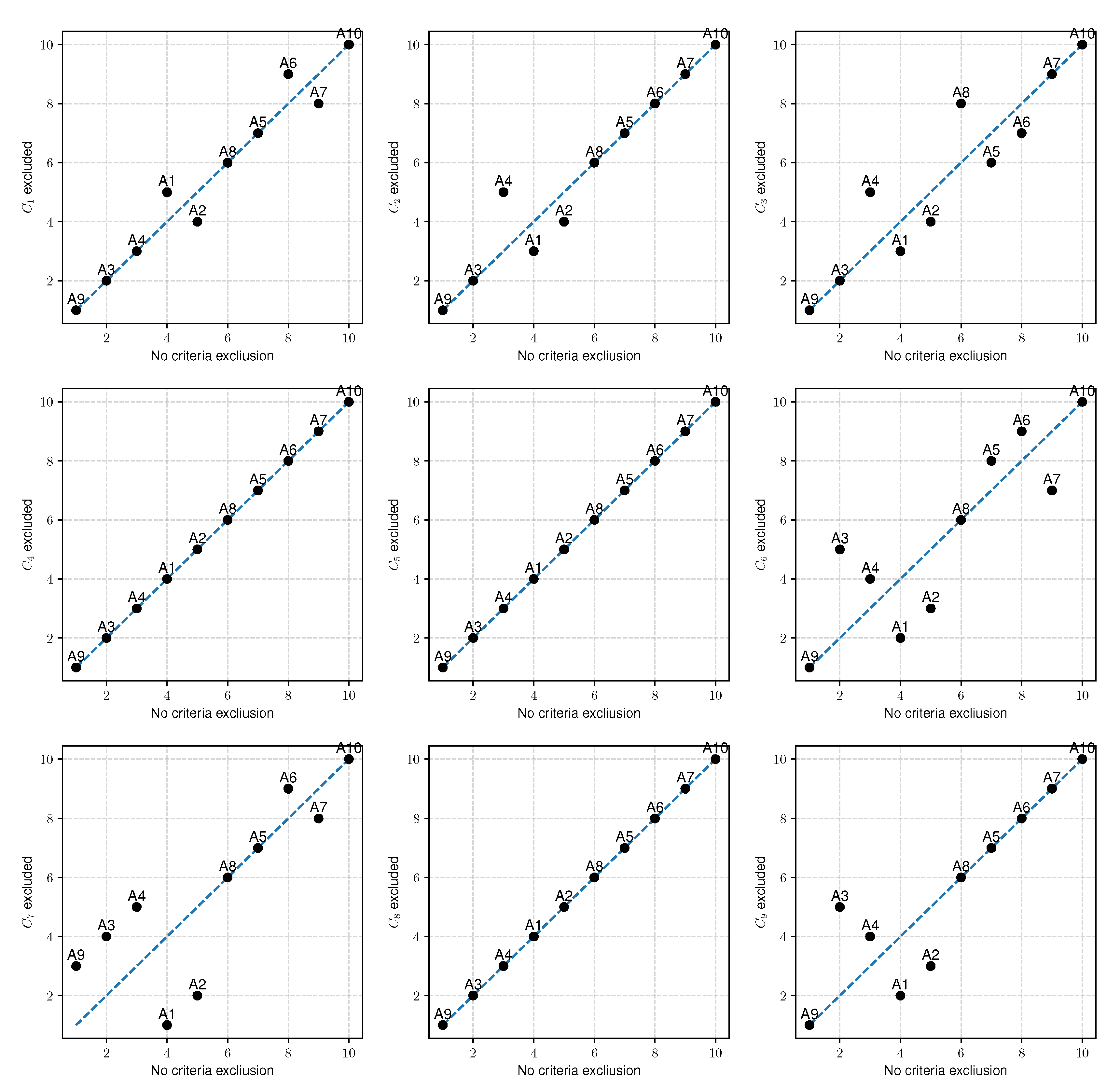
First, we build nine rankings using the monolith COMET approach, one for each criterion excluded, and we calculate $r_w$ and $WS$ correlations between these rankings and ranking obtained with none criterion excluded. We also calculate the euclidean distance between vectors of the preference values, i.e., between the full set of criteria and a set of criteria with exclusions. Results are presented in

Table 7. Ranking similarity coefficients determined for one or more excluded criteria.

Excluding	${\mathit{A}}_1$	${\mathit{A}}_2$	${\mathit{A}}_2$	${\mathit{A}}_2$	${\mathit{A}}_2$	${\mathit{A}}_2$	${\mathit{A}}_2$	${\mathit{A}}_2$	${\mathit{A}}_2$	${\mathit{A}}_2$	${\mathit{r}}_{\mathit{w}}$	$\mathit{WS}$	Distance
none	4	5	2	3	7	8	9	6	1	10	1.0000	1.0000	0.0000
$C_1$	5	4	2	3	7	9	8	6	1	10	0.9802	0.9825	0.2048
$C_2$	3	4	2	5	7	8	9	6	1	10	0.9537	0.9476	0.1083
$C_3$	3	4	2	5	6	7	9	8	1	10	0.9273	0.9395	0.1716
$C_4$	4	5	2	3	7	8	9	6	1	10	1.0000	1.0000	0.1732
$C_5$	4	5	2	3	7	8	9	6	1	10	1.0000	1.0000	0.1600
$C_6$	2	3	5	4	8	9	7	6	1	10	0.8314	0.8527	0.2140
$C_7$	1	2	4	5	7	9	8	6	3	10	0.7300	0.7399	0.2284
$C_8$	4	5	2	3	7	8	9	6	1	10	1.0000	1.0000	0.2093
$C_9$	2	3	5	4	7	8	9	6	1	10	0.8512	0.8551	0.2134
$C_4$, $C_5$	8	9	1	3	5	7	6	4	2	10	0.7333	0.8364	0.3659
$C_4$, $C_8$	8	9	1	3	5	6	7	4	2	10	0.7410	0.8361	0.3958
$C_5$, $C_8$	8	9	2	3	5	6	7	4	1	10	0.7620	0.9229	0.4139
$C_4$, $C_5$, $C_8$	8	9	1	3	5	7	6	4	2	10	0.7333	0.8364	0.6527

.

After the elimination of one criterion, it turned out that excluding criteria $C_4$, $C_5$, or $C_8$ does not influence the ranking. This is surprising because criterion $C_4$ and $C_5$ were indicated as the criteria with the highest relevance for the Pearson correlation coefficient analysis. However, after removing one of them, the ranking remains unchanged, and the value of $r_W$ and $WS$ is 1. The most important criterion, i.e., the one that has the most significant influence on the change of the ranking, turned out to be the criterion $C_7$, which has the smallest value in the Pearson coefficient analysis.

The second most important decision criterion is the $C_6$ criterion, which was also considered to be one of the less important in the Pearson’s coefficient analysis. The criteria $C_6$ and $C_7$ refer to the battery charge time, with the more critical parameter being the time it takes for the cells to recharge to 80% and the less critical parameter being a 100% charge. This is by common sense and the literature on the subject, where the most important challenge for the electric vehicles is the charging time. It depends on it whether the vehicle can move or will stand idle. The third most important criterion is $C_9$, which is the cost of purchase. When we additionally analyze the distances between the vectors of the obtained preferences before and after the reduction of the number of criteria, it turns out that these criteria have the most outstanding value of distance. However, the distance itself seems to be a non-prejudicative predictor as the distance values vary from 0.1600 to 0.2093 for criteria that have not changed the ranking. It is also interesting that the ranking was not influenced by criteria related to engine parameters and battery capacity.

The next step of our analysis is to check the exclusion of all combinations for criteria $C_4$, $C_5$, and $C_8$. Despite the lack of their strong relevance, it turns out that in case of exclusion of two combinations, the model deteriorates significantly and reaches $r_w$ values close to the situation when only the $C_7$ criterion was excluded. In the case of subsequent exclusions, i.e., the three criteria, we have assumed results identical to those of two $C_4$ and $C_5$. However, further analysis of Table 7 shows us that distance between preference vectors is increasing with a number of criteria excluded. Therefore, the excluded triple criteria have equal rankings, but the distance between preference vectors is almost twice time bigger.

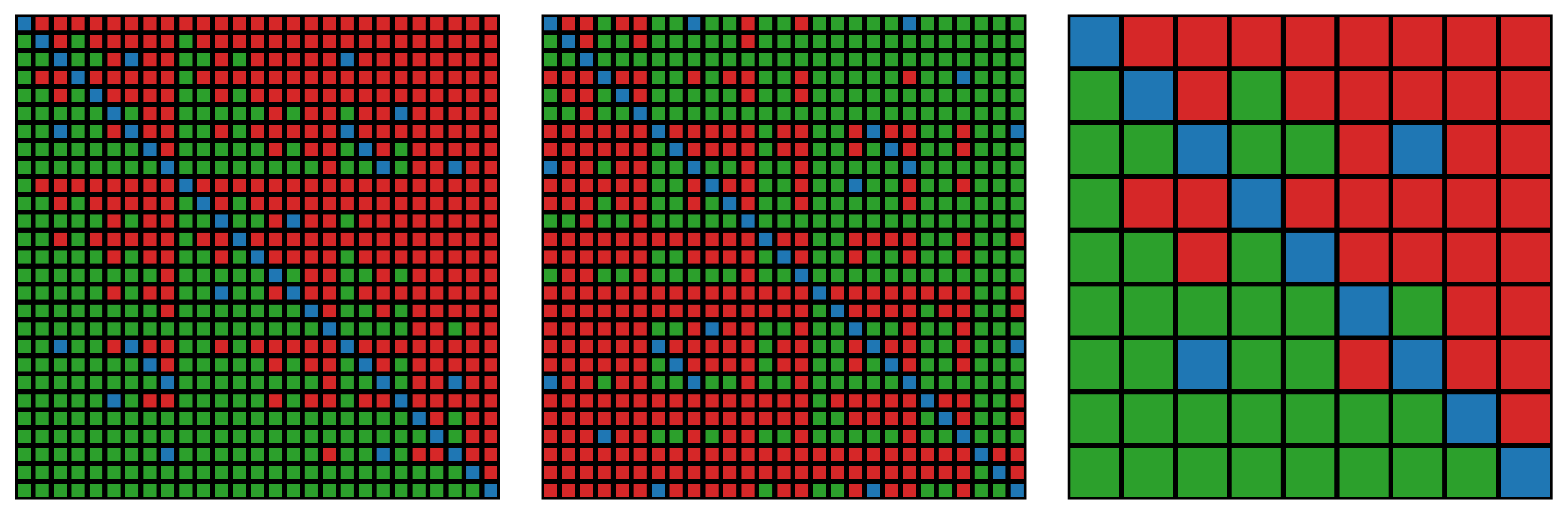
Excluding even three criteria from the monolithic COMET proved to be no more significant than removing the $C_7$ criterion. Figure 8 shows the visualization of changes taking place in the initial ranking when eliminating three criteria from the set of criteria. As it turns out, only the alternatives $A_4$ and $A_{10}$ remained in their places.

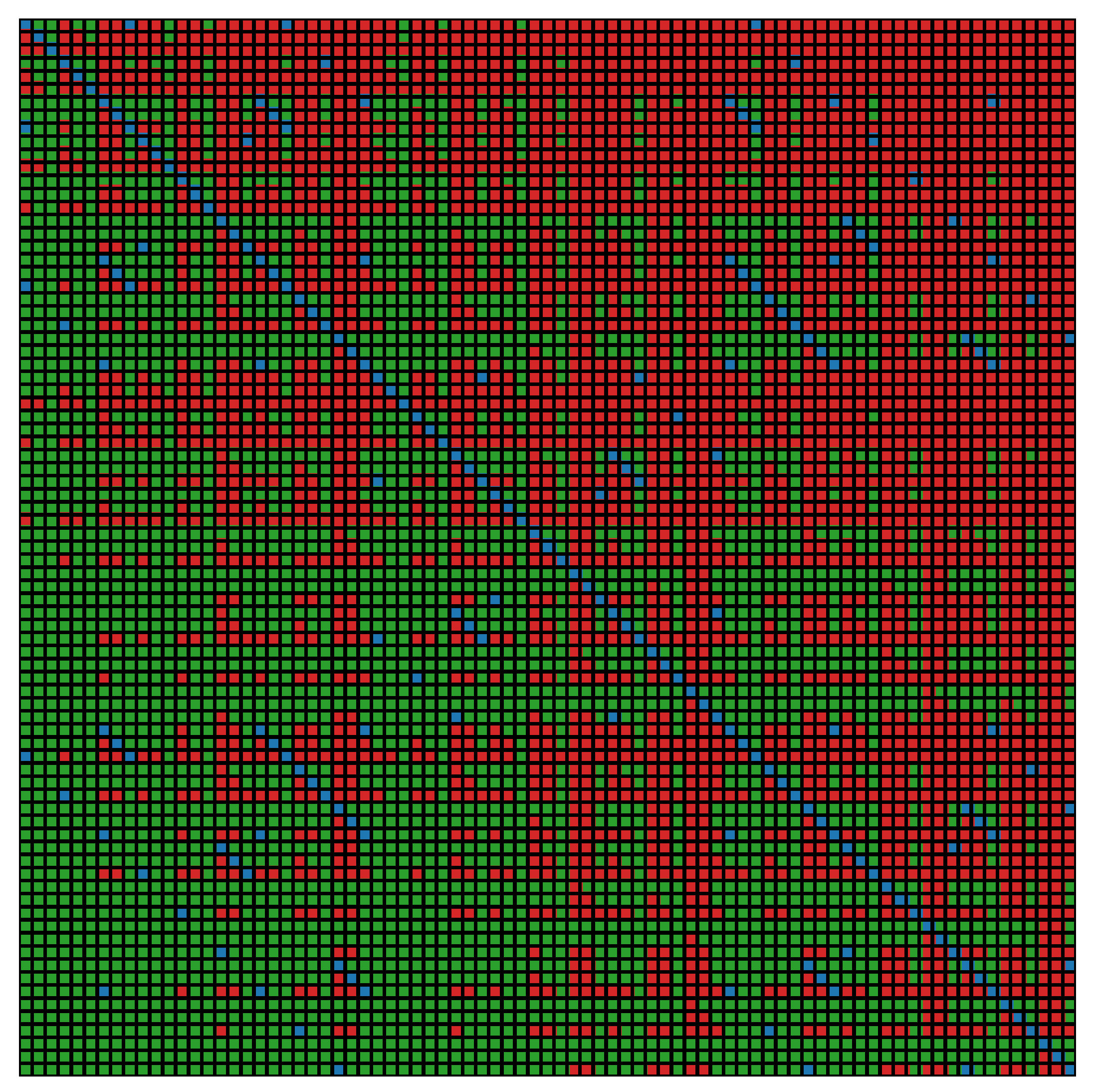
The exclusions of single criteria are presented in Figure 9. The exclusion of criterion $C_7$ causes greater changes at the top of the ranking, while the alternatives $A_5$, $A_8$, and $A_{10}$ remain in place. Figure 8, Figure 9 and Figure 10 show visualization of $r_w$ and $WS$ coefficients, where we can quickly make a comparison between disordered levels.

Figure 10 shows the difference between $WS$ and $r_w$. In all three presented cases, the $r_w$ ratio has a similar value. This is completely different in the case of the $WS$ coefficient, where when excluding the $C_5$ and $C_8$ criteria, we get a relatively high value of 0.9229. Figure 10 shows that is because both rankings have the same top three alternatives in the ranking ($A_{10}$ also does not change position but its importance is marginal and does not exceed $2^{-10}$). In the other two cases, only the alternatives $A_4$ and $A_{10}$ do not change their order with respect to initial raking.

In conclusion, the most significant potential in determining the relevance of criteria has an approach in which we exclude individual criteria from the model and check the impact of this on the similarity of the obtained rankings. Useful indicators for this purpose are both the $r_w$ and $WS$ ratio. The distance between the preference vectors may be helpful, but it is certainly not the most critical factor.

4.3. Incomplete Data

Let us assume that the decision alternative is described with partially incomplete data. There are three examples of alternatives in

Table 8. Sample alternatives with incomplete data and interval preferences.

${\mathit{A}}_{\mathit{i}}$	${\mathit{C}}_1$	${\mathit{C}}_2$	${\mathit{C}}_3$	${\mathit{C}}_4$	${\mathit{C}}_5$	${\mathit{C}}_6$	${\mathit{C}}_7$	${\mathit{C}}_8$	${\mathit{C}}_9$	${\mathit{P}}_{\mathit{monolith}}$	${\mathit{P}}_{\mathit{structured}}$
$A_1$	695	110	170	49	200	7.5	30	22.5	[12.9, 120.0]	[0.3064, 0.4971]	[0.2460, 0.6037]
$A_2$	650	130	170	44	226	8	[10, 120]	22	22.0	[0.3590, 0.5396]	[0.0000, 0.6536]
$A_3$	2500	80	150	90	[80, 610]	7	120	40	81.0	[0.2863, 0.4799]	[0.2881, 0.4500]

, where we do not know the values for criteria $C_5$, $C_7$, and $C_9$ for the alternatives $A_1$, $A_2$, and $A_3$ respectively. Incomplete data makes calculations impossible in this situation because one of the input signals is missing. The only thing we can assume in such a situation is that the value of the attributes is within the scope of our model. Therefore, instead of missing data, we insert intervals that are equal to the extreme characteristic values. Data has already been entered in Table 8. We then calculate preference values using a monolithic and structural approach by calculating all possible combinations. As a result, we get the interval of the lowest and highest possible preference.

In the purpose of ordering the alternatives evaluated by using the interval values, we will use Ishibuchi and Tanaka’s approach [61], where if A = $[a_L;a_R]$ and B = $[b_L;b_R]$ are two interval profits, then the order relation ${\le }_{LR}$ for maximization problems is defined as (28)

$$\begin{array}{cc}A{\le }_{LR}B\hfill & \mathrm{iff}{a}_L\le b_L\mathrm{and}{a}_R\le b_R,\hfill \\ A{<}_{LR}B\hfill & \mathrm{iff}A{\le }_{LR}B\mathrm{and}A\ne B\hfill \end{array}.$$

(28)

We also use the order relation ${\le }_{CW}$ for maximization problems. Let A = $[a_C;a_W]$ and B = $[b_C;b_W]$ be two intervals in center and radius form, then the order relation ${\le }_{CW}$ for maximization problems is defined as (29)

$$\begin{array}{c}A{\le }_{CW}B\mathrm{iff}{a}_C\le b_C\mathrm{and}{a}_w\ge b_w,\hfill \\ A{<}_{CW}B\mathrm{iff}A{\le }_{CW}B\mathrm{and}A\ne B.\hfill \end{array}$$

(29)

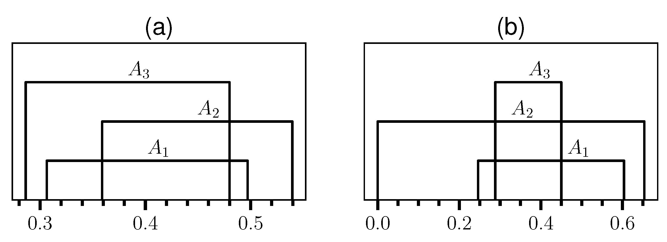
Figure 11 shows the interval results for the monolithic and structured approaches. It seems that we have achieved two different results, i.e., results with different ranking orders. However, applying the approach (28) and (29), respectively, we get two identical rankings, where for monolithic approach we get $A_3{<}_{LR}{A}_1{<}_{LR}{A}_2$ and for structured approach $A_3{<}_{CW}{A}_1{<}_{CW}{A}_2$. Both approaches can be used for calculations with partially incomplete data. However, it should be remembered that these calculations only contain the correct result and do not represent it. This means that only one value in the interval is the real final preference.

5. Conclusions

In this paper, we show two approaches to identify fuzzy models with partially incomplete data. We have compared using two approaches, the monolithic approach, which assumes creating one model, and the structured approach with a decomposed problem on several interrelated models. The main contribution is the comparison of both approaches in terms of accuracy based on the analyzed study case. Additionally, we proposed an effective way to identify the relevance of the criteria. For this purpose, we have applied two ranking similarity coefficients, i.e., $r_w$ and $WS$ coefficients. This approach proved to be more effective than the Pearson correlation analysis between input signals and final alternative preferences.

In the last stage of the research we showed how to use monolithic and structured approaches to decision-making in multicriteria problems with partially incomplete data. Based on an example taken from the literature, we obtained results for the samples of alternatives with incomplete data in the form of interval values. These values are not trivial to interpret, but based on Ishibuchi and Tanaka’s approach we have obtained an identical order of obtained intervals. However, it should be remembered that the received solution is correct, but unfortunately it is a little inaccurate or, to be more precise, such a solution is quite broad. The research confirms the main contribution that both approaches can solve problems with very similar accuracy. The results obtained differed from each other in a statistically insignificant way.

During the research, some improvement areas have been identified. The future work directions should concentrate on

• research of using other number generalizations instead of interval numbers to solve problems with partially incomplete data,
• more extensive research on the accuracy of monolithic and structured approaches using computer simulations, and
• developing a new method to the identification of criteria significance.

References

1. Mulliner, E.; Malys, N.; Maliene, V. Comparative analysis of MCDM methods for the assessment of sustainable housing affordability. Omega 2016, 59, 146–156. [Google Scholar] [CrossRef]
2. Tzeng, G.H.; Chiang, C.H.; Li, C.W. Evaluating intertwined effects in e-learning programs: A novel hybrid MCDM model based on factor analysis and DEMATEL. Expert Syst. Appl. 2007, 32, 1028–1044. [Google Scholar] [CrossRef]
3. Cinelli, M.; Kadziński, M.; Gonzalez, M.; Słowiński, R. How to Support the Application of Multiple Criteria Decision Analysis? Let Us Start with a Comprehensive Taxonomy. Omega 2020, 96, 102261. [Google Scholar] [CrossRef]
4. Wątróbski, J.; Jankowski, J.; Ziemba, P.; Karczmarczyk, A.; Zioło, M. Generalised framework for multicriteria method selection. Omega 2019, 86, 107–124. [Google Scholar] [CrossRef]
5. Faizi, S.; Sałabun, W.; Ullah, S.; Rashid, T.; Więckowski, J. A New Method to Support Decision-Making in an Uncertain Environment Based on Normalized Interval-Valued Triangular Fuzzy Numbers and COMET Technique. Symmetry 2020, 12, 516. [Google Scholar] [CrossRef] [Green Version]
6. Zardari, N.H.; Ahmed, K.; Shirazi, S.M.; Yusop, Z.B. Weighting Methods and Their Effects on Multi-Criteria Decision Making Model Outcomes in Water Resources Management; Springer: Berlin/Heidelberg, Germany, 2015. [Google Scholar]
7. Sengupta, A.; Pal, T.K. On comparing interval numbers. Eur. J. Oper. Res. 2000, 127, 28–43. [Google Scholar] [CrossRef]
8. Dubois, D.; Prade, H. Fuzzy numbers: An overview. In Readings in Fuzzy Sets for Intelligent Systems; Elsevier: Amsterdam, The Netherlands, 1993; pp. 112–148. [Google Scholar]
9. Antoni, L.; Krajči, S.; Krídlo, O. Representation of fuzzy subsets by Galois connections. Fuzzy Sets Syst. 2017, 326, 52–68. [Google Scholar] [CrossRef]
10. Zavadskas, E.K.; Kaklauskas, A.; Turskis, Z.; Tamošaitienė, J. Multi-attribute decision-making model by applying grey numbers. Informatica 2009, 20, 305–320. [Google Scholar] [CrossRef]
11. Utkin, L.V.; Augustin, T. Decision making under incomplete data using the imprecise Dirichlet model. Int. J. Approx. Reason. 2007, 44, 322–338. [Google Scholar] [CrossRef] [Green Version]
12. Wątróbski, J.; Jankowski, J.; Ziemba, P.; Karczmarczyk, A.; Zioło, M. Generalised framework for multicriteria method selection: Rule set database and exemplary decision support system implementation blueprints. Data Brief 2019, 22, 639. [Google Scholar] [CrossRef]
13. Behzadian, M.; Otaghsara, S.K.; Yazdani, M.; Ignatius, J. A state-of the-art survey of TOPSIS applications. Expert Syst. Appl. 2012, 39, 13051–13069. [Google Scholar] [CrossRef]
14. Brans, J.P.; Vincke, P.; Mareschal, B. How to select and how to rank projects: The PROMETHEE method. Eur. J. Oper. Res. 1986, 24, 228–238. [Google Scholar] [CrossRef]
15. Ziemba, P.; Wątróbski, J.; Zioło, M.; Karczmarczyk, A. Using the PROSA method in offshore wind farm location problems. Energies 2017, 10, 1755. [Google Scholar] [CrossRef] [Green Version]
16. Emrouznejad, A.; Marra, M. The state of the art development of AHP (1979–2017): A literature review with a social network analysis. Int. J. Prod. Res. 2017, 55, 6653–6675. [Google Scholar] [CrossRef] [Green Version]
17. Ziemba, P. Inter-criteria dependencies-based decision support in the sustainable wind energy management. Energies 2019, 12, 749. [Google Scholar] [CrossRef] [Green Version]
18. Sipahi, S.; Timor, M. The analytic hierarchy process and analytic network process: An overview of applications. Manag. Decis. 2010. [Google Scholar] [CrossRef]
19. Becker, J.; Becker, A.; Sałabun, W. Construction and use of the ANP decision model taking into account the experts’ competence. Procedia Comput. Sci. 2017, 112, 2269–2279. [Google Scholar] [CrossRef]
20. Opricovic, S.; Tzeng, G.H. Compromise solution by MCDM methods: A comparative analysis of VIKOR and TOPSIS. Eur. J. Oper. Res. 2004, 156, 445–455. [Google Scholar] [CrossRef]
21. Figueira, J.; Mousseau, V.; Roy, B. ELECTRE methods. In Multiple Criteria Decision Analysis: State of the Art Surveys; Springer: Berlin/Heidelberg, Germany, 2005; pp. 133–153. [Google Scholar]
22. Kaklauskas, A.; Zavadskas, E.K.; Raslanas, S.; Ginevicius, R.; Komka, A.; Malinauskas, P. Selection of low-e windows in retrofit of public buildings by applying multiple criteria method COPRAS: A Lithuanian case. Energy Build. 2006, 38, 454–462. [Google Scholar] [CrossRef]
23. Stefano, N.M.; Casarotto Filho, N.; Vergara, L.G.L.; da Rocha, R.U.G. COPRAS (Complex Proportional Assessment): State of the art research and its applications. IEEE Lat. Am. Trans. 2015, 13, 3899–3906. [Google Scholar] [CrossRef]
24. Mendoza, G.A.; Martins, H. Multi-criteria decision analysis in natural resource management: A critical review of methods and new modeling paradigms. For. Ecol. Manag. 2006, 230, 1–22. [Google Scholar] [CrossRef]
25. Palczewski, K.; Sałabun, W. The fuzzy TOPSIS applications in the last decade. Procedia Comput. Sci. 2019, 159, 2294–2303. [Google Scholar] [CrossRef]
26. Ziemba, P.; Becker, A.; Becker, J. A Consensus Measure of Expert Judgment in the Fuzzy TOPSIS Method. Symmetry 2020, 12, 204. [Google Scholar] [CrossRef] [Green Version]
27. Yazdani, M.; Alidoosti, A.; Zavadskas, E.K. Risk analysis of critical infrastructures using fuzzy COPRAS. Econ. Res.-Ekon. Istraž. 2011, 24, 27–40. [Google Scholar] [CrossRef]
28. Fouladgar, M.M.; Yazdani-Chamzini, A.; Lashgari, A.; Zavadskas, E.K.; Turskis, Z. Maintenance strategy selection using AHP and COPRAS under fuzzy environment. Int. J. Strateg. Prop. Manag. 2012, 16, 85–104. [Google Scholar] [CrossRef]
29. Ziemba, P. NEAT F-PROMETHEE—A new fuzzy multiple criteria decision making method based on the adjustment of mapping trapezoidal fuzzy numbers. Expert Syst. Appl. 2018, 110, 363–380. [Google Scholar] [CrossRef]
30. Ziemba, P.; Becker, J. Analysis of the digital divide using fuzzy forecasting. Symmetry 2019, 11, 166. [Google Scholar] [CrossRef] [Green Version]
31. Chang, D.Y. Applications of the extent analysis method on fuzzy AHP. Eur. J. Oper. Res. 1996, 95, 649–655. [Google Scholar] [CrossRef]
32. Ziemba, P. Towards strong sustainability management—A generalized PROSA method. Sustainability 2019, 11, 1555. [Google Scholar] [CrossRef] [Green Version]
33. Naderi, E.; Pourakbari-Kasmaei, M.; Abdi, H. An efficient particle swarm optimization algorithm to solve optimal power flow problem integrated with FACTS devices. Appl. Soft Comput. 2019, 80, 243–262. [Google Scholar] [CrossRef]
34. Kahraman, C.; Onar, S.C.; Oztaysi, B. Fuzzy multicriteria decision-making: A literature review. Int. J. Comput. Intell. Syst. 2015, 8, 637–666. [Google Scholar] [CrossRef] [Green Version]
35. Naderi, E.; Azizivahed, A.; Narimani, H.; Fathi, M.; Narimani, M.R. A comprehensive study of practical economic dispatch problems by a new hybrid evolutionary algorithm. Appl. Soft Comput. 2017, 61, 1186–1206. [Google Scholar] [CrossRef]
36. Sałabun, W. The Characteristic Objects Method: A New Distance-based Approach to Multicriteria Decision-making Problems. J. Multi-Criteria Decis. Anal. 2015, 22, 37–50. [Google Scholar] [CrossRef]
37. Wątróbski, J.; Sałabun, W. Green supplier selection framework based on multicriteria decision-analysis approach. In Smart Innovation, Systems and Technologies, Proceedings of the International Conference on Sustainable Design and Manufacturing, Gold Coast, QLD, Australia, 24–26 June 2016; Springer: Cham, Switzerland, 2016; pp. 361–371. [Google Scholar]
38. Więckowski, J.; Kizielewicz, B.; Kołodziejczyk, J. Application of Hill Climbing Algorithm in Determining the Characteristic Objects Preferences Based on the Reference Set of Alternatives. In Smart Innovation, Systems and Technologies, Proceedings of the International Conference on Intelligent Decision Technologies, Split, Croatia, 17–19 June 2020; Springer: Singapore, 2020; pp. 341–351. [Google Scholar]
39. Więckowski, J.; Kizielewicz, B.; Kołodziejczyk, J. Finding an Approximate Global Optimum of Characteristic Objects Preferences by Using Simulated Annealing. In Smart Innovation, Systems and Technologies, Proceedings of the International Conference on Intelligent Decision Technologies, Split, Croatia, 17–19 June 2020; Springer: Singapore, 2020; pp. 365–375. [Google Scholar]
40. Wątróbski, J.; Sałabun, W.; Karczmarczyk, A.; Wolski, W. Sustainable decision-making using the COMET method: An empirical study of the ammonium nitrate transport management. In Proceedings of the 2017 Federated Conference on Computer Science and Information Systems (FedCSIS), Prague, Czech Republic, 3–6 September 2017; pp. 949–958. [Google Scholar]
41. Wątróbski, J.; Małecki, K.; Kijewska, K.; Iwan, S.; Karczmarczyk, A.; Thompson, R. Multi-Criteria Analysis of Electric Vans for City Logistics. Sustainability 2017, 9, 1453. [Google Scholar] [CrossRef] [Green Version]
42. Zadeh, L. Fuzzy sets. Inf. Control 1965, 8, 338–353. [Google Scholar] [CrossRef] [Green Version]
43. Piegat, A.; Sałabun, W. Comparative analysis of MCDM methods for assessing the severity of chronic liver disease. In Lecture Notes in Computer Science, Proceedings of the International Conference on Artificial Intelligence and Soft Computing, Zakopane, Poland, 14–18 June 2015; Springer: Cham, Switzerland, 2015; pp. 228–238. [Google Scholar]
44. Jankowski, J.; Sałabun, W.; Wątróbski, J. Identification of a multicriteria assessment model of relation between editorial and commercial content in web systems. In Multimedia and Network Information Systems; Springer: Berlin/Heidelberg, Germany, 2017; pp. 295–305. [Google Scholar]
45. Salabun, W.; Napierala, M.; Bykowski, J. The Identification of Multi-Criteria Model of the Signicficance of Drainage Pumping Stations in Poland. Acta Sci. Polonorum. Form. Circumiectus 2015, 14, 147. [Google Scholar] [CrossRef]
46. Faizi, S.; Sałabun, W.; Rashid, T.; Wątróbski, J.; Zafar, S. Group decision-making for hesitant fuzzy sets based on characteristic objects method. Symmetry 2017, 9, 136. [Google Scholar] [CrossRef]
47. Faizi, S.; Rashid, T.; Sałabun, W.; Zafar, S.; Wątróbski, J. Decision making with uncertainty using hesitant fuzzy sets. Int. J. Fuzzy Syst. 2018, 20, 93–103. [Google Scholar] [CrossRef] [Green Version]
48. Sałabun, W.; Karczmarczyk, A. Using the comet method in the sustainable city transport problem: An empirical study of the electric powered cars. Procedia Comput. Sci. 2018, 126, 2248–2260. [Google Scholar] [CrossRef]
49. Sałabun, W.; Karczmarczyk, A.; Wątróbski, J. Decision-Making using the Hesitant Fuzzy Sets COMET Method: An Empirical Study of the Electric City Buses Selection. In Proceedings of the 2018 IEEE Symposium Series on Computational Intelligence (SSCI), Bangalore, India, 18–21 November 2018; pp. 1485–1492. [Google Scholar]
50. Sałabun, W.; Karczmarczyk, A.; Wątróbski, J.; Jankowski, J. Handling Data Uncertainty in Decision Making with COMET. In Proceedings of the 2018 IEEE Symposium Series on Computational Intelligence (SSCI), Bangalore, India, 18–21 November 2018; pp. 1478–1484. [Google Scholar]
51. Sałabun, W.; Urbaniak, K. A new coefficient of rankings similarity in decision-making problems. In Lecture Notes in Computer Science, Proceedings of the International Conference on Computational Science, Amsterdam, The Netherlands, 3–5 June 2020; Springer: Cham, Switzerland, 2020. [Google Scholar]
52. Baure, G.; Dubarry, M. Synthetic vs. real driving cycles: A comparison of electric vehicle battery degradation. Batteries 2019, 5, 42. [Google Scholar] [CrossRef] [Green Version]
53. Timmermans, J.M.; Matheys, J.; Lataire, P.; Van Mierlo, J.; Cappelle, J. A comparative study of 12 electrically assisted bicycles. World Electr. Veh. J. 2009, 3, 93–103. [Google Scholar] [CrossRef]
54. Florez, D.; Carrillo, H.; Gonzalez, R.; Herrera, M.; Hurtado-Velasco, R.; Cano, M.; Roa, S.; Manrique, T. Development of a Bike-Sharing System Based on Pedal-Assisted Electric Bicycles for Bogota City. Electronics 2018, 7, 337. [Google Scholar] [CrossRef] [Green Version]
55. Roemer, F.; Mrosek, M.; Schmalfuss, S.; Lienkamp, M. New approach for an easily detachable electric drive unit for off-the-shelf bicycles. World Electr. Veh. J. 2018, 9, 37. [Google Scholar] [CrossRef] [Green Version]
56. Ling, Z.; Cherry, C.R.; MacArthur, J.H.; Weinert, J.X. Differences of cycling experiences and perceptions between e-bike and bicycle users in the United States. Sustainability 2017, 9, 1662. [Google Scholar] [CrossRef] [Green Version]
57. Jung, H.; Silva, R.; Han, M. Scaling trends of electric vehicle performance: Driving range, fuel economy, peak power output, and temperature effect. World Electr. Veh. J. 2018, 9, 46. [Google Scholar] [CrossRef] [Green Version]
58. Lee, K.; Chae, J.; Kim, J. A courier service with electric bicycles in an Urban Area: The case in Seoul. Sustainability 2019, 11, 1255. [Google Scholar] [CrossRef] [Green Version]
59. Więckowski, J.; Kizielewicz, B.; Kołodziejczyk, J. The Search of the Optimal Preference Values of the Characteristic Objects by Using Particle Swarm Optimization in the Uncertain Environment. In Smart Innovation, Systems and Technologies, Proceedings of the International Conference on Intelligent Decision Technologies, Split, Croatia, 17–19 June 2020; Springer: Singapore, 2020; pp. 353–363. [Google Scholar]
60. Naderi, E.; Narimani, H.; Fathi, M.; Narimani, M.R. A novel fuzzy adaptive configuration of particle swarm optimization to solve large-scale optimal reactive power dispatch. Appl. Soft Comput. 2017, 53, 441–456. [Google Scholar] [CrossRef]
61. Ishibuchi, H.; Tanaka, H. Multiobjective programming in optimization of the interval objective function. Eur. J. Oper. Res. 1990, 48, 219–225. [Google Scholar] [CrossRef]
Figure 1. Visualization of the triangular fuzzy number A (a, m, b).
Symmetry 12 01541 g001
Figure 2. The procedure of the Characteristic Objects METhod (COMET) method.
Symmetry 12 01541 g002
Figure 3. Triangular fuzzy numbers (TFNs) generated for the criteria C 1 C 9 and the preferences P 1 P 3 , where colors mean the following, blue-low, orange-medium, and green-high.
Symmetry 12 01541 g003
Figure 4. Decomposition of a monolithic model to a structured model.
Symmetry 12 01541 g004
Figure 5. Matrix of Expert Judgment (MEJ) matrices for performance (left), battery (center), and engine (right) models, where green 1.0, blue 0.5, and red 0.0 points.
Symmetry 12 01541 g005
Figure 6. MEJ matrices for final model, where green 1.0, blue 0.5, and red 0.0 points.
Symmetry 12 01541 g006
Figure 7. Visualization of Pearson’s correlation coefficients between inputs values ( C 1 C 9 , P 1 P 3 ) and the final preferences ( P s t r , P m o n ).
Symmetry 12 01541 g007
Figure 8. Visualization of changes taking place in the initial ranking when eliminating three criterion from the set of criteria.
Symmetry 12 01541 g008
Figure 9. Visualization of changes taking place in the initial ranking when eliminating one criterion from the set of criteria.
Symmetry 12 01541 g009
Figure 10. Visualization of changes taking place in the initial ranking when eliminating two criterion from the set of criteria.
Symmetry 12 01541 g010
Figure 11. Visualization of preferences for alternatives A 1 A 3 expressed as intervals, where (a) monolithic approach and (b) structured approach.
Symmetry 12 01541 g011