Abstract
The physics of heat and mass transfer from an object in its wake has significant importance in natural phenomena as well as across many engineering applications. Here, we report numerical results on the population density of the spatial distribution of fluid velocity, pressure, scalar concentration, and scalar fluxes of a wake flow past a sphere in the steady wake regime (Reynolds number 25 to 285). Our findings show that the spatial population distributions of the fluid and the transported scalar quantities in the wake follow a Cauchy-Lorentz or Lorentzian trend, indicating a variation in its sample number density inversely proportional to the squared of its magnitude. We observe this universal form of population distribution both in the symmetric wake regime and in the more complex three dimensional wake structure of the steady oblique regime with Reynolds number larger than 225. The population density distribution identifies the increase in dimensionless kinetic energy and scalar fluxes with the increase in Reynolds number, whereas the dimensionless scalar population density shows negligible variation with the Reynolds number. Descriptive statistics in the form of population density distribution of the spatial distribution of the fluid velocity and the transported scalar quantities is important for understanding the transport and local reaction processes in specific regions of the wake, which can be used e.g., for understanding the microphysics of cloud droplets and aerosol interactions, or in the technical flows where droplets interact physically or chemically with the environment.
1. Introduction
The interactions between spherical bodies, such as particles, bubbles, and drops, and the ambient through which they move is a vast area of research, which has attracted attention over centuries in various scientific disciplines [1,2]. The flow past a sphere presents different regimes at different Reynolds number , based on the sphere diameter and the velocity of the incoming flow. The steady axisymmetric structure of a wake at low Reynolds number, up to , was studied experimentally, for example by Teneda (1956) [3] and numerically by Tomboulides and Orszag (2000) [4] among others [5]. The steady axisymmetric regime is followed by a steady oblique wake structure, with up to 280, which was observed experimentally by Magarvey and Bishop (1961) [6] and numerically by Johnson and Patel (1999) [7], for example. An unsteady structure of the wake appears at higher , and was reported by Fornberg (1988) among others [8,9]. The drag coefficient of a sphere, which varies with the roughness of the sphere surface and , was studied in detail, for example, by Eichhorn and Small (1964) and others experimentally [10,11,12,13] and by Tabata and Itakura (1998) [14], Birouk and Al-Sood(2007) [15] numerically. At present, how the drag, lift and pressure coefficients vary both locally as well as globally with respect to the sphere is well known [4,15,16]. The two dimensional structures of the streamlines, vorticity and pressure contours along the orthogonal central planes through the sphere are also well known over various studies, such as, Tomboulides and Orszag (2000) and others [4,7,17].
Many engineering applications and natural processes rely on understanding the interaction between a sphere and the ambient, also involving transport of various scalar species, either passively advected by the ambient flow or interacting actively with the flow through various physical processes, for example, through evaporation and buoyancy. The rate of scalar transport, in particular the convective heat transfer from spherical objects at various , has been investigated both numerically, for example, by Bagchi et al. (2000) [17] and Richter and Nikrityuk (2012) [18] and experimentally by Kramers (1946), among others [19,20,21,22] to determine the heat transfer coefficient. Similar to the drag coefficient, attention was given to the dependence of the local Nusselt number (a ratio of the convective and the diffusive (conductive) heat transfer) on the sphere surface and its global average for different [17,22]. The profiles of the dimensionless temperature contours along the central orthogonal plane for various have also been described in the studies by Bagchi et al. (2000) [17] and Chouippe et al. (2019) [23]. A coupled system involving an interplay between different scalars can also be present, for example, in case of the phase change during droplets evaporation or freezing resulting in heat and mass exchange with the ambient air. Such interactions were also studied both experimentally by Ranz and Marshall Jr. (1952) [24] and Friedlander (1957) [25] and numerically by Dennis et al. (1973) [26] and Chouippe et al. (2019) [23]. All these studies are mainly concerned with the average scalar flux at the surface of the sphere, which determines the mass and temperature change rate of the sphere. However, a detailed description of the wake regarding the spatial evolution of the fluid velocity and scalar populations, including the scalar concentrations and the convective fluxes, both in two and three dimensions for various steady , have not been fully explored.
Descriptive statistics on the spatial structure of the wake is of primary importance if the extent of the wake with certain properties needs to be quantified. Supersaturation in the wake of precipitating cloud water droplets, which have important implications for cloud life cycle as investigated by Bhowmick et al. (2020) [27] and Krayer et al. (2020) [28], requires for example a detailed analysis of the transported scalar population in the wake. To quantify the extent of the supersaturated volume in the wake of a cloud droplet, where aerosols can grow by the deposition of the excess water vapor in the supersaturated wake and can be activated due to sufficiently long exposure to supersaturation in the droplet wake [27]; the details of the scalar population in the wake need to be known with a quantification on the scalar transport and its population distribution. In this paper, we present a comprehensive numerical study on the details of the momentum and scalar transport in the wake of a sphere using a population density distribution for the steady axisymmetric and oblique wake regimes. A brief introduction of the numerical methods and computational details are described in Section 2. Results are presented and discussed in Section 3. Finally, conclusions are given in Section 4.
2. Physical Model, Numerical Method and Boundary Conditions
We consider the flow which develops past a sphere, placed in incompressible viscous fluid with velocity , pressure , and a constant density . Together with the balances of mass and momentum, we also consider the transport of passive scalars, which are any contaminants present in low concentration so that they do not influence the flow. Such dynamics are described in an Eulerian framework by an advection–diffusion (AD) equation. If is the diameter of the sphere, the passive scalar concentration, and are the scalar concentration on the surface of the sphere and in the external flow respectively, the problem can be suitably made dimensionless by using , and as scales, and therefore by defining the dimensionless position, time, velocity, pressure, and scalar concentration as,
Therefore, the dimensionless incompressible Navier-Stokes (NS) equations and the one-way coupled AD equation for the scalar are,
where is the Reynolds number ( is the kinematic viscosity) and is the Schmidt number, the ratio between the kinematic viscosity and the scalar diffusivity . These equations are complemented by uniform flow boundary conditions far from the sphere (, ) and no slip boundary conditions on the surface of the sphere with a constant scalar concentration (, ). From now on the * will be dropped and all variables are in their dimensionless form.
These governing equations are numerically solved with the lattice Boltzmann method (LBM) [29,30]. A code is developed based on the open-source library, Palabos [31]. In LBM, the particle distribution function is governed by
Here i is the index of the discrete velocity , which defines the structure of lattice; and t are the location of a lattice node and the time respectively. The collision operator models the redistribution of the particle populations at each lattice node. In this study, we consider the Bhatnagar-Gross-Krook (BGK) collision operator [32], with which the population relaxes towards its equilibrium state according to the time scale defined below, which determines the relaxation of this equilibration process for the fluid particle distribution function [30]. and are defined as,
Here is the weight, is the speed of sound. The macroscopic quantities, such as the density and velocity are moments of , according to and respectively. For solving the fluid velocity field, the lattice is chosen which is a three dimensional velocity set at each lattice node with one rest-velocity and 18 non-rest velocities. Since the non-linear momentum advection corrections are not very significant in the steady axisymmetric or oblique wake flows, D3Q19 lattice is a good choice for our simulations [33].
The one-way coupling between the fluid momentum and the scalar concentration is solved by another LBM equation similar to Equation (4), but with a distribution function for the scalar. To recover the AD equation, the equilibrium distribution function [34] and the relaxation time scale , which determines the speed of the equilibration process for the scalar distribution function [30], are used as,
The scalar concentration is calculated according to . Since only the zeroth and the first order moments of are used to recover the AD equation from the LBM equation, a lattice is used for solving the scalar field [30].
The sphere is set in the origin of the reference frame, and the dimensionless domain is in size (5 diameters upstream, 20 diameters downstream and 7 diameters in the transversal directions) as shown in Figure 1. The domain is discretized with a uniform Cartesian mesh with a grid size equal to of the sphere diameter. Dirichlet and Neumann boundary conditions are considered for the inlet and outlet boundaries, respectively. For the lateral boundaries in transversal directions, periodic boundary conditions are applied. A second order extrapolation scheme, proposed by Guo et al. (2002) [35], is adopted for the curved boundary of the sphere.
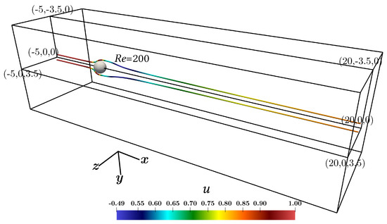
Figure 1.
Sketch of the computational domain used in the simulations. The centre of the sphere is in the origin of the coordinate system. The flow moves from the left to the right in the picture. Two streamlines at Re = 200 are shown as an example.
The numerical setup is validated by comparing the drag coefficient, the length of the recirculating zone, and the angle of separation with the existing research for the fluid velocity field. Mesh independent tests were performed with different mesh spatial resolutions, including , , and . The drag coefficient, the length of the recirculating zone and the angle of separation have shown negligible difference for the grid size of and lower, with maximum variation in the length of the recirculating zone, up to . The domain size independence tests are conducted for various transversal and stream-wise extents of the domain, from to (changing the transversal extent), and from to (changing the stream-wise extent) with grid size . The domains have shown variation only in the length of the recirculating zone, which is up to longer for the wider domain. For example, in Figure 2a, the drag coefficient obtained from our simulation is compared with empirical equations (Equations (5) and (6)) of Clift et al. (1978) [1] and with the numerical results of Johnson and Patel (1999) [7]. The drag coefficient deviates from the empirical equations maximum at , with relative error , which is further reduced with higher , e.g., less than at . Figure 2b presents the results of the normalized wake length along with the numerical results of Johnson and Patel (1999) [7], Tomboulides and Orszag (2000) [4], and experimental data of Taneda (1956) [3], which reported transition to unsteady wake for . The scalar field is validated by comparing the normalized scalar profiles with other numerical simulations, which for example shows a maximum of 2 lattice node difference from the temperature profiles of Chouippe et al. (2019) [23] at a similar scalar diffusivity of (not shown here).
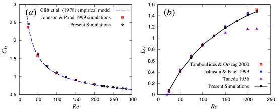
Figure 2.
(a) Drag coefficient and (b) wake length normalized with sphere diameter for various steady axisymmetric and oblique with existing research [1,3,4,7].
3. Results on Spatial Structure of Steady Wake
Our work focuses on the wake behind a wet sphere in the steady axisymmetric regime () and the steady oblique regime (). The difference in the overall features of these regimes can be appreciated from Figure 3, which visualizes the stream-wise velocity u in color together with the contours of two advected scalar fields in black and in white of different scalar diffusivities in two perpendicular planes () and () passing through the center of sphere in parallel to the incoming flow. The Schmidt numbers for the scalars are 0.71 and 0.61, respectively, which correspond to the diffusivities of temperature and water vapor in air. The increase in features the thinning of the boundary layer, as well as a shrinking in the lateral extent of the wake and a stretching in the stream-wise direction as in Figure 3 up to . In the oblique regime, a tilt from the centerline () along the () plane is observed, which is symmetric along () plane, see also [7,23]. This tilt in the oblique regime increases with until the wake becomes unstable and starts shedding vortices at . The apparent decrease in the stream-wise length of the wake in the top panel of Figure 3 from to 275 is attributed to the tilting of the wake. The transport of any scalar is described by the same Equation (3). The only difference lays in their Schmidt numbers, which govern their relative diffusivities. The different diffusivities govern the profiles of the scalars at the intermediate values of the dimensionless concentration, which shows difference in the external part away from the sphere boundary and in the far wake (for to ), as shown in Figure 3. Due to the Schmidt numbers, the gradient of is less steep than the gradient of . This feature, however, becomes less distinctive at higher concentrations of and near the sphere surface.
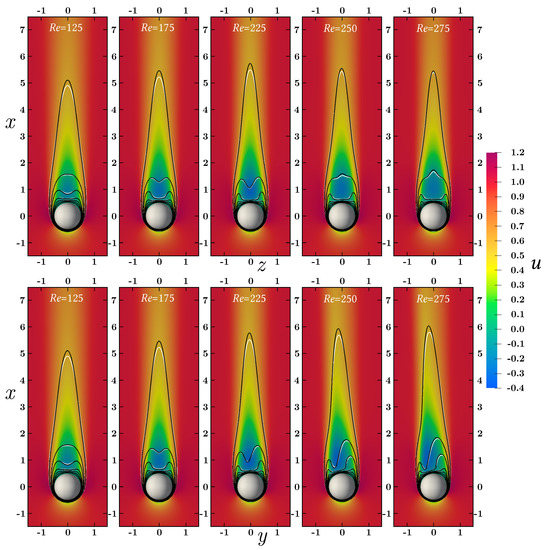
Figure 3.
Spatial distribution of the dimensionless stream-wise component of fluid velocity u in color and the contour lines of a scalar in black () and another scalar in white () for various steady axisymmetric and oblique . The visualization is across two central orthogonal planes () and () passing through the center of the sphere with an extent of [−1.5,1.5] along the horizontal axes and [−1.5,7.5] along the vertical x axis. Contour lines for and are plotted at magnitudes of and , ascending from the ambient towards the sphere.
To provide a detailed description of the flow field, we use a population density approach. For any variable, such as the longitudinal velocity component u, its population density distribution at a magnitude is defined as , where is the volume of the region in which u is lower that . The distribution of u is shown in Figure 4 for three different Reynolds numbers (75, 175 and 275). Figure 4a,b present the contour lines of in solid lines and of pressure in dashed thin lines across the () and () orthogonal planes respectively. The domain can be divided into two main parts: an upstream zone where the flow approaches the sphere and a downstream zone dominated by the presence of the wake. The dotted horizontal black line in panels a and b of Figure 4, located at , intersects the sphere where the dimensionless pressure p changes sign and distinguishes the two zones. The velocity component u in the upstream zone () does not show significant changes with , but the above mentioned lateral thinning is visible in the downstream zone, which has mostly negative p. Tilting is also observed in Figure 4b for .
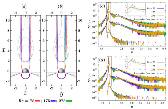
Figure 4.
Distribution of the dimensionless stream-wise velocity component u for various . contours are drawn in solid lines along with pressure contours in dashed thin lines along the orthogonal (a) () and (b) () planes. A horizontal dotted line at is drawn to divide the upstream spatial structure of u from the downstream one. Normalized population density function (A is the area of the orthogonal plane) for the u sample population across the orthogonal () and () planes are plotted respectively in (c,d). for the upstream, downstream and the entire planes are respectively plotted as the bottom, middle and the top sets of curves. A scale difference is created by amplifying the of the downstream and the entire domain 30 and 900 times respectively. Sample extent in (a,b) is along the horizontal and along the vertical axes, whereas, in (c,d) it is along the horizontal and along the vertical axes.
Figure 4c,d presents the population density distribution of the longitudinal velocity component u in these two zones, computed along the entire orthogonal () and () planes of the computational domain, respectively. The distribution was determined by dividing the range of u in 1000 bins, a resolution which allows for a smooth sample distribution while preserving its trend. In the upstream zone (bottom sets of curves in Figure 4c,d, shows a sharp decrease in population density as u decreases from the external ambient value of 1 towards the no-slip zero boundary condition at the sphere surface following a Lorentzian function, given in Equation (7). Some sample population with is also observed which resembles the region of highest velocity magnitudes near the contour line. To create a visible scale separation, the of the downstream zone is shifted for the middle set of curves in Figure 4c,d. Negative values of velocity identify the recirculation zone behind the sphere. A large extent of the simulated wake can be well fitted by a Lorentzian distribution. The crescent-like trend right after the ambient is a result of the finite size of the simulation domain. Similar to the of the upstream zone, some sample population with is also observed in this downstream distribution, which are also coming from the region. of the entire plane is shifted for the top sets of curves in Figure 4c,d with an amplification of its original magnitudes. As plotted in the insets, the two highest peaks at of the entire plane are the individual contributions from both the upstream and the downstream populations.
The Lorentzian or Cauchy-Lorentz distribution is a single peak bell-shaped curve, defined as
where is the population density of samples of variable u, A is its integral over all possible values of u, is the position of its maximum where y takes the value , with b being the width between its half maximums. Parameter is just an offset value, which allows for a non zero asymptotic limit of the Cauchy-Lorentz distribution. In the distribution of u, Figure 4c,d, a Lorentzian trend is observed in the intermediate range, which corresponds to the boundary layer and to the region external to the wake. An increase in is observed with increasing Reynolds numbers, indicating an increase in the dimensionless kinetic energy in this region. The out of plane tilting induced by the oblique wake at produces small spikes on top of an overall Lorentzian trend of the sample population along the () plane, as seen in Figure 4d. However, the oblique wake regime retains a symmetric structure along the () plane in our simulations in Figure 4c but the out of plane tilting impacts the sample population. Therefore, in Figure 4c for only indicates a lower yet a smooth Lorentzian trend.
The existence of such a trend in the distribution of a variable indicates the existence of a matching region where the variable shows an algebraic variation from the values in the wake to the values in the external ambient. If the flow is axisymmetric and the flow structures are elongated in the stream-wise direction, this variation is in the radial direction proportional to (inverse of the square of the lateral distance from the axis). This algebraic matching region is not only present in the longitudinal velocity field, but also in the associated pressure field and in the passively transported scalars.
Figure 5 presents the spatial distribution of the pressure p and the transversal component of velocity v along the orthogonal () plane for various . In the axisymmetric regime, in Figure 5a, the modulus of v is symmetric across the plane but not the v. Similarly the modulus of w is also symmetric across the plane in the axisymmetric regime, but not w. Complexity arises in the oblique regime, as neither p nor the modulus of v remains symmetric in Figure 5b. This is also seen in the population density distribution of v in Figure 5d, where the positive magnitudes of v show dominance similar to Figure 5b. The transversal components of velocity v and w, however, do not show a Lorentzian distribution in its number density. It can be seen in Figure 5a,b that the population of v for the similar magnitudes is present in three different locations which resulted in non-Lorentzian evolution in the number density of the v and w (shown in Figure 5c for v). In contrast to v, the positive and negative magnitudes of p are rather concentrated near the sphere respectively in the upstream and the downstream zones as in Figure 5a,b. Similar to Figure 4c,d, the of the upstream zone ( population) does not show significant variability with and exhibits a Lorentzian distribution. The of the downstream zone however shows local peaks at around , which marks the discontinuity in the sample population in Figure 5a,b.
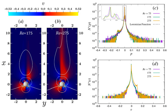
Figure 5.
Distribution of the pressure p and velocity component v for various . The spatial distribution of v in color along with the contour lines of p at magnitudes respectively in red, orange, white, cyan, and blue solid lines along the orthogonal () plane for the axisymmetric in (a) and for the oblique in (b). Normalized population density of pressure across the entire orthogonal () central plane is plotted in (c), whereas is plotted in (d). The sample extent is similar to Figure 4.
A three dimensional spatial structure of the velocity components v and w for the oblique and the axisymmetric cases are shown in Figure 6, where the complexity in the oblique wake flow structure can be appreciated. The previously mentioned symmetry in the modulus of v and w is confirmed in Figure 6d for the steady axisymmetric flow with ; and the three different zones with similar magnitudes of v and w, both positive and negative, can also be seen. The transition to a complex flow structure for the steady oblique case is seen in Figure 6a–c, where the spatial distributions of v and w show differences. Despite the structural differences, both the v and w populations are symmetric along the () planes but non-symmetric along the () planes, which is typical of the steady oblique regime.
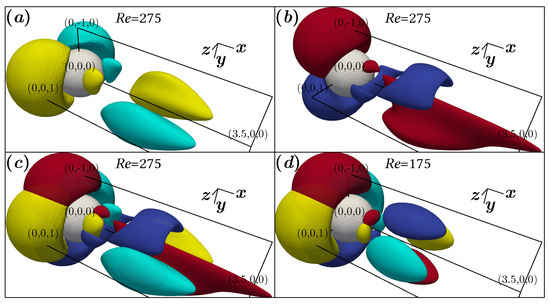
Figure 6.
Three dimensional spatial structure of velocity components, v and w. The surface contours of and are plotted respectively in cyan and yellow in (a), and and contours are plotted respectively in blue and red in (b). (c,d) present both the v and w contours for the oblique and axisymmetric flow fields respectively.
Figure 7 presents the population density distribution of the scalar fields and across two central orthogonal planes () and () (similar to the previous Figures). Since the boundary conditions for the dimensionless scalars have a zero value in the ambient and a unit value on the sphere surface, their population density distribution shows the highest population around zero in Figure 7, followed by a domain induced crescent zone, and then a Lorentzian distribution in the intermediate values gradually approaching the surface unit value. The Lorentzian trend is again visible in the scalar population density, due to the similitude of the advection-diffusion equation for the scalars to the dynamics of momentum in regions with small pressure gradients. In the upstream region, the behaviour of velocity and scalars is very different due to the strong pressure gradient, while in the downstream region the difference is much milder. A closer look at the density distributions in the insets show that the steady axisymmetric cases do not show a well distinguishable difference in the number density at different scalar magnitudes with the increase in , but only the threshold magnitude for the start of the Lorentzian trend increases. The shift in the threshold of Lorentzian trend is attributed due to the finite and a similar size of the simulation domain for all the cases and due to the shrink in the lateral extent of the wake but a stretch in the stream-wise direction with increasing . The decrease in the sample population for the oblique cases in the left panel of Figure 7 for the orthogonal () plane is however due to the out of plane tilt of the wake which reduces the sample population. Whereas in the right panel for the orthogonal () plane, we see a step-wise perturbation on top of an overall Lorentzian trend in the oblique wake regime as a result of its tilt in this plane.
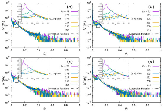
Figure 7.
Spatial evolution of the normalized population density of scalar along the () plane is presented in (a) and along the () plane in (b). Evolution along the () plane is plotted in (c) and along the () plane in (d). These orthogonal planes pass through the center of the sphere and extends to the entire simulated domain of [-3.5:3.5] in the horizontal , and [-5:20] in the stream-wise x directions.
Figure 8 presents the spatial distribution of the convective scalar flux in the stream-wise direction x, which is a product between and u. Spatial distribution of along the orthogonal () plane in Figure 8a,b is someway different from the other flow quantities, since it shows highest positive in the boundary layers and a negative in the recirculating zone due to negative u. The non-symmetric spatial structure of the oblique () scalar flux is visible in Figure 8b. The population density distribution along the orthogonal () and () planes shows a different structure as expected. A Lorentzian trend is observed for a few limited sample populations, for example, for the samples between the white and pink contour lines in Figure 8a,b respectively for and 275. These two contour lines correspond to the magnitudes from Figure 8d marking the beginning and the end of the Lorentzian trend for each individual . Overall an increase in the sample population of is observed with increasing within the zone with Lorentzian distribution.
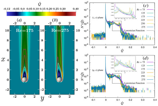
Figure 8.
Spatial distribution of convective scalar flux for various . Spatial distribution of in color along the orthogonal () plane for the axisymmetric in (a) and for the oblique in (b). The white contour lines represent in (a) and in (b), while the pink contour lines are at in (a) and in (b) respectively. Normalized population density of convective scalar flux across the entire orthogonal () and () central planes are plotted respectively in (c,d). The sample extent is similar to Figure 4.
4. Discussions and Concluding Remarks
We present a detailed numerical analysis on the spatial structure of the wake flow using population density distribution for various Reynolds number in the steady wake regime. The incompressible Navier-Stokes equation is solved for the flow velocity and the one-way coupled advection-diffusion equations are solved for the scalars using the Lattice Boltzmann Method (LBM). The spatial evolution of various flow quantities, such as, longitudinal velocity component u, pressure p, passive scalar , convective scalar flux in the wake of the steady axisymmetric regime () and the oblique regime () using a population distribution function N, shows a Lorentzian distribution which is proportional to the inverse of the square of the flow quantity (for example, ). This Lorentzian trend exhibits an algebraic decay in the number density of populations with different magnitudes of fluid quantities from the external ambient to the boundary layer in the wake and dominates the spatial distribution of the flow quantities outside the recirculating region. The transversal components of fluid velocity, v and w, whereas show different spatial distributions not attributable to a Lorentzian one. Transition to the oblique wake regime at in our simulations shows a complex three dimensional spatial evolution of the flow quantities, which also show a Lorentzian trend. The population density distribution for the longitudinal velocity component u, shows an increase in its number density with increasing . Whereas the number density of the scalar populations remains the same for various steady axisymmetric . This feature however changes in case of the convective scalar flux, where an increase in its number density is observed again with an increase in .
Descriptive statistics in the form of population density distributions of the fluid velocity and the transported scalar quantities in the wake of a sphere is important for understanding the transport and local reaction processes in specific regions of the wake. This can be used e.g., for understanding the microphysics of cloud droplets and aerosol interactions, but should also find applications in engineering flows e.g., in which droplets interact with their environment. In cloud physics, the quantification of scalar transport in the wake of spherical hydrometeors was used by Bhowmick et al. (2020) [27] to understand the spatial distribution of supersaturation in the wake of precipitating cloud hydrometeors. In the future, we plan to extend this methodology to study the influence of wake-induced supersaturation on aerosol activation within clouds, by introducing microphysical models for different steady-state and transient wake regimes and studying their effects on the life cycle of clouds. Moreover, as mentioned earlier, our findings will also have application in process engineering, where droplets interact with the environment physically or chemically.
Author Contributions
Conceptualization, T.B., Y.W., M.I., G.B. and E.B.; methodology, T.B., Y.W., M.I., G.B. and E.B.; software, T.B. and Y.W.; simulation, T.B.; investigation, T.B., Y.W., M.I., G.B. and E.B.; visualization, T.B., Y.W., M.I. and G.B.; writing-original draft, T.B., Y.W., M.I., G.B. and E.B.; writing—review and editing, T.B., Y.W., M.I., G.B. and E.B.; supervision, Y.W., M.I., G.B. and E.B.; project administration, Y.W., G.B. and E.B.; funding acquisition, E.B. All authors have read and agreed to the published version of the manuscript.
Funding
This research was funded by the Marie—Skłodowska Curie Actions (MSCA) under the European Union’s Horizon 2020 research and innovation programme (grant agreement no. 675675), and an extension to programme COMPLETE by the Department of Applied Science and Technology, Politecnico di Torino.
Acknowledgments
Scientific activities are carried out in Max Planck Institute for Dynamics and Self-Organization (MPI-DS) and computational resources from HPC@MPIDS are gratefully acknowledged. Scientific comments and suggestions from the reviewers are also gratefully acknowledged. First author wishes to acknowledge Giuliana Donini, Guido Saracco, Mario Trigiante and Paolo Fino for support.
Conflicts of Interest
The authors declare no conflict of interest. The funding sponsors had no role in the design of the study; in the collection, analyses, or interpretation of data; in the writing of the manuscript, or in the decision to publish the results.
References
- Clift, R.; Grace, J.; Weber, M. Bubbles, Drops, and Particles; Academic Press: New York, NY, USA, 1978. [Google Scholar]
- Michaelides, E.E. Particles, Bubbles and Drops; World Scientific: Singapore, 2006. [Google Scholar] [CrossRef]
- Taneda, S. Experimental Investigation of the Wake behind a Sphere at Low Reynolds Numbers. J. Phys. Soc. Jpn. 1956, 11, 1104–1108. [Google Scholar] [CrossRef]
- Tomboulides, A.G.; Orszag, S.A. Numerical investigation of transitional and weak turbulent flow past a sphere. J. Fluid Mech. 2000, 416, 45–73. [Google Scholar] [CrossRef]
- Natarajan, R.; Acrivos, A. The instability of the steady flow past spheres and disks. J. Fluid Mech. 1993, 254, 323–344. [Google Scholar] [CrossRef]
- Magarvey, R.H.; Bishop, R.L. Transition Ranges for Three-Dimensional Wakes. Can. J. Phys. 1961, 39, 1418–1422. [Google Scholar] [CrossRef]
- Johnson, T.A.; Patel, V.C. Flow past a sphere up to a Reynolds number of 300. J. Fluid Mech. 1999, 378, 19–70. [Google Scholar] [CrossRef]
- Fornberg, B. Steady viscous flow past a sphere at high Reynolds numbers. J. Fluid Mech. 1988, 190, 471–489. [Google Scholar] [CrossRef]
- Ormières, D.; Provansal, M. Transition to Turbulence in the Wake of a Sphere. Phys. Rev. Lett. 1999, 83, 80–83. [Google Scholar] [CrossRef]
- Bodenschatz, E.; Eckert, M. Prandtl and the göttingen school. In A Voyage Through Turbulence; Davidson, P.A., Kaneda, Y., Moffatt, K., Sreenivasan, K.R., Eds.; Cambridge University Press: Cambridge, UK, 2011; pp. 40–100. [Google Scholar] [CrossRef]
- Roos, F.W.; Willmarth, W.W. Some experimental results on sphere and disk drag. AIAA J. 1971, 9, 285–291. [Google Scholar] [CrossRef]
- Eichhorn, R.; Small, S. Experiments on the lift and drag of spheres suspended in a Poiseuille flow. J. Fluid Mech. 1964, 20, 513–527. [Google Scholar] [CrossRef]
- Unnikrishnan, A.; Chhabra, R.P. An experimental study of motion of cylinders in newtonian fluids: Wall effects and drag coefficient. Can. J. Chem. Eng. 1991, 69, 729–735. [Google Scholar] [CrossRef]
- Tabata, M.; Itakura, K. A Precise Computation of Drag Coefficients of a Sphere. Int. J. Comput. Fluid Dyn. 1998, 9, 303–311. [Google Scholar] [CrossRef]
- Birouk, M.; Al-Sood, M.M.A. Numerical Study of Sphere Drag Coefficient in Turbulent Flow at Low Reynolds Number. Numer. Heat Transf. Part A Appl. 2007, 51, 39–57. [Google Scholar] [CrossRef]
- Wu, J.; Shu, C. Simulation of three-dimensional flows over moving objects by an improved immersed boundary–lattice Boltzmann method. Int. J. Numer. Methods Fluids 2012, 68, 977–1004. [Google Scholar] [CrossRef]
- Bagchi, P.; Ha, M.Y.; Balachandar, S. Direct Numerical Simulation of Flow and Heat Transfer From a Sphere in a Uniform Cross-Flow. J. Fluids Eng. 2000, 123, 347–358. [Google Scholar] [CrossRef]
- Richter, A.; Nikrityuk, P.A. Drag forces and heat transfer coefficients for spherical, cuboidal and ellipsoidal particles in cross flow at sub-critical Reynolds numbers. Int. J. Heat Mass Transf. 2012, 55, 1343–1354. [Google Scholar] [CrossRef]
- Kramers, H. Heat transfer from spheres to flowing media. Physica 1946, 12, 61–80. [Google Scholar] [CrossRef]
- Gibson, C.H.; Chen, C.C.; Lin, S.C. Measurements of turbulent velocity and temperature fluctuations in the wake of a sphere. AIAA J. 1968, 6, 642–649. [Google Scholar] [CrossRef]
- Yuge, T. Experiments on Heat Transfer From Spheres Including Combined Natural and Forced Convection. J. Heat Transf. 1960, 82, 214–220. [Google Scholar] [CrossRef]
- Will, J.; Kruyt, N.; Venner, C. An experimental study of forced convective heat transfer from smooth, solid spheres. Int. J. Heat Mass Transf. 2017, 109, 1059–1067. [Google Scholar] [CrossRef]
- Chouippe, A.; Krayer, M.; Uhlmann, M.; Dušek, J.; Kiselev, A.; Leisner, T. Heat and water vapor transfer in the wake of a falling ice sphere and its implication for secondary ice formation in clouds. New J. Phys. 2019, 21, 043043. [Google Scholar] [CrossRef]
- Ranz, W.E.; Marshall, W.R. Evaporation from drops: Part I and II. Chem. Eng. Program 1952, 48, 141–146. [Google Scholar]
- Friedlander, S.K. Mass and heat transfer to single spheres and cylinders at low Reynolds numbers. AIChE J. 1957, 3, 43–48. [Google Scholar] [CrossRef]
- Dennis, S.C.R.; Walker, J.D.A.; Hudson, J.D. Heat transfer from a sphere at low Reynolds numbers. J. Fluid Mech. 1973, 60, 273–283. [Google Scholar] [CrossRef]
- Bhowmick, T.; Wang, Y.; Iovieno, M.; Bagheri, G.; Bodenschatz, E. Supersaturation in the Wake of a Precipitating Hydrometeor and its Impact on Aerosol Activation. Earth Space Sci. Open Arch. 2020, 1–13. [Google Scholar] [CrossRef]
- Krayer, M.; Chouippe, A.; Uhlmann, M.; Dušek, J.; Leisner, T. On the ice-nucleating potential of warm hydrometeors in mixed-phase clouds. Atmos. Chem. Phys. Discuss. 2020, 1–21. [Google Scholar] [CrossRef]
- Succi, S. Lattice Boltzmann Equation for Fluid Dynamics and Beyond; Clarendon Press: Oxford, UK, 2001. [Google Scholar]
- Krüger, T.; Kusumaatmaja, H.; Kuzmin, A.; Shardt, O.; Silva, G.; Viggen, E.M. Lattice Boltzmann Method: Fundamentals and Engineering Applications with Computer Codes; Springer: Cham, Switzerland, 2017. [Google Scholar] [CrossRef]
- Latt, J.; Malaspinas, O.; Kontaxakis, D.; Parmigiani, A.; Lagrava, D.; Brogi, F.; Belgacem, M.B.; Thorimbert, Y.; Leclaire, S.; Li, S.; et al. Palabos: Parallel Lattice Boltzmann Solver. Comput. Math. Appl. 2020, 1–17. [Google Scholar] [CrossRef]
- Qian, Y.; D’Humières, D.; Lallemand, P. Lattice BGK models for Navier-Stokes equation. Europhys. Lett. 1992, 17, 479–484. [Google Scholar] [CrossRef]
- Silva, G.; Semiao, V. First- and second-order forcing expansions in a lattice Boltzmann method reproducing isothermal hydrodynamics in artificial compressibility form. J. Fluid Mech. 2012, 698, 282–303. [Google Scholar] [CrossRef]
- Guo, Z.; Shi, B.; Zheng, C. A coupled lattice BGK model for the Boussinesq equations. Int. J. Numer. Methods Fluids 2002, 39, 325–342. [Google Scholar] [CrossRef]
- Guo, Z.; Zheng, C.; Shi, B. An extrapolation method for boundary conditions in lattice Boltzmann method. Phys. Fluids 2002, 14, 2007–2010. [Google Scholar] [CrossRef]
© 2020 by the authors. Licensee MDPI, Basel, Switzerland. This article is an open access article distributed under the terms and conditions of the Creative Commons Attribution (CC BY) license (http://creativecommons.org/licenses/by/4.0/).