Conformal Invariance of Characteristic Lines in a Class of Hydrodynamic Models

Abstract

This paper addresses the problem of the existence of conformal invariance in a class of hydrodynamic models. For this we analyse an underlying transport equation for the one-point probability density function, subject to zero-scalar constraint. We account for the presence of non-zero viscosity and large-scale friction. It is shown analytically, that zero-scalar characteristics of this equation are invariant under conformal transformations in the presence of large-scale friction. However, the non-zero molecular diffusivity breaks the conformal group (CG). This connects our study with previous observations where CG invariance of zero-vorticity isolines of the 2D Navier–Stokes equation was analysed numerically and confirmed only for large scales in the inverse energy cascade. In this paper, an example of CG is analysed and possible interpretations of the analytical results are discussed.

1. Introduction

More than two decades ago A. M. Polyakov (see Ref. [1]) suggested a programme to expand the symmetries admitted by hydrodynamic models to the conformal invariance of equations describing two-dimensional hydrodynamic turbulence. In this case, the conformal group is infinite-dimensional, which enables us to obtain the substantial information on turbulence statistics as it has been done in the Conformal Field Theory [2].

In 3D turbulent flows, the energy is transported in a cascade process from the largest down to the smallest eddies where it is dissipated by viscous effects. In the case of thin layers of fluid, where, possibly, stable stratification and/or rotation additionally suppress vertical motions, these flows share certain common properties with 2D turbulence. In particular, an inverse energy cascade, from smaller to larger eddies is possible and could enhance the formation of stable large-size structures. Two examples are flows of thin soap films [3], where the horizontal-to-vertical aspect ratio is large (${10}^4$) and atmospheric or oceanic flows [4], where the dominant role of Coriolis force, balanced by pressure gradients leads to the development of geostrophic turbulence.

Studies by Bernard et al. [5] on 2D turbulence confirmed that the statistics of zero-vorticity boundaries of large vorticity clusters are conformally invariant. This was done by analysis of the fractal structure of these isoline curves, see for details [5,6] and also review [7]. It was shown numerically that zero-vorticity isolines belong to the class of conformally invariant curves that can be mapped into a one-dimensional Brownian walk called Schramm–Löwner evolution ($SL{E}_{\kappa }$) curves [8] with diffusion coefficient $\kappa =6$. However, this property was not observed at small scales. It was hence argued, the CG is present only in the inverse cascade regime, observed for scales larger than the forcing scale, but it is broken in the direct enstrophy cascade at smaller scales. A theoretical explanation of these observations based on underlying equations is still missing.

A step towards analytical confirmation of CG in 2D turbulence was obtained in [9] using a group-theoretical method developed in [10]. Therein we performed a Lie group analysis of the first equation from the infinite Lundgren–Monin–Novikov (LMN) hierarchy [11,12,13] for the probability density functions (pdfs) of vorticity, with the assumptions of zero viscosity, zero friction and no forcing. These studies can be placed in the broader context of the search for new symmetries in the statistical approach [14,15,16]. In Ref. [9], we showed that the $CG$ is generally broken for the first LMN equation, apart from points on the associated characteristic with zero-vorticity. Notice that the characteristics of the LMN chain exhibit a direct analogy to the Lagrangian description of turbulence. Specifically, the characteristic equations describe the dynamics of the statistics of a class of fluid particles. This Lagrangian point of view was further taken in Ref. [17], where the $CG$ invariance of the Lagrangian path along the zero-vorticity characteristics was established.

In the above-mentioned publications, we also proved the $CG$ invariance of the normalisation and reduction properties, the separation and coincidence properties of the pdfs. We showed that the infinitesimal operator admitted by the characteristic equations forms an infinite-dimensional Lie algebra and a Lie pseudo-group G, which acts as the conformal group on a domain $D_1\subset R^2$.

To link these findings closer to the results of the works [5,6], in this paper we include the effects of non-zero forcing and large scale friction. Moreover, we consider a wide class of equations for a scalar variable $\varphi (x,t)$, as is done in Ref. [18]. Depending on the value of a parameter m, the considered equation can describe vorticity in 2D turbulence, temperature in the surface quasi-geostrophic approximation (SQG) [4], the asymptotic case of the Hasegawa–Mima equation for drift waves in magnetized plasma [19] or the Charney and Oboukhov equation for waves in rotating fluids [20].

The aim of this paper is to expand the findings from Ref. [17] to this broader class of hydrodynamic models. This will be done in Section 3, assuming first zero viscosity and friction. Next, results will be generalised to non-zero viscosity and friction in Section 4. We demonstrate that the $CG$ invariance is present in case of non-zero friction, however, it is broken if the viscous term is included into the equation. Section 5 presents a particular example of conformal invariance with transformations of all the considered variables. In Section 6, a certain approximation of conformal transformation is introduced. Results are further discussed in Section 7.

2. Basic 2D Model Equations

In this work, we consider a class of hydrodynamic models for a scalar variable $\Phi (x,t)$ with $x\in {ℝ}^2$ and $t\in {ℝ}^{+}$. Evolution of the scalar variable is governed by the following equation

$$\frac{\partial \Phi }{\partial t}+u·\nabla \Phi =\nu {\nabla }^2\Phi -\gamma \Phi ,$$

(1)

where components of the vector x will be denoted as $x=(x,y)$ and the components of the vector u are $u=(u,v)$. In Equation (1), $\nu$ denotes molecular viscosity (or diffusivity), the second RHS term, i.e., $-\gamma \Phi$, represents the frictional damping which removes energy from large scales. Here, $\gamma$ is a constant coefficient with the dimension $1/\tau$ where $\tau$ is a time scale. The solenoidal velocity field

$$u=\left(\frac{\partial \Psi }{\partial y},-\frac{\partial \Psi }{\partial x}\right),$$

is calculated from the stream function $\Psi$, i.e.,

$$\Psi =\beta \int \mathrm{d}{x}^{\prime }\Phi (x^{\prime },t){|x-x^{\prime }|}^{-m+2},$$

(2)

or, for $m=2$

$$\Psi =\beta \int \mathrm{d}{x}^{\prime }\Phi (x^{\prime },t)\ln |x-x^{\prime }|,$$

(3)

where $\beta$ is a model specific constant that can be set to 1 by rescaling of the system. For the models known in the literature to be detailled below, m is an integer. Still, there is no principle limit on m that we need to presuppose except $m>1$. Both, Equations (2) and (3), lead to the following form of the velocity components $u=(u,v)$

$$\begin{array}{cc}\hfill u& =\beta \int \mathrm{d}{x}^{\prime }\Phi (x^{\prime },t)\frac{(y-y^{\prime })}{|x-x^{\prime }{|}^m},\hfill \end{array}$$

(4)

$$\begin{array}{cc}\hfill v& =-\beta \int \mathrm{d}{x}^{\prime }\Phi (x^{\prime },t)\frac{(x-x^{\prime })}{|x-x^{\prime }{|}^m},\hfill \end{array}$$

(5)

The Equations (4) and (5) provide a family of long-range couplings between the velocity field u and the scalar variable $\Phi (x,t)$ and depending on the parameter m, correspond to different models of physical interest. For $m=3$, Equations (1), (4) and (5) describe the surface quasi-geostrophic (SQG) model, with the variable $\Phi$ being a temperature. The model mimics the evolution of rotating buoyancy-driven flows near a solid surface and provides a good approximation of atmospheric flows in mid-lattitudes [4]. For $m=2$, the variable $\Phi$ is the vorticity in 2D turbulence and the case $m=6$ is the asymptotic limit of an equation which describes large-scale flows of a rotating shallow fluid flow [20] or a certain regime of plasma flows [19].

The presence of CG is revealed in the statistical approach, see Refs. [9,17]. Hence, instead of the instantaneous scalar $\Phi (x,t)$, we will rather consider its probability density function $f_1(\varphi ,x,t)$, where $\varphi$ is the sample space of the scalar $\Phi (x,t)$ (i.e., the space of values which $\Phi$ can take at point x and at time t). The term $f_1(\varphi ,x,t)\mathrm{d}\varphi$ denotes a probability that the value of $\Phi (x,t)$ is contained within the bounds

$$\varphi <\Phi (x,t)\le \varphi +\mathrm{d}\varphi .$$

The one-point pdf function $f_1(\varphi ,x,t)$ cannot fully describe statistical dependencies between fluctuations at different points of a stochastic field governed by Equation (1). Hence, in principle, the multi-point pdfs need to be considered. In particular, the two-point pdf will be denoted as $f_2(\varphi ,x,{\varphi }^{\prime },x^{\prime },t)$, where ${\varphi }^{\prime }$ denotes sample space of the scalar at points $x^{\prime }$. The transport equation for the one-point pdf contains unclosed terms connected to the two-point pdf [11]. Further, the transport equation for the two-point pdf contains unclosed three-point pdf and so on. Hence, the transport equations form an infinite hierarchy of equations, called the Lundgren–Monin–Novikov hierarchy. Here, we limit ourselves to the first equation from this hierarchy and consider first the inviscid case with no friction, i.e.,

$$\begin{array}{c}\hfill \frac{\partial f_1}{\partial t}+\frac{\partial }{\partial x}\int \mathrm{d}{\mathbf{x}}^{\prime }\mathrm{d}{\varphi }^{\prime }{\varphi }^{\prime }{\alpha }^{\mathit{1}}(x-x^{\prime })f_2(\varphi ,x,{\varphi }^{\prime },x^{\prime },t)+\frac{\partial }{\partial y}\int \mathrm{d}{\mathbf{x}}^{\prime }\mathrm{d}{\varphi }^{\prime }{\varphi }^{\prime }{\alpha }^{\mathit{2}}(x-x^{\prime })f_2(\varphi ,x,{\varphi }^{\prime },x^{\prime },t)=\mathcal{H},\end{array}$$

(6)

where

$${\alpha }^{\mathit{1}}(x-x^{\prime })=-\frac{y-y^{\prime }}{|x-x^{\prime }{|}^m},{\alpha }^{\mathit{2}}(x-x^{\prime })=\frac{x-x^{\prime }}{|x-x^{\prime }{|}^m}.$$

(7)

The term $\mathcal{H}$ will represent effects of non-zero viscosity and friction. For the time being we assume $\mathcal{H}=0$. The case $\mathcal{H}\ne 0$ will be considered further in Section 4. For a detailed derivation of Equation (6), the reader is referred to Ref. [21]. Equation (6) is supplemented with the normalisation, separation and coincidence conditions. The normalisation condition reads

$$\int \mathrm{d}\varphi f_1=1,\int \mathrm{d}{\varphi }^{\prime }{f}_2(\varphi ,x,{\varphi }^{\prime },x^{\prime },t)=f_1(\varphi ,x,t),$$

(8)

where the second formula holds for each fixed $x^{\prime }$. The separation property states that when a distance between points tends to infinity, fluctuations at these points become statistically independent. In terms of the 2-point pdf, this can be written as

$$\underset{|x-x^{\prime }|\to \infty }{lim}{f}_2(x_1,{\varphi }_1,x^{\prime },{\varphi }^{\prime },t)=f_1(\varphi ,x,t)f_1({\varphi }^{\prime },x^{\prime },t).$$

(9)

The coincidence condition has the form

$$\underset{|x-x^{\prime }|\to 0}{lim}{f}_2=\delta (\varphi -{\varphi }^{\prime })f_1,$$

(10)

where $\delta (\varphi -{\varphi }^{\prime })$ is the the delta-function.

Characteristics of Equation (6) represent trajectories of Lagrangian particles moving in a conditional velocity field $\langle u(x,t)|\varphi ,x\rangle$ [21]. For $\mathcal{H}=0$ we obtain

$$\begin{array}{cc}\hfill & \frac{d}{ds}t\left(s\right)=1,\hfill \end{array}$$

(11)

$$\begin{array}{cc}\hfill & \frac{d}{ds}X\left(s\right)=\langle u(x,t)|\varphi ,x\rangle {|}_{\{\varphi ,x\}=\left\{\Phi \left(s\right),X\left(s\right)\right\}},\hfill \end{array}$$

(12)

$$\begin{array}{cc}\hfill & \frac{d}{ds}\Phi \left(s\right)=0,\hfill \end{array}$$

(13)

where

$$\begin{array}{cc}\hfill & \langle u(x,t)|\varphi ,x\rangle =\int \mathrm{d}{\mathbf{x}}^{\prime }\mathrm{d}{\varphi }^{\prime }{\varphi }^{\prime }{\alpha }^{\mathit{1}}(x-x^{\prime })f_2(\varphi ,x,{\varphi }^{\prime },x^{\prime },t)f_1^{-1}(\varphi ,x,t)\hfill \end{array}$$

(14)

$$\begin{array}{cc}\hfill & \langle v(x,t)|\varphi ,x\rangle =\int \mathrm{d}{\mathbf{x}}^{\prime }\mathrm{d}{\varphi }^{\prime }{\varphi }^{\prime }{\alpha }^{\mathit{2}}(x-x^{\prime })f_2(\varphi ,x,{\varphi }^{\prime },x^{\prime },t)f_1^{-1}(\varphi ,x,t).\hfill \end{array}$$

(15)

Equations (11)–(13) are supplemented by the initial conditions $\{{\varphi }^0,x^0\}$:

$$\begin{array}{cc}\hfill & X(0,\{{\varphi }^0,x^0\})=x^0,\hfill \end{array}$$

(16)

$$\begin{array}{cc}\hfill & \Phi (0,\{{\varphi }^0,x^0\})={\varphi }^0.\hfill \end{array}$$

(17)

From (11), (13) and (17), it is apparent that the scalar ${\varphi }^0$ is conserved in time along the characteristic curve $X\left(s\right)$.

Along the characteristics, Equation (6) becomes the ordinary differential equation

$$\begin{array}{c}\hfill \frac{\mathrm{d}{f}_1\left(s\right)}{\mathrm{d}s}=-f_1\left(s\right){\left.\left[\frac{\partial }{\partial x}\langle u(x,t)|\left\{\varphi ,x\right\}\rangle +\frac{\partial }{\partial y}\langle v(x,t)|\left\{\varphi ,x\right\}\rangle \right]\right|}_{\{\varphi ,x\}=\left\{\Phi \left(s\right),X\left(s\right)\right\}},\end{array}$$

(18)

which determines the pdf at points along the characteristic provided that the pdf at the initial point $f_1\left(0\right)=f_0\left(\{{\varphi }^0,x^0\}\right)$ is known.

3. CG Invariance of Zero-Scalar Characteristic Line of the First LMN-Type Equation with Zero Viscosity and Friction

The Lie group analysis for the present problem, i.e., for Equations (6), (7) and (11)–(13) with $m=2$ in conjunction with the normalisation, separation and coincidence conditions was performed in Refs. [9,17]. Moreover, in Refs. [9,17] zero viscosity, friction and zero forcing was assumed, that is in Equation (6) $\mathcal{H}=0$. In this section, we generalise the basic results obtained therein to the cases of arbitrary m. To start the analysis with the possibly simplest case we first assume $\mathcal{H}=0$. We will further proceed in Section 4 to a more complicated case, by taking into account the presence of viscosity and friction, hence, $\mathcal{H}\ne 0$.

Recall that in Lie symmetry transformations, the transformed variables depend on the group parameter $\epsilon$ and can be expanded in the Taylor series about $\epsilon =0$, e.g.,

$$f_1^{*}=f_1+\epsilon {\eta }_1+\mathcal{O}\left({\epsilon }^2\right).$$

(19)

According to the Lie’s first theorem, global transformation can be obtained from the infinitesimals by solving the initial value problem [22]:

$$\frac{d{f}_1^{*}}{d\epsilon }={\eta }_1(f_1^{*},x^{*},t^{*}),\mathrm{for}\epsilon =0,f_1^{*}=f_1.$$

(20)

We start the analysis by transforming the conditional velocities defined by Equations (4) and (5) and their derivatives from Equation (18). The following form of the symmetry operator is postulated:

$$\begin{array}{cc}\hfill X& ={\xi }^{\mathit{t}}\frac{\partial }{\partial t}+{\xi }^{\mathit{x}}\frac{\partial }{\partial x}+{\xi }^{\mathit{y}}\frac{\partial }{\partial y}+{\xi }^{\varphi }\frac{\partial }{\partial \varphi }+{\eta }_1\frac{\partial }{\partial f_1}\hfill \\ \hfill & +{\xi }^{{\mathit{x}}^{\prime }}\frac{\partial }{\partial x^{\prime }}+{\xi }^{{\mathit{y}}^{\prime }}\frac{\partial }{\partial y^{\prime }}+{\xi }^{{\varphi }^{\prime }}\frac{\partial }{\partial {\varphi }^{\prime }}+{\eta }_2\frac{\partial }{\partial f_2}.\hfill \end{array}$$

(21)

As it was found in Ref. [9] the infinitesimal ${\xi }^{\varphi }(x,x^{\prime },\varphi ,{\varphi }^{\prime },t)$ is subject to the following constraint

$$\frac{\partial {\xi }^{\varphi }}{\partial x}=\frac{\partial {\xi }^{\varphi }}{\partial y}=0\mathrm{or}{\xi }_x^{\varphi }={\xi }_y^{\varphi }=0,$$

(22)

which will also appear in the further part of the derivation. Following our previous study [9] on vorticity in 2D turbulence, we assume the following form of the infinitesimal transformations

$$\begin{array}{cc}\hfill & {\xi }^t=0,\hfill \end{array}$$

(23)

$$\begin{array}{cc}\hfill & {\xi }^x=c^{xx}\left(x\right)x+c^{xy}\left(x\right)y+d^x\left(x\right),\hfill \end{array}$$

(24)

$$\begin{array}{cc}\hfill & {\xi }^y=c^{yx}\left(x\right)x+c^{yy}\left(x\right)y+d^y\left(x\right),\hfill \end{array}$$

(25)

$$\begin{array}{cc}\hfill & {\xi }^{x^{\prime }}=c^{xx}\left(x\right)x^{\prime }+c^{xy}\left(x\right)y^{\prime }+d^x\left(x\right),\hfill \end{array}$$

(26)

$$\begin{array}{cc}\hfill & {\xi }^{y^{\prime }}=c^{yx}\left(x\right)x^{\prime }+c^{yy}\left(x\right)y^{\prime }+d^y\left(x\right),\hfill \end{array}$$

(27)

$$\begin{array}{cc}\hfill & {\xi }^{\varphi }=6c^{xx}\left(x\right)\varphi ,\hfill \end{array}$$

(28)

$$\begin{array}{cc}\hfill & {\xi }^{{\varphi }^{\prime }}=m{c}^{xx}\left(x\right){\varphi }^{\prime },\hfill \end{array}$$

(29)

$$\begin{array}{cc}\hfill & {\eta }_1=a_1{f}_1,a_1=-6c^{xx}\left(x\right),\hfill \end{array}$$

(30)

$$\begin{array}{cc}\hfill & {\eta }_2=a_2{f}_2,a_2=-(6+m)c^{xx}\left(x\right),\hfill \end{array}$$

(31)

where derivatives of the functions $d^x\left(x\right)$ and $d^y\left(x\right)$ with respect to x and y read

$$\begin{array}{cc}\hfill & d_x^x\left(x\right)=2c^{xx}\left(x\right)-c_x^{xx}\left(x\right)x-c_x^{xy}\left(x\right)y,\hfill \end{array}$$

(32)

$$\begin{array}{cc}\hfill & d_y^x\left(x\right)=-c_y^{xx}\left(x\right)x-c_y^{xy}\left(x\right)y,\hfill \end{array}$$

(33)

$$\begin{array}{cc}\hfill & d_x^y\left(x\right)=c_x^{xy}\left(x\right)x-c_x^{xx}\left(x\right)y,\hfill \end{array}$$

(34)

$$\begin{array}{cc}\hfill & d_y^y\left(x\right)=2c^{xx}\left(x\right)+c_y^{xy}\left(x\right)x-c_y^{yy}\left(x\right)y,\hfill \end{array}$$

(35)

where $c^{xx}=c^{yy}$ and $c^{xy}=-c^{yx}$. The functions (23)–(35) for $m=2$ are special forms of the ones derived in Ref. [9]. In this work we show they also represent transformations of the considered set of equations for arbitrary $m>1$.

From the compatibility conditions $d_{yx}^x=d_{xy}^x$, $d_{yx}^y=d_{xy}^y$ it follows that

$$c_x^{xy}=3c_y^{xx},c_y^{xy}=-3c_x^{xx}.$$

(36)

Hence, $c^{xx}$ and $c^{xy}$ are harmonic functions of x, as from the derivative of Equation (36), we deduce $c_{xx}^{xy}+c_{yy}^{xy}=0$ and $c_{xx}^{xx}+c_{yy}^{xx}=0$. Moreover, it follows from relations (24), (25) and (32)–(35) that

$${\xi }_x^x=3c^{xx},{\xi }_y^x=c^{xy},{\xi }_x^y=c^{yx},{\xi }_y^y=3c^{yy},$$

(37)

which assures that the Cauchy–Riemann conditions

$${\xi }_y^x=-{\xi }_x^y,{\xi }_x^x={\xi }_y^y$$

(38)

are satisfied (for details see Refs. [9,17]).

The explicit form of the infinitesimal ${\xi }^{\varphi }$ given in Equation (28) leads to the relationships

$${\xi }_x^{\varphi }=6c_x^{xx}\left(x\right)\varphi ,{\xi }_y^{\varphi }=6c_y^{xx}\left(x\right)\varphi .$$

(39)

As it was discussed in [9,17], due to the constraint (22) the CG is generally broken in the first LMN equation, however, it is recovered on its zero-vorticity characteristic line, that is for Equations (11)–(18) with ${\varphi }^0=0$. Along these lines the condition (22) is satisfied. An analogous result is valid also for the presently considered class of hydrodynamic models (1)–(3). To show this, we first establish how the derivatives with respect to time, the functions ${\alpha }^{\mathit{1}}$, ${\alpha }^{\mathit{2}}$ and the infinitesimal term $\mathrm{d}{x}^{\prime }\mathrm{d}{\varphi }^{\prime }$ in Equations (14) and (15) transform. To present the latter in new variables, we use the method from Ref. [23] and, using relations (26), (27), (29) we obtain

$$\mathrm{d}{x}^{\prime *}\mathrm{d}{\varphi }^{\prime *}=\mathrm{d}{x}^{\prime }\mathrm{d}{\varphi }^{\prime }\left[1+\epsilon \left(\frac{\partial {\xi }^{x^{\prime }}}{\partial x^{\prime }}+\frac{\partial {\xi }^{y^{\prime }}}{\partial y^{\prime }}+\frac{\partial {\xi }^{{\varphi }^{\prime }}}{\partial {\varphi }^{\prime }}\right)\right]+\mathcal{O}\left({\epsilon }^2\right)=\mathrm{d}{x}^{\prime }\mathrm{d}{\varphi }^{\prime }\left[1+(2+m)c^{xx}\epsilon \right]+\mathcal{O}\left({\epsilon }^2\right).$$

(40)

To transform ${\alpha }^1$, ${\alpha }^2$ in Equations (14) and (15), we use the definition (7) and introduce infinitesimals from Equations (24)–(27). We obtain

$$\begin{array}{cc}\hfill & {\alpha }^{\mathit{1}*}=\left[{\alpha }^{\mathit{1}}+\epsilon \left(c^{yy}{\alpha }^{\mathit{1}}-c^{yx}{\alpha }^{\mathit{2}}\right)\right]{\left(1+2c^{xx}\epsilon \right)}^{-m/2}+\mathcal{O}\left({\epsilon }^2\right),\hfill \end{array}$$

(41)

$$\begin{array}{cc}\hfill & {\alpha }^{\mathit{2}*}=\left[{\alpha }^{\mathit{2}}+\epsilon \left(c^{xx}{\alpha }^{\mathit{2}}-c^{xy}{\alpha }^{\mathit{1}}\right)\right]{\left(1+2c^{xx}\epsilon \right)}^{-m/2}+\mathcal{O}\left({\epsilon }^2\right),\hfill \end{array}$$

(42)

where the terms raised to the power $-m/2$ can be developed in the Taylor series around $\epsilon =0$, which gives

$$\begin{array}{cc}\hfill & {\alpha }^{\mathit{1}*}=\left[{\alpha }^{\mathit{1}}+\epsilon \left(c^{yy}{\alpha }^{\mathit{1}}-c^{yx}{\alpha }^{\mathit{2}}\right)\right]\left(1-m{c}^{xx}\epsilon \right)+\mathcal{O}\left({\epsilon }^2\right),\hfill \end{array}$$

(43)

$$\begin{array}{cc}\hfill & {\alpha }^{\mathit{2}*}=\left[{\alpha }^{\mathit{2}}+\epsilon \left(c^{xx}{\alpha }^{\mathit{2}}-c^{xy}{\alpha }^{\mathit{1}}\right)\right]\left(1-m{c}^{xx}\epsilon \right)+\mathcal{O}\left({\epsilon }^2\right),\hfill \end{array}$$

(44)

Finally, the transformed ratio $f_2^{*}{f}_1^{*-1}$ from Equations (14) and (15) reads

$$f_2^{*}{f}_1^{*-1}=f_2{f}_1^{-1}\left[1-(6+m)\epsilon c^{xx}\right]{\left(1-6\epsilon c^{xx}\right)}^{-1}+\mathcal{O}\left({\epsilon }^2\right)=f_2{f}_1^{-1}\left(1-m\epsilon c^{xx}\right)+\mathcal{O}\left({\epsilon }^2\right)$$

(45)

Introducing (40), (43)–(45) and ${\varphi }^{{}^{\prime }*}={\varphi }^{\prime }+\epsilon {\xi }^{{\varphi }^{\prime }}+\mathcal{O}\left({\epsilon }^2\right)$, with ${\xi }^{{\varphi }^{\prime }}$ described in Equation (29) into Equations (14) and (15), we obtain the following zero and first-order expansion terms

$$\begin{array}{cc}\hfill & {\langle u(x,t)|\varphi ,x\rangle }^{*}=\langle u(x,t)|\varphi ,x\rangle +3c^{xx}\langle u(x,t)|\varphi ,x\rangle \epsilon +c^{xy}\langle v(x,t)|\varphi ,x\rangle \epsilon +\mathcal{O}\left({\epsilon }^2\right),\hfill \end{array}$$

(46)

$$\begin{array}{cc}\hfill & {\langle v(x,t)|\varphi ,x\rangle }^{*}=\langle v(x,t)|\varphi ,x\rangle -c^{xy}\langle u(x,t)|\varphi ,x\rangle \epsilon +3c^{xx}\langle v(x,t)|\varphi ,x\rangle \epsilon +\mathcal{O}\left({\epsilon }^2\right).\hfill \end{array}$$

(47)

Derivatives of the conditional velocities, presented in Equation (18), transform according to

$$\begin{array}{cc}\hfill & {\left[{\langle u(x,t)|\left\{\varphi ,x\right\}\rangle }_x\right]}^{*}={\langle u(x,t)|\left\{\varphi ,x\right\}\rangle }_x+{\zeta }_x^u\epsilon +\mathcal{O}\left({\epsilon }^2\right),\hfill \end{array}$$

(48)

$$\begin{array}{cc}\hfill & {\left[{\langle v(x,t)|\left\{\varphi ,x\right\}\rangle }_y\right]}^{*}={\langle v(x,t)|\left\{\varphi ,x\right\}\rangle }_y+{\zeta }_y^v\epsilon +\mathcal{O}\left({\epsilon }^2\right),\hfill \end{array}$$

(49)

where with the use of relation (36) and standard transformations of Lie group analysis we obtain

$$\begin{array}{cc}\hfill {\zeta }_x^u+{\zeta }_y^v& =6c_x^{xx}\langle u(x,t)|\left\{\varphi ,x\right\}\rangle +6c_y^{xx}\langle v(x,t)|\left\{\varphi ,x\right\}\rangle \hfill \end{array}$$

(50)

$$\begin{array}{cc}\hfill & -6c_x^{xx}\varphi {\langle u(x,t)|\left\{\varphi ,x\right\}\rangle }_{\varphi }-6c_y^{xx}\varphi {\langle v(x,t)|\left\{\varphi ,x\right\}\rangle }_{\varphi }.\hfill \end{array}$$

(51)

We postulate, the Lagrangian variables in Equations (11)–(13) and (18) transform as follows

$$\begin{array}{cc}\hfill X{\left(t\right)}^{*}& =X+{\eta }^X\epsilon +\mathcal{O}\left({\epsilon }^2\right)=X+\epsilon \left[c^{xx}(X,Y)X+c^{xy}(X,Y)Y+d^x(X,Y)\right]+\mathcal{O}\left({\epsilon }^2\right),\hfill \end{array}$$

(52)

$$\begin{array}{cc}\hfill Y{\left(t\right)}^{*}& =Y+{\eta }^Y\epsilon +\mathcal{O}\left({\epsilon }^2\right)=Y+\epsilon \left[c^{yx}(X,Y)X+c^{yy}(X,Y)Y+d^y(X,Y)\right]+\mathcal{O}\left({\epsilon }^2\right),\hfill \end{array}$$

(53)

$$\begin{array}{cc}\hfill {\Phi }^{*}\left(t\right)& =\Phi +{\eta }^{\Phi }\epsilon +\mathcal{O}\left({\epsilon }^2\right)=\Phi +\epsilon 6c^{xx}(X,Y)\Phi \left(t\right)+\mathcal{O}\left({\epsilon }^2\right),\hfill \end{array}$$

(54)

$$\begin{array}{cc}\hfill f^{*}\left(t\right)& =f\left(t\right)+{\eta }^f\epsilon +\mathcal{O}\left({\epsilon }^2\right)=f-\epsilon 6c^{xx}(X,Y)f\left(t\right)+\mathcal{O}\left({\epsilon }^2\right).\hfill \end{array}$$

(55)

Derivatives with respect to time will transform as

$$\begin{array}{cc}\hfill & X_t^{*}=X_t+\epsilon {\zeta }_t^X+\mathcal{O}\left({\epsilon }^2\right)=X_t+\epsilon D_t\left({\eta }^X\right)+\mathcal{O}\left({\epsilon }^2\right),\hfill \end{array}$$

(56)

$$\begin{array}{cc}\hfill & Y_t^{*}=Y_t+\epsilon {\zeta }_t^Y+\mathcal{O}\left({\epsilon }^2\right)=Y_t+\epsilon D_t\left({\eta }^Y\right)+\mathcal{O}\left({\epsilon }^2\right),\hfill \end{array}$$

(57)

$$\begin{array}{cc}\hfill & {\Phi }_t^{*}={\Phi }_t+\epsilon {\zeta }_t^{\Phi }+\mathcal{O}\left({\epsilon }^2\right)={\Phi }_t+\epsilon D_t\left({\eta }^{\Phi }\right)+\mathcal{O}\left({\epsilon }^2\right),\hfill \end{array}$$

(58)

$$\begin{array}{cc}\hfill & f_t^{*}=f_t+\epsilon {\zeta }_t^f+\mathcal{O}\left({\epsilon }^2\right)=f_t+\epsilon D_t\left({\eta }^f\right)+\mathcal{O}\left({\epsilon }^2\right),\hfill \end{array}$$

(59)

where the differential operator $D_t$ for the present problem reads

$$\begin{array}{c}\hfill D_t=\frac{\partial }{\partial t}+X_t\frac{\partial }{\partial X}+Y_t\frac{\partial }{\partial Y}+{\Phi }_t\frac{\partial }{\partial \Phi }+f_t\frac{\partial }{\partial f}\cdots .\end{array}$$

(60)

With this we obtain

$$\begin{array}{cc}\hfill & {\zeta }_t^X=3c^{xx}{X}_t+c^{xy}{Y}_t,\hfill \end{array}$$

(61)

$$\begin{array}{cc}\hfill & {\zeta }_t^Y=c^{yx}{X}_t+3c^{xx}{Y}_t,\hfill \end{array}$$

(62)

$$\begin{array}{cc}\hfill & {\zeta }_t^{\Phi }=6c^{xx}{\Phi }_t+6\Phi \left(t\right)c_X^{xx}{X}_t+6\Phi \left(t\right)c_Y^{xx}{Y}_t,\hfill \end{array}$$

(63)

$$\begin{array}{cc}\hfill & {\zeta }_t^f=-6c^{xx}{f}_t-6f\left(t\right)c_X^{xx}{X}_t-6f\left(t\right)c_Y^{xx}{Y}_t.\hfill \end{array}$$

(64)

Next, we introduce the transformations (46), (47), (50), (56)–(59) into Equations (12), (13) and (18). With this, Equation (12) changes to the following form

$$\begin{array}{cc}\hfill & X_t+\epsilon \left[3c^{xx}{X}_t+c^{xy}{Y}_t\right]=\hfill \\ \hfill & {\left[\langle u(x,t)|\varphi ,x\rangle +\epsilon 3c^{xx}\langle u(x,t)|\varphi ,x\rangle +\epsilon c^{xy}\langle v(x,t)|\varphi ,x\rangle \right]}_{\{\varphi ,x\}=\left\{\Phi \left(s\right),X\left(s\right)\right\}}+\mathcal{O}\left({\epsilon }^2\right),\hfill \end{array}$$

(65)

$$\begin{array}{cc}\hfill & Y_t+\epsilon \left[c^{yx}{X}_t+3c^{xx}{Y}_t\right]=\hfill \\ \hfill & {\left[\langle v(x,t)|\varphi ,x\rangle -c^{xy}\epsilon \langle u(x,t)|\varphi ,x\rangle +3c^{xx}\epsilon \langle v(x,t)|\varphi ,x\rangle \right]}_{\{\varphi ,x\}=\left\{\Phi \left(s\right),X\left(s\right)\right\}}+\mathcal{O}\left({\epsilon }^2\right),\hfill \end{array}$$

(66)

and we observe that the terms of order $\epsilon$ cancel if Equation (12) and relation $c^{xy}=-c^{yx}$ are used. Further, Equation (13) in the transformed variables (58) reads

$$\begin{array}{c}\hfill {\Phi }_t+\epsilon \left[6c^{xx}{\Phi }_t+6c_x^{xx}\Phi X_t+6c_y^{xx}\Phi Y_t\right]+\mathcal{O}\left({\epsilon }^2\right)=0\end{array}$$

(67)

and will reduce to (13) under the condition $\Phi =0$, if the original Equation (13), i.e., ${\Phi }_t=0$, is also employed. Note that this is the place where the previously mentioned condition (22) appears, as according to relation (39), ${\xi }_x^{\varphi }=6c_x^{xx}\left(x\right)\varphi$, ${\xi }_y^{\varphi }=6c_y^{xx}\left(x\right)\varphi$. As it is seen, the constraint (22) is satisfied on the zero-scalar characteristic where $\varphi =\Phi \left(s\right)=0$. The same result was obtained in [17] for vorticity isolines. Here, we see that it also holds for a more general case, i.e., for the whole class of the considered hydrodynamic models (1)–(3). Finally, the ordinary differential equation for the pdf $f\left(s\right)$ along the characteristic, Equation (18), may be rewritten in the new variables with (46), (47), (50), (56)–(59)

$$\begin{array}{cc}\hfill f_t& +\epsilon \left[-6c^{xx}{f}_t-6f\left(t\right)c_X^{xx}{X}_t-6f\left(t\right)c_Y^{xx}{Y}_t\right]=\hfill \\ \hfill & -(f-\epsilon 6c^{xx}f)\left[{\langle u(x,t)|\left\{\varphi ,x\right\}\rangle }_x+{\langle v(x,t)|\left\{\varphi ,x\right\}\rangle }_y\right.\hfill \\ \hfill & +6c_x^{xx}\epsilon \langle u(x,t)|\left\{\varphi ,x\right\}\rangle +6c_y^{xx}\epsilon \langle v(x,t)|\left\{\varphi ,x\right\}\rangle \hfill \\ \hfill & -{\left.6c_x^{xx}\varphi \epsilon {\langle u(x,t)|\left\{\varphi ,x\right\}\rangle }_{\varphi }-6c_y^{xx}\varphi \epsilon {\langle v(x,t)|\left\{\varphi ,x\right\}\rangle }_{\varphi }\right]}_{\{\varphi ,x\}=\left\{\Phi \left(s\right),X\left(s\right)\right\}}+\mathcal{O}\left({\epsilon }^2\right).\hfill \end{array}$$

(68)

For the terms of order $\epsilon$, we obtain

$$\begin{array}{cc}\hfill -6c^{xx}{f}_t-6f{c}_X^{xx}{X}_t-6f{c}_Y^{xx}{Y}_t& =-f{\left[6c_x^{xx}\langle u(x,t)|\left\{\varphi ,x\right\}\rangle -6c_y^{xx}\langle v(x,t)|\left\{\varphi ,x\right\}\rangle \right]}_{\{\varphi ,x\}=\left\{\Phi \left(s\right),X\left(s\right)\right\}}\hfill \\ \hfill & +6c^{xx}f{\left[{\langle u(x,t)|\left\{\varphi ,x\right\}\rangle }_x+{\langle v(x,t)|\left\{\varphi ,x\right\}\rangle }_y\right]}_{\{\varphi ,x\}=\left\{\Phi \left(s\right),X\left(s\right)\right\}}\hfill \\ \hfill & +\Phi {\left[6c_x^{xx}f{\langle u(x,t)|\left\{\varphi ,x\right\}\rangle }_{\varphi }+6c_y^{xx}f{\langle v(x,t)|\left\{\varphi ,x\right\}\rangle }_{\varphi }\right]}_{\{\varphi ,x\}=\left\{\Phi \left(s\right),X\left(s\right)\right\}}\hfill \end{array}$$

(69)

Here again, as in Equation (67), the last bracketed term vanishes on the isoline $\Phi =0$. From Equation (69) we obtain an identity if the original Equations (12) and (18) are additionally employed. This finally proves the invariance of zero-scalar characteristics (11–13), (18) of the first LMN-type equation.

4. CG Invariance of Zero-Scalar Characteristic Line of the First LMN-Type Equation with Viscosity and Friction

In this section, the results presented above will be generalised and instead of Equation (6) we will consider

$$\begin{array}{c}\hfill \frac{\partial f_1}{\partial t}+\frac{\partial }{\partial x}\int \mathrm{d}{\mathbf{x}}^{\prime }\mathrm{d}{\varphi }^{\prime }{\varphi }^{\prime }{\alpha }^{\mathit{1}}(x-x^{\prime })f_2(\varphi ,x,{\varphi }^{\prime },x^{\prime },t)+\frac{\partial }{\partial y}\int \mathrm{d}{\mathbf{x}}^{\prime }\mathrm{d}{\varphi }^{\prime }{\varphi }^{\prime }{\alpha }^{\mathit{2}}(x-x^{\prime })f_2(\varphi ,x,{\varphi }^{\prime },x^{\prime },t)=\mathcal{H},\end{array}$$

(70)

where in the term $\mathcal{H}$ the large-scale friction and viscosity are encoded (see [21])

$$\begin{array}{c}\hfill \mathcal{H}=\gamma \frac{\partial }{\partial \varphi }\left(\varphi f_1\right)-\nu \frac{\partial }{\partial \varphi }\left[\int \mathrm{d}{\varphi }^{\prime }\int \mathrm{d}{x}^{\prime }\delta (x-x^{\prime }){\varphi }^{\prime }\left(\frac{{\partial }^2{f}_2}{{\left(\partial x^{\prime }\right)}^2}+\frac{{\partial }^2{f}_2}{{\left(\partial y^{\prime }\right)}^2}\right)\right].\end{array}$$

(71)

The RHS first term represents the frictional damping, which removes energy from the large scales, mimicking the statistically stationary inverse cascade [24]. Physically, this term results from a real $3D$ geometry in which the considered $2D$ flow is embedded. The second RHS term in (71) contributes to the direct energy cascade and removes enstrophy at small scales due to viscosity. This term can also be reformulated as follows

$$\begin{array}{c}\hfill -\nu \frac{\partial }{\partial \varphi }\left(\int \mathrm{d}{\varphi }^{\prime }\int \mathrm{d}{x}^{\prime }\delta (x-x^{\prime }){\varphi }^{\prime }\left(\frac{{\partial }^2{f}_2}{{\left(\partial x^{\prime }\right)}^2}+\frac{{\partial }^2{f}_2}{{\left(\partial y^{\prime }\right)}^2}\right)\right)=\\ \hfill -\nu \underset{|x^{\prime }-x|\to 0}{lim}\int \mathrm{d}{\varphi }^{\prime }{\varphi }^{\prime }\frac{\partial }{\partial \varphi }\left[\frac{{\partial }^2{f}_2}{{\left(\partial x^{\prime }\right)}^2}+\frac{{\partial }^2{f}_2}{{\left(\partial y^{\prime }\right)}^2}\right]\equiv -\nu \frac{\partial }{\partial \varphi }\underset{|x^{\prime }-x|\to 0}{lim}\int \mathrm{d}{\varphi }^{\prime }{\varphi }^{\prime }{\Delta }^{\prime }{f}_2.\end{array}$$

(72)

The presence of additional terms in the pdf Equation (70) modifies the characteristic Equations (11)–(18), which are now generalised to

$$\begin{array}{cc}\hfill & \frac{d}{dt}X\left(t\right)={\left.\langle u(x,t)|\varphi ,x\rangle \right|}_{\{\varphi ,x\}=\left\{\Phi \left(s\right),X\left(t\right)\right\}},\hfill \end{array}$$

(73)

$$\begin{array}{cc}\hfill & \frac{d}{dt}\Phi \left(t\right)=-\gamma \Phi +{\left.\nu \underset{|x^{\prime }-x|\to 0}{lim}\int \mathrm{d}{\varphi }^{\prime }{\varphi }^{\prime }{f}_1^{-1}{\Delta }^{\prime }{f}_2\right|}_{\{\varphi ,x\}=\left\{\varphi \left(t\right),X\left(t\right)\right\}},\hfill \end{array}$$

(74)

and

$$\begin{array}{cc}\hfill \frac{\mathrm{d}{f}_1\left(t\right)}{\mathrm{d}t}& =-f_1\left(t\right){\left.\left[\frac{\partial }{\partial x}\langle u(x,t)|\left\{\varphi ,x\right\}\rangle +\frac{\partial }{\partial y}\langle v(x,t)|\left\{\varphi ,x\right\}\rangle \right]\right|}_{\{\varphi ,x\}=\left\{\Phi \left(t\right),X\left(t\right)\right\}}\hfill \\ \hfill & +\gamma f_1\left(t\right)-\nu f_1\left(t\right)\left[\frac{\partial }{\partial \varphi }\underset{|x^{\prime }-x|\to 0}{lim}\int \mathrm{d}{\varphi }^{\prime }{\varphi }^{\prime }{f}_1^{-1}{\Delta }^{\prime }{f}_2\right]{|}_{\{\varphi ,x\}=\left\{\varphi \left(t\right),X\left(t\right)\right\}}.\hfill \end{array}$$

(75)

We first note that the presence of the large-scale friction does not break the CG at the isoline $\Phi =0$. The transformed first RHS term in Equation (74) reads

$$-\gamma {\Phi }^{*}=-\gamma \Phi -\gamma \epsilon 6c^{xx}\Phi +\mathcal{O}\left({\epsilon }^2\right)$$

and the term of order $\epsilon$ is zero at the isoline $\Phi =0$.

The transformed term $\gamma f_1\left(t\right)$ in Equation (75) reads

$$\gamma f_1^{*}=\gamma f_1-\epsilon \gamma 6c^{xx}{f}_1+\mathcal{O}\left({\epsilon }^2\right)$$

The same multiplication factor $-6c^{xx}$ is also present in the remaining terms in Equation (69), hence, the CG is not broken due to the presence of large-scale friction.

To transform the viscous terms from Equations (74) and (75), we first note that with (29) the infinitesimal $\mathrm{d}{\varphi }^{\prime *}$ is transformed according to

$$\mathrm{d}{\varphi }^{\prime *}=\mathrm{d}{\varphi }^{\prime }\left(1+\epsilon {\xi }_{{\varphi }^{\prime }}^{{\varphi }^{\prime }}+\mathcal{O}\left({\epsilon }^2\right)\right)=\mathrm{d}{\varphi }^{\prime }\left(1+m{c}^{xx}\epsilon \right)+\mathcal{O}\left({\epsilon }^2\right).$$

(76)

Using (24)–(27), the module $|x^{*}-x^{\prime *}|$ reads

$$|x^{*}-x^{\prime *}|=|x-x^{\prime }|(1+2\epsilon c^{xx})+\mathcal{O}\left({\epsilon }^2\right).$$

(77)

Hence, if $|x^{*}-x^{\prime *}|\to 0$, then we get that $|x-x^{\prime }|\to 0$. Further, the Laplacian ${\Delta }^{\prime }{f}_2\equiv f_{2,x^{\prime }{x}^{\prime }}+f_{2,y^{\prime }{y}^{\prime }}$ present in Equation (75) will be transformed according to

$$\begin{array}{c}\hfill {\left[{\Delta }^{\prime }{f}_2\right]}^{*}={\Delta }^{\prime }{f}_2+\epsilon ({\zeta }_{2,x^{\prime }{x}^{\prime }}+{\zeta }_{2,y^{\prime }{y}^{\prime }})+\mathcal{O}\left({\epsilon }^2\right).\end{array}$$

(78)

Introducing the following differential operators for the present problem

$$\begin{array}{cc}\hfill D_{x^{\prime }}& =\frac{\partial }{\partial x^{\prime }}+f_{2,x^{\prime }}\frac{\partial }{\partial f_2}+f_{2,x^{\prime }{x}^{\prime }}\frac{\partial }{\partial f_{2,x^{\prime }}}+f_{2,x^{\prime }{y}^{\prime }}\frac{\partial }{\partial f_{2,y^{\prime }}}+\cdots ,\hfill \end{array}$$

(79)

$$\begin{array}{cc}\hfill D_{y^{\prime }}& =\frac{\partial }{\partial y^{\prime }}+f_{2,y^{\prime }}\frac{\partial }{\partial f_2}+f_{2,y^{\prime }{y}^{\prime }}\frac{\partial }{\partial f_{2,y^{\prime }}}+f_{2,x^{\prime }{y}^{\prime }}\frac{\partial }{\partial f_{2,x^{\prime }}}+\cdots ,\hfill \end{array}$$

(80)

we can use relations (26), (27) and (31) to calculate first

$$\begin{array}{cc}\hfill {\zeta }_{2,x^{\prime }}& =D_{x^{\prime }}\left({\eta }_2\right)-f_{2,x^{\prime }}{\xi }_{x^{\prime }}^{x^{\prime }}-f_{2,y^{\prime }}{\xi }_{x^{\prime }}^{y^{\prime }}=-(7+m)c^{xx}{f}_{2,x^{\prime }}-c^{yx}{f}_{2,y^{\prime }},\hfill \end{array}$$

(81)

$$\begin{array}{cc}\hfill {\zeta }_{2,y^{\prime }}& =D_{y^{\prime }}\left({\eta }_2\right)-f_{2,x^{\prime }}{\xi }_{y^{\prime }}^{x^{\prime }}-f_{2,y^{\prime }}{\xi }_{y^{\prime }}^{y^{\prime }}=-(7+m)c^{xx}{f}_{2,y^{\prime }}-c^{xy}{f}_{2,x^{\prime }},\hfill \end{array}$$

(82)

and next

$$\begin{array}{cc}\hfill {\zeta }_{2,x^{\prime }{x}^{\prime }}& =D_{x^{\prime }}\left({\zeta }_{2,x^{\prime }}\right)-f_{2,x^{\prime }{x}^{\prime }}{\xi }_{x^{\prime }}^{x^{\prime }}-f_{2,x^{\prime }{y}^{\prime }}{\xi }_{x^{\prime }}^{y^{\prime }}=-(8+m)c^{xx}{f}_{2,x^{\prime }{x}^{\prime }}-2c^{yx}{f}_{2,y^{\prime }{x}^{\prime }},\hfill \end{array}$$

(83)

$$\begin{array}{cc}\hfill {\zeta }_{2,y^{\prime }{y}^{\prime }}& =D_{y^{\prime }}\left({\zeta }_{2,y^{\prime }}\right)-f_{2,y^{\prime }{x}^{\prime }}{\xi }_{y^{\prime }}^{x^{\prime }}-f_{2,y^{\prime }{y}^{\prime }}{\xi }_{y^{\prime }}^{y^{\prime }}=-(8+m)c^{xx}{f}_{2,y^{\prime }{y}^{\prime }}-2c^{xy}{f}_{2,y^{\prime }{x}^{\prime }}.\hfill \end{array}$$

(84)

With this we finally obtain the transformed Laplacian in the form

$$\begin{array}{c}\hfill f_{2,x^{\prime }{x}^{\prime }}^{*}+f_{2,y^{\prime }{y}^{\prime }}^{*}=\left(f_{2,x^{\prime }{x}^{\prime }}+f_{2,y^{\prime }{y}^{\prime }}\right)\left(1-(8+m)\epsilon c^{xx}\right)+\mathcal{O}\left({\epsilon }^2\right).\end{array}$$

(85)

Collecting all terms, the transformed integral term in Equation (74) reads

$$\begin{array}{cc}\hfill & \underset{|x^{\prime }-x|\to 0}{lim}\int \mathrm{d}{\varphi }^{\prime }{\varphi }^{\prime }(1+m{c}^{xx}\epsilon )(1+m{c}^{xx}\epsilon )(1+6c^{xx}\epsilon )\left(1-(8+m)\epsilon c^{xx}\right)f_1^{-1}{\Delta }^{\prime }{f}_2\hfill \\ \hfill & =(1+(m-2)c^{xx}\epsilon )\underset{|x^{\prime }-x|\to 0}{lim}\int \mathrm{d}{\varphi }^{\prime }{\varphi }^{\prime }{f}_1^{-1}{\Delta }^{\prime }{f}_2+\mathcal{O}\left({\epsilon }^2\right).\hfill \end{array}$$

(86)

For the invariance of Equation (74), it is necessary for the coefficient of order $\epsilon$ to be equal $6c^{xx}$. This is true only in the case $m-2=6$, hence $m=8$. The viscous term in Equation (75), after the transformation, has the following $\mathcal{O}\left(\epsilon \right)$ contribution

$$\begin{array}{c}\hfill (m-14)c^{xx}{f}_1\left(t\right)\frac{\partial }{\partial \varphi }\underset{|x^{\prime }-x|\to 0}{lim}\int \mathrm{d}{\varphi }^{\prime }{\varphi }^{\prime }{f}_1^{-1}{\Delta }^{\prime }{f}_2{|}_{\{\varphi ,x\}=\left\{\varphi \left(t\right),X\left(t\right)\right\}}.\end{array}$$

(87)

In this case, for the invariance of Equation (75) the condition $(m-14)c^{xx}=-6c^{xx}$ should be satisfied, as all terms in Equation (69) are multiplied by this factor. This is possible again for $m=8$.

We conclude that viscosity is symmetry breaking with respect to the $CG$ for all values of m, except for $m=8$. We suspect that this could be the reason why the $CG$ was not observed at small scale turbulence in the studies [5,6,7,18]. The present group theoretical analysis provides a theoretical explanation of this fact.

5. Example of CG Transformation

Presently, we will consider an example of the conformal transformation which satisfies all the necessary conditions (23)–(35) and derive the global form of transformations for the Lagrangian quantities $X\left(t\right)$, $Y\left(t\right)$, $\Phi \left(t\right)$, $f_1\left(t\right)$ and the coordinates $x^{\prime }$, $y^{\prime }$, ${\varphi }^{\prime }$. Transformations of the three latter quantities will be calculated at point $x=X\left(t\right)$, $y=Y\left(t\right)$. Let us choose $c^{xx}=c^{yy}=aX$, where a is an arbitrary constants and $c^{xy}=-c^{yx}=-3aY$. From Equations (32)–(35), it follows that

$$d^x=\frac{a}{2}{X}^2+\frac{3a}{2}{Y}^2,d^y=-aXY.$$

This leads to the following infinitesimals, presented in general form in Equations (26), (27), (29) and (52)–(55),

$$\begin{array}{cc}\hfill & {\xi }^x=\frac{3a}{2}{x}^2-\frac{3a}{2}{y}^2\hfill \end{array}$$

(88)

$$\begin{array}{cc}\hfill & {\xi }^y=3axy\hfill \end{array}$$

(89)

$$\begin{array}{cc}\hfill & {\xi }^{x^{\prime }}=ax{x}^{\prime }+\frac{a}{2}{x}^2-3ay{y}^{\prime }+\frac{3a}{2}{y}^2\hfill \end{array}$$

(90)

$$\begin{array}{cc}\hfill & {\xi }^{y^{\prime }}=3ay{x}^{\prime }+ax{y}^{\prime }-axy,\hfill \end{array}$$

(91)

$$\begin{array}{cc}\hfill & {\xi }^{{\varphi }^{\prime }}=max{\varphi }^{\prime },\hfill \end{array}$$

(92)

$$\begin{array}{cc}\hfill & {\eta }^{\mathit{X}}=\frac{3a}{2}{X}^2-\frac{3a}{2}{Y}^2\hfill \end{array}$$

(93)

$$\begin{array}{cc}\hfill & {\eta }^{\mathit{Y}}=3aXY\hfill \end{array}$$

(94)

$$\begin{array}{cc}\hfill & {\eta }^f=-6aX{f}_1\left(t\right),\hfill \end{array}$$

(95)

With this and using Lie’s first theorem [22], see Equation (20), it can be shown that (88), (89) and (93), (94) result in the following global form of transformations:

$$\begin{array}{cc}\hfill & x^{*}=\frac{x-\frac{3}{2}a\epsilon (x^2+y^2)}{1-3ax\epsilon +\frac{9}{4}{a}^2{\epsilon }^2(x^2+y^2)}=\mathcal{F}(x,y),X^{*}=\mathcal{F}(X,Y),\hfill \end{array}$$

(96)

$$\begin{array}{cc}\hfill & y^{*}=\frac{y}{1-3ax\epsilon +\frac{9}{4}{a}^2{\epsilon }^2(x^2+y^2)}=\mathcal{G}(x,y),Y^{*}=\mathcal{G}(X,Y),\hfill \end{array}$$

(97)

where the following relationships, important for further transformations, hold

$$\begin{array}{c}\hfill \frac{\partial \mathcal{F}}{\partial X}=\frac{\partial \mathcal{G}}{\partial Y},\frac{\partial \mathcal{F}}{\partial Y}=-\frac{\partial \mathcal{G}}{\partial X}\end{array}$$

(98)

and

$$\begin{array}{c}\hfill {\left(\frac{\partial \mathcal{F}}{\partial X}\right)}^2+{\left(\frac{\partial \mathcal{F}}{\partial Y}\right)}^2={\left(\frac{\partial \mathcal{G}}{\partial X}\right)}^2+{\left(\frac{\partial \mathcal{G}}{\partial Y}\right)}^2=\frac{1}{{\left[1-3aX\epsilon +\frac{9}{4}{a}^2{\epsilon }^2(X^2+Y^2)\right]}^2}.\end{array}$$

(99)

We define

$$\mathcal{D}(X,Y)=1-3aX\epsilon +\frac{9}{4}{a}^2{\epsilon }^2(X^2+Y^2).$$

(100)

In order to find global transformations of $x^{\prime }$ and $y^{\prime }$ we introduce new variables $r^x=(X-x^{\prime })$ and $r^y=(Y-y^{\prime })$ with infinitesimals, respectively

$$\begin{array}{ccc}\hfill {\xi }^x-{\xi }^{x^{\prime }}{|}_{x=X}& =& r^{x}aX-3r^{y}aY,\hfill \end{array}$$

(101)

$$\begin{array}{ccc}\hfill {\xi }^y-{\xi }^{y^{\prime }}{|}_{x=X}& =& 3r^{x}aY+r^{y}aX.\hfill \end{array}$$

(102)

According to the Lie’s theorem [22], see Equation (20), the global forms of transformations can be found from the solution of equation

$$\begin{array}{cc}\hfill & \frac{\mathrm{d}{r}^{\mathit{x}*}}{\mathrm{d}\epsilon }=r^{\mathit{x}*}a{X}^{*}-3r^{\mathit{y}*}a{Y}^{*},\hfill \end{array}$$

(103)

$$\begin{array}{cc}\hfill & \frac{\mathrm{d}{r}^{\mathit{y}*}}{\mathrm{d}\epsilon }=3r^{\mathit{x}*}a{Y}^{*}+r^{\mathit{y}*}a{X}^{*},\hfill \end{array}$$

(104)

with boundary conditions $r^{\mathit{x}*}=r^x$ and $r^{\mathit{y}*}=r^y$ for $\epsilon =0$.

After some further transformations presented in more detail in the Appendix A and with the use of relations (98)–(100), the following final solution for the transformed quantities $r^{\mathit{x}*}=(X^{*}-x^{\prime *})$ and $r^{\mathit{y}*}=(Y^{*}-y^{\prime *})$ is derived

$$\begin{array}{cc}\hfill (X^{*}-x^{\prime *})& ={\left[\mathcal{D}(X,Y)\right]}^{2/3}\left[(X-x^{\prime })\frac{\partial \mathcal{F}(X,Y)}{\partial X}+(Y-y^{\prime })\frac{\partial \mathcal{F}(X,Y)}{\partial Y}\right],\hfill \end{array}$$

(105)

$$\begin{array}{cc}\hfill (Y^{*}-y^{\prime *})& ={\left[\mathcal{D}(X,Y)\right]}^{2/3}\left[(X-x^{\prime })\frac{\partial \mathcal{G}(X,Y)}{\partial X}+(Y-y^{\prime })\frac{\partial \mathcal{G}(X,Y)}{\partial Y}\right].\hfill \end{array}$$

(106)

Due to relation (98), Equations (105) and (106) represent the classical scaling and rotation transformations. As it is seen, while x and X are transformed conformally according to Equations (96) and (97), the space $x^{\prime }$ is only translated, rotated and rescaled. The scaling factor and the angle depend on X (see also Appendix A).

Finally, in order to find the global transformations of $\varphi$, we solve

$$\frac{\mathrm{d}{\varphi }^{*}}{{\varphi }^{*}}=ma{X}^{*}\mathrm{d}\epsilon ,$$

(107)

which gives the following scaling of ${\varphi }^{\prime }$

$$\begin{array}{c}\hfill {\varphi }^{{}^{\prime }*}={\varphi }^{\prime }{\left[\mathcal{D}(x,y)\right]}^{-m/3}\end{array}$$

(108)

and, analogously, for $f_1$ and $f_2$ we have

$$\begin{array}{ccc}\hfill f_1^{*}& =& f_1{\left[\mathcal{D}(x,y)\right]}^2,f_2^{*}=f_2{\left[\mathcal{D}(x,y)\right]}^{2+m/3}.\hfill \end{array}$$

(109)

The transformed pdf’s satisfy the normalisation conditions (8). For further comparison we present also the transformed conditional velocities calculated from the integrals, Equations (14) and (15), written in the new variables

$$\begin{array}{cc}\hfill & {\langle u(x,t)|\varphi ,x\rangle }^{*}=\frac{\mathcal{F}(x,y)}{\partial x}\langle u(x,t)|\varphi ,x\rangle +\frac{\mathcal{F}(x,y)}{\partial y}\langle v(x,t)|\varphi ,x\rangle \hfill \end{array}$$

(110)

$$\begin{array}{cc}\hfill & {\langle v(x,t)|\varphi ,x\rangle }^{*}=\frac{\mathcal{G}(x,y)}{\partial x}\langle u(x,t)|\varphi ,x\rangle +\frac{\mathcal{G}(x,y)}{\partial y}\langle v(x,t)|\varphi ,x\rangle .\hfill \end{array}$$

(111)

Such form assures the invariance of Equation (12).

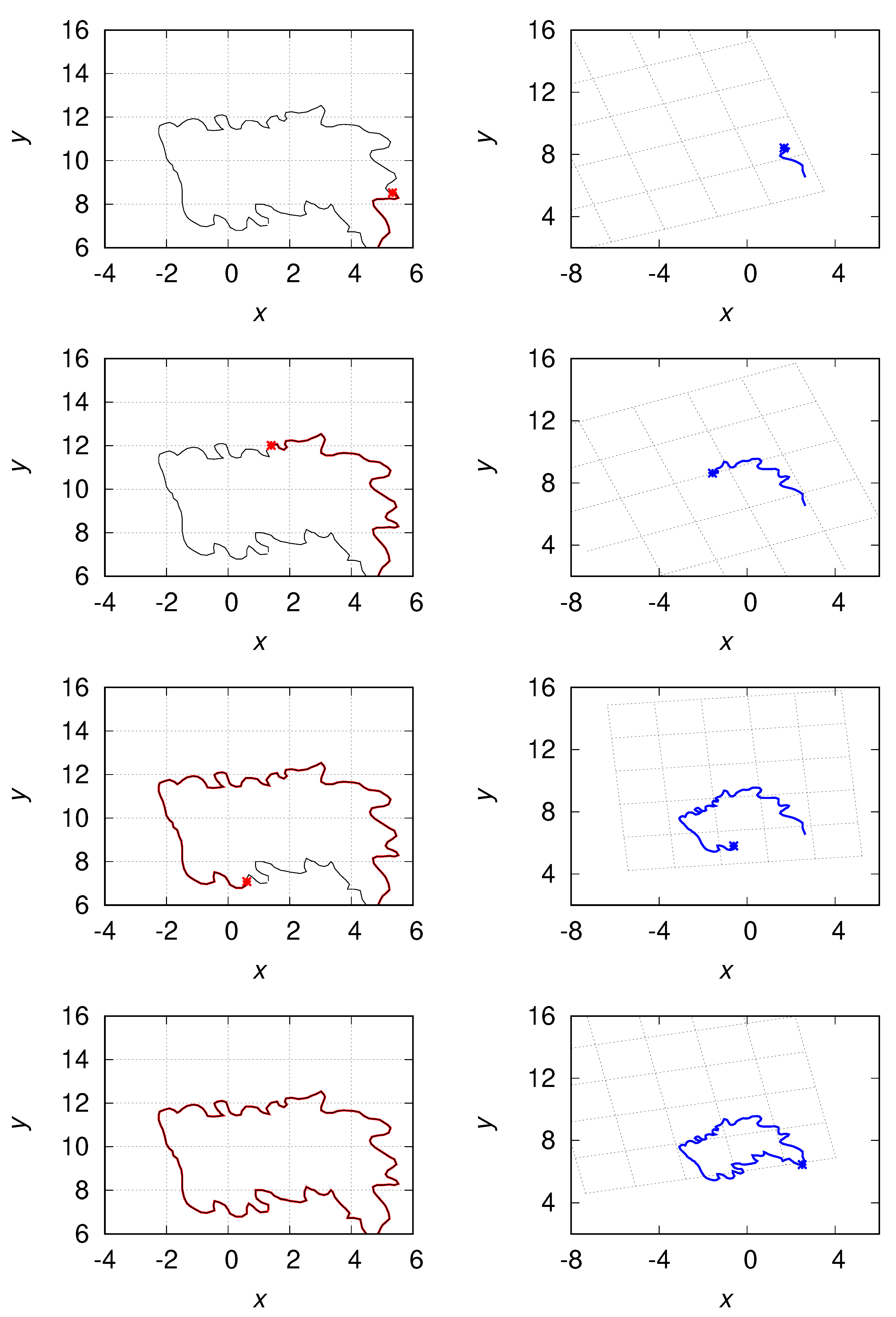
We illustrate the derived transformations with an example given in the schematic Figure 1. Let us consider an exemplary Lagrangian path of $\Phi =0$, which is, similarly as in Ref. [5] divided into small segments and parametrized. We move along the isoline, by tracking a growing tip of the curve (Figure 1, left panel) and transform it according to Equations (96) and (97) (right panel in Figure 1). Points of space $x^{\prime }$ are translated, rotated and rescaled according to Equations (105) and (106).

6. Approximate Shape of the Scalar Isolines for the Conformal Transformations of Both x and $x^{\prime }$

It was shown above that the considered set of Equations (11)–(13) and (18) are invariant under the proposed set of transformations (23)–(31). In spite of this, it is not easy to interpret these results from the physical point of view. In particular, the fact that $\mathbf{x}$ and ${\mathbf{x}}^{\prime }$ spaces transform differently. As it is evident from the example of global transformations from Section 5, the $\mathbf{x}$ space is transformed conformally according to Equations (96) and (97), whereas the ${\mathbf{x}}^{\prime }$ space is rotated and rescaled, according to Equations (105) and (106), see also Figure 1.

We argue here that the obtained transformed isoline could be interpreted as an approximation of an isoline in the conformally transformed geometry both for $\mathbf{x}$ and ${\mathbf{x}}^{\prime }$, under certain conditions. To show it let us first assume that both $\mathbf{x}$ and ${\mathbf{x}}^{\prime }$ transform conformally according to

$$\begin{array}{c}\hfill x^{*}=\mathcal{F}(x,y),y^{*}=\mathcal{G}(x,y),{x^{\prime }}^{*}=\mathcal{F}(x^{\prime },y^{\prime }),{y^{\prime }}^{*}=\mathcal{G}(x^{\prime },y^{\prime }),\end{array}$$

(112)

see also Equations (96) and (97) for the definitions of functions $\mathcal{F}$ and $\mathcal{G}$. The goal is to calculate the conditional velocities $\langle u(x,t)|\varphi ,x\rangle$ and $\langle v(x,t)|\varphi ,x\rangle$ form Equations (14) and (15) which determine the shape of the isoline. For this we assume ${\varphi }^{\prime }$ and $f_2{f}_1^{-1}$ transform according to

$$\begin{array}{cc}\hfill {\varphi }^{{}^{\prime }*}& ={\varphi }^{\prime }{\left[{\left(\frac{\partial \mathcal{F}(x^{\prime },y^{\prime })}{\partial x^{\prime }}\right)}^2+{\left(\frac{\partial \mathcal{F}(x^{\prime },y^{\prime })}{\partial y^{\prime }}\right)}^2\right]}^A={\varphi }^{\prime }{\left[\mathcal{D}(x^{\prime },y^{\prime })\right]}^{-2A},\hfill \end{array}$$

(113)

$$\begin{array}{cc}\hfill f_2^{*}{f}_1^{*-1}& =f_2{f}_1^{-1}{\left[{\left(\frac{\partial \mathcal{F}(x^{\prime },y^{\prime })}{\partial x^{\prime }}\right)}^2+{\left(\frac{\partial \mathcal{F}(x^{\prime },y^{\prime })}{\partial y^{\prime }}\right)}^2\right]}^{-A}=f_2{f}_1^{-1}{\left[\mathcal{D}(x^{\prime },y^{\prime })\right]}^{2A},\hfill \end{array}$$

(114)

where A is a constant, which remains unspecified so far. With this, after calculating the determinant of the Jacobi matrix, the transformed increment $\mathrm{d}{x}^{\prime *}\mathrm{d}{y}^{\prime *}\mathrm{d}{\varphi }^{\prime *}$ present in the integrals in Equations (14) and (15) reads

$$\mathrm{d}{x}^{\prime *}\mathrm{d}{y}^{\prime *}\mathrm{d}{\varphi }^{\prime *}=\mathrm{d}{x}^{\prime }\mathrm{d}{y}^{\prime }\mathrm{d}{\varphi }^{\prime }{\left[{\left(\frac{\partial \mathcal{F}(x^{\prime },y^{\prime })}{\partial x^{\prime }}\right)}^2+{\left(\frac{\partial \mathcal{F}(x^{\prime },y^{\prime })}{\partial y^{\prime }}\right)}^2\right]}^{A+1}=\mathrm{d}{x}^{\prime }\mathrm{d}{y}^{\prime }\mathrm{d}{\varphi }^{\prime }{\left[\mathcal{D}(x^{\prime },y^{\prime })\right]}^{-2-2A}.$$

(115)

It is clear the considered set of Equations (11)–(13) and (18) is not invariant under the above set of transformations. However, we note the coefficients ${\alpha }^{\mathit{1}}$ and ${\alpha }^{\mathit{2}}$ defined in Equation (7) are singular at point $x=x^{\prime }$. This singularity means that the largest contribution to the value of the integrals in Equations (14) and (15) for transformed variables comes from points $x^{\prime *}$ which are close to $x^{*}$. Hence, we argue we can approximate transformed conditional velocities by developing the functions $\mathcal{F}{(x^{\prime },y^{\prime })}^{\prime }$ and $\mathcal{G}{(x^{\prime },y^{\prime })}^{\prime }$ in the Taylor series as follows

$$\begin{array}{cc}\hfill x^{\prime *}& \approx \underset{=x^{*}}{\underbrace{\mathcal{F}(x,y)}}+\frac{\partial \mathcal{F}(x^{\prime },y^{\prime })}{\partial x^{\prime }}{|}_{x^{\prime }=x}(x^{\prime }-x)+\frac{\partial \mathcal{F}(x^{\prime },y^{\prime })}{\partial y^{\prime }}{|}_{x^{\prime }=x}(y^{\prime }-y),\hfill \end{array}$$

(116)

$$\begin{array}{cc}\hfill y^{\prime *}& \approx \underset{=y^{*}}{\underbrace{\mathcal{G}(x,y)}}+\frac{\partial \mathcal{G}(x^{\prime },y^{\prime })}{\partial x^{\prime }}{|}_{x^{\prime }=x}(x^{\prime }-x)+\frac{\partial \mathcal{G}(x^{\prime },y^{\prime })}{\partial y^{\prime }}{|}_{x^{\prime }=x}(y^{\prime }-y).\hfill \end{array}$$

(117)

This form is already similar to the solution (105) and (106) from the previous section, apart from the scaling factor ${\mathcal{D}}^{2/3}$ which is not present here.

With this, and after some straightforward transformations, the coefficients ${\alpha }^{\mathit{1}*}$ and ${\alpha }^{\mathit{2}*}$ in Equation (7) can be approximated by

$$\begin{array}{c}\hfill {\alpha }^{\mathit{1}*}\approx {\alpha }^1(x-x^{\prime }){\left[\mathcal{D}(x,y)\right]}^m\frac{\partial \mathcal{F}(x^{\prime },y^{\prime })}{\partial x^{\prime }}{|}_{x^{\prime }=x}+{\alpha }^2(x-x^{\prime }){\left[\mathcal{D}(x,y)\right]}^m\frac{\partial \mathcal{F}(x^{\prime },y^{\prime })}{\partial y^{\prime }}{|}_{x^{\prime }=x}\end{array}$$

(118)

$$\begin{array}{c}\hfill {\alpha }^{\mathit{2}*}\approx {\alpha }^1(x-x^{\prime }){\left[\mathcal{D}(x,y)\right]}^m\frac{\partial \mathcal{G}(x^{\prime },y^{\prime })}{\partial x^{\prime }}{|}_{x^{\prime }=x}+{\alpha }^2(x-x^{\prime }){\left[\mathcal{D}(x,y)\right]}^m\frac{\partial \mathcal{G}(x^{\prime },y^{\prime })}{\partial y^{\prime }}{|}_{x^{\prime }=x},\end{array}$$

(119)

The same approximation will be used to replace the transformed increment $\mathrm{d}{x}^{\prime *}\mathrm{d}{y}^{\prime *}\mathrm{d}{\varphi }^{\prime *}$ from Equation (115) by $\mathrm{d}{x}^{\prime }\mathrm{d}{y}^{\prime }\mathrm{d}{\varphi }^{\prime }{\left[\mathcal{D}(x,y)\right]}^{-2-2A}$. With this, the transformed conditional velocities from Equations (14) and (15) read

$$\begin{array}{cc}\hfill & {\langle u(x,t)|\varphi ,x\rangle }^{*}\approx {\left[\mathcal{D}(x,y)\right]}^{-2-2A+m}\left[\frac{\mathcal{F}(x,y)}{\partial x}\langle u(x,t)|\varphi ,x\rangle +\frac{\mathcal{F}(x,y)}{\partial y}\langle v(x,t)|\varphi ,x\rangle \right],\hfill \end{array}$$

(120)

$$\begin{array}{cc}\hfill & {\langle v(x,t)|\varphi ,x\rangle }^{*}\approx {\left[\mathcal{D}(x,y)\right]}^{-2-2A+m}\left[\frac{\mathcal{G}(x,y)}{\partial x}\langle u(x,t)|\varphi ,x\rangle +\frac{\mathcal{G}(x,y)}{\partial y}\langle v(x,t)|\varphi ,x\rangle \right],\hfill \end{array}$$

(121)

and are identical to Equations (110) and (111) from the previous section provided that $-2-2A+m=0$. This means that the shape of isolines in the conformally transformed geometry for both x and $x^{\prime }$ can be very close to the shape of isolines determined by the transformations presented in Section 5.

7. Discussion

In Section 3, the CG invariance derived in Refs. [9,17] for certain 2D vorticity statistics along characteristic lines of LMN equation has been generalised to a broader class of hydrodynamic models with a parameter $m>1$, see Equations (4) and (5). The value $m=2$ corresponds to vorticity in 2D, $m=3$ describes the SQG model and $m=6$ refers to the large-scale flows in a rotating shallow fluid. Invariance of scalar isolines in such model was investigated in Ref. [18], based on numerical data analysis. Derivations presented here concern analogous problem of zero-scalar characteristic lines and provide analytical confirmation of the CG invariance, under certain conditions.

Further, in Section 4, non-zero viscosity and friction were included in the analysis. It was found that the viscosity breaks the CG (apart from the case $m=8$), while equations with zero viscosity, but non-zero large-scale friction are still conformally invariant. This directly explains CG invariance in the inverse cascade, as observed in Refs. [5,6]. When energy is pumped into the system at a certain forcing scale (certain wavenumber), the double-cascade scenario occurs in 2D flows, as found in the seminal work by R. Kraichnan [25]. The energy is transported in the inverse cascade towards large scales and finally extracted by the large-scale friction. On the other hand, the direct enstrophy cascade takes place between the forcing scale and the small, Kolmogorov’s eddies were enstrophy dissipation due to viscosity takes place. Our study, which shows breaking of CG by the viscous term, could explain why the conformal invariance was not observed at small scales in Refs. [5,6].

In Section 5 explicit, global forms of the transformed quantities were derived. It was shown that the x space is transformed conformally while the $x^{\prime }$ space, needed to calculate two-point statistics in the integrals (14), (15), was translated, rotated and rescaled, see Figure 1. To interpret this result, we showed in Section 6 that the transformed characteristic isolines could be understood as approximation of isolines in conformally transformed geometry for both x and $x^{\prime }$, under certain conditions. We argued, due to the singular nature of functions ${\alpha }^{\mathit{1}}$ and ${\alpha }^{\mathit{2}}$ defined in Equation (7), the most significant contribution to the value of integral (14), (15) comes from points $x^{\prime }$ close to x. Hence, we proposed to replace the functions $\mathcal{F}(x^{\prime },y^{\prime })$ and $\mathcal{G}(x^{\prime },y^{\prime })$, see Equations (112) in the transformed integral by their Taylor series expansions (116) and (117). With this, the conditional velocities (120), (121) which determine the shape of the zero-scalar characteristic were approximately equal to the conditional velocities (110), (111) determined by the derived transformations. This result opens room for a further study. It should be validated, based on numerical data, whether the assumed approximation is good enough and how the exact zero-vorticity characteristics in the conformally-transformed flow will deviate from the result (120) and (121).

Finally, we note the obtained analytical results hold irrespective of the value of the friction coefficient $\gamma$ in Equation (1). There is numerical and experimental evidence that this coefficient affects the scaling of energy spectra in the direct cascade regime [26,27]. Large values of $\gamma$ result in larger deviations from the Kraichnan’s scaling [25] and, hence, are symmetry breaking. It could be that with increasing $\gamma$ and steeper energy spectrum the approximation discussed in Section 6 becomes less satisfied due to higher energy contribution of the large scales. However, as the studies in Refs. [26,27] concern forced turbulence, in order to draw conclusions about behaviour of turbulent systems, the role of forcing and its effect on CG should first be investigated.

8. Conclusions and Outlook

The results devoted to the conformal invariance of the statistics of two-dimensional turbulence were reviewed in Refs. [7,18]. The main result presented therein was that the scalar isolines in $2D$ turbulence are conformally invariant curves, provided that they are boundaries of large-scale clusters. CG invariance was not confirmed at small scales. It was hence argued that the CG is present only in the inverse cascade. A question posed in Ref. [7] was whether the conformal invariance of statistics of the zero-vorticity isolines could be explained by symmetry analysis of the underlying equations.

In the present work, we considered an analogous problem of the first equation from the infinite LMN hierarchy for the probability density function of the scalar. This equation is of hyperbolic type and can be solved by the method of characteristics. As argued in Ref. [21] analogies to the Lagrangian description of turbulence can be found here. The characteristic curves represent tracks of Lagrangian particles moving in the conditionally averaged velocity field. It can be concluded that the characteristic equations describe the average dynamics of a class of fluid particles.

As we showed in the present paper, the zero-scalar characteristic equations are CG invariant in the inviscid case. The presence of large-scale friction does not break CG. This finding could explain why in previous studies in Refs. [5,6,7] the CG was observed only at large scales. These scales are not influenced by viscosity, which breaks CG. The energy transfer among these scales occurs backwards, i.e., from the forcing scale towards larger structures where it is finally removed by the large-scale friction term. Even though the scalar isolines as considered in [7] are not the same objects as the characteristic lines investigated in the present paper, the mechanism which leads to the breaking or sustaining of CG is the same, due to the same underlying Equation (1).

In future studies, the analysis will be extended to arbitrary n-th equation from the infinite LMN hierarchy, such that invariance of multi-point pdf’s and multi-point statistics can be investigated. Moreover, we will add the forcing into the analysis. To include this, an extension to at least two-point statistics (second equation from the LMN hierarchy) is needed.

Finally, the results presented in Section 5 and Section 6 needs further careful studies. The first equation from the LMN hierarchy contains one-point and two-point pdf’s of the scalar. However, the latter is integrated over the variables $x^{\prime }$ and ${\varphi }^{\prime }$ and all terms in this equation are functions of x only. We showed that equation which describes evolution of the one-point pdf along zero-scalar characteristic line is conformally invariant, as the x space transforms conformally. In Section 6, we considered a different case, where both x and $x^{\prime }$ were transformed conformally. We calculated integrals which define the transformed conditional velocities using certain approximation, making use of the singular form of function under the integral. The obtained conditional velocities were, under certain conditions, identical to those derived in Section 5. Further studies are needed to find out whether and when the assumed approximation is good enough. For this, analysis of numerical data of 2D turbulence will be performed. It is also possible that similar approximation can be found in the 3D case, e.g., for flows in thin layers or for rotating fluids. There is numerical evidence that vorticity isolines are conformally invariant curves also in such case [28].