Controlling the Perturbations of Solar Radiation Pressure on the Lorentz Spacecraft

Abstract

The aim of the present paper is to analyze the viability of using Lorentz Force (LF) acting on a charged spacecraft to neutralize the effects of Solar Radiation Pressure (SRP) on the longitude of the ascending node and the argument of perigee of the spacecraft’s orbit. In this setting, the Gauss planetary equations for LF and SRP are presented and averaged over the true anomaly. The averaged variations for the longitude of the ascending node (h) and the argument of perigee (g) are invariant under the symmetry $(i,g)⟶(-i,-g)$ due to Lorentz Force. The sum of change rates due to both perturbing forces of LF and SRP is assigned by zero to estimate the charge amount to balance the variation for the argument of perigee and longitude of ascending. Numerical investigations have been developed to show the evolution of the charge quantity for different orbital parameters at both Low Earth and Geosynchronous Orbits.

1. Introduction

The importance of taking into account the influence of radiation pressure on artificial satellite motion does not admit discussion when noting the discrepancies between theories computations and practical observations of balloon-type satellites. The influence that is related to solar radiation pressure exceeds that of drag atmospheric at a height of 800 km and the force equals ${10}^{-5}$ dyn/cm² for an atmospherical model with an exospheric temperature of 1400 k [1].

Many studies are devoted to the study, analysis, and control perturbations of Solar Radiation Pressure (SRP) on the Lorentz Spacecraft (LS) from different views. In [2], the authors used the variation of vector elements approach to obtain first order relations for the change rates in the osculating elements, which are generated by SRP. In [3], the authors found first order solutions using Lagrange’s Planetary Equations (LPE). While [4] studied canonically the effect of SRP on space craft with complex shape. Furthermore, in [5], the authors studied the resonance effect, which is introduced by the commensurability between the different mean motions.

Some significant works have been performed to analyze the effect of SRP. Good examples between others are: In [1] the author discussed the effect as one of the non-gravitational force. In [6], the authors analyzed the direct effect of SRP as well as the indirect effect, which is the reflected radiation pressure of Earth or albedo effect on the spherical satellites and those of irregular forms. In [7], the authors improved a technique of propagation orbital movement in the proximity of the asteroid plane, within frame of combining the oblateness of asteroid, the SRP, and the orbit eccentricity of the asteroid about the Sun. They also used Lie transformation to eliminate the expressions, which involve inclination terms during the obtainment of required solutions. But the effect of non-sphericity and SRP are also studied within the framework of two and three bodies problem, for details see for instance [8,9,10,11,12].

In control and formation flight, the effect of SRP was also studied from different aspects, such as in [13] the authors investigated the use of SRP so as to study the formation flight condition for the limited size and power of small spacecraft. It was carried out by station keeping, pitch attitude slew, and yaw attitude slew by using reflective control devices. A nonlinear non-affine controller was also applied to give smooth control for the formation flying of small spacecraft. While in [14], the author studied the control of orbits about satellites with the effect of high eccentricity by using SRP.

Lorentz Force (LF) is used to control a spacecraft’s orbit using the magnetic fields of planets. This technique was first introduced in [15]. Since then, many applications of propellant less propulsion orbit control by using LF have been performed. For example, in [16] the authors constructed new Lorentz-augmented synchronous orbits by using the non-tilted dipole model of Earth’s magnetic field for determining the desired values of charge ratios, and realized new kinds of periapsis–synchronous and Sun–synchronous orbits. In this context, in [17] the authors studied Lorentz-augmented Jovian capture. In [18], the authors introduced millimeter-scale Lorentz propelled spacecraft. While in [19], the authors used LF to investigate the spacecraft propulsion concept for Low Earth Orbit (LEO) formation flying. They used formation configuration of triangular spacecraft to simulate and validate the merits and demerits of the proposed concept. They also showed that simple formation maneuvers can be performed solely using Lorentz Force.

The LF within the frame of a circular relative motion, which is used for flying and rendezvous around maneuvers is analyzed by [20]. In [21], the authors found the dynamical system of Lagrange’s Planetary Equations (LPE) for spacecraft motion, which is subject to the perturbation of LF, where this force is created from the charge gained on spacecraft surface electrostatically, during its motion in the magnetic fields of planets. This system is constructed by employing LF as perturbations on Kepler orbits with combining the true anomaly and inclination of orbits. They have constructed an analytical solution, which coincides with numerically-obtained result. In [22], the authors developed the dynamical system of relative motion, which is used to find analytically the approximated solutions of the charged spacecraft motion subject to the Lorentz Force. They showed that the major impact of the “Lorentz Force” on a space vehicle in a circular orbit is to change it in a track location and orbit plane. They also presented an example for rendezvous, when the spacecraft has a specified charge.

The main contributions in the aforementioned works studied mainly the applications of charged spacecraft in the magnetic fields of planets. While in [23], the authors showed the probability of using Lorentz Forces as tools for satellites’ attitude control on charged spacecrafts during their motion in magnetic fields. Furthermore, they found that the attitude motion equations of a spacecraft, analyzed its stability motion, and presented the attitude control technique by using the LF. A fault–tolerant magneto-Coulombic satellite attitude control is proposed by using charged shells. Two pairs of these shells are used for the three axes attitude stabilization of a satellite, when one of these pairs along any Earth axis fails [24].

Practical results of charged satellites such as the SCATHA and Cluster satellite showed the ability of the use of emitting electrons or ions in the process of orbit control [25,26], yet the question of how to build up a desired is still under investigation. In [15], the authors claimed that the maximum charge quantity, which can be created by recent technology is 0.03 C/kg, however numerous of the articles studying the use of LF for orbit control required charging levels that exceed ${10}^{-2}$ C/kg.

Hence, this property directed us to search for a more appropriate approach and use of Lorentz Forces. We then directed our efforts to the relative orbit control of spacecraft formation in Earth orbit. Lorentz Force is also used to eliminate the perturbation impact of the solar radiation pressure, which demands a low-charging level that is smaller than ${10}^{-2}$ C/kg.

This work includes eight sections: A literature review of controlling the perturbations of solar radiation pressure on the Lorentz spacecraft is covered in Section 1. In Section 2, the Gauss planetary equations are recalled. In Section 3, orbital averaged properties are presented while the effect of solar radiation pressure and Lorentz Force are discussed in Section 4 and Section 5, respectively. In Section 6, the values of charge per mass unit to balance the variations on the longitude of the ascending node and the argument of perigee are found as functions in the orbital elements. Section 7 is devoted to address the numerical results. Finally, the conclusion section is stated for illustrating the results graphically for Low Earth and Geosynchronous Orbits.

2. Perturbations in Orbital Elements

Let the elements of the Kepler orbit of the spacecraft be a, e, i, h, g, and l in their usual notations. In addition, n is the mean motion and r is the polar radial distance from Earth’s mass center. Furthermore, we impose that R, T, and W be the perturbing forces components in three directions orthogonal axes, which are called the radial, transverse, and normal component of the perturbing force. Then LPE for perturbations in the orbital elements in Gauss form are given by [27]:

$$\begin{array}{cc}\hfill {\displaystyle \frac{da}{dt}}=& {\displaystyle \frac{2}{n\sqrt{1-e^2}}}\left[Resinf+T{\displaystyle \frac{p}{r}}\right]\hfill \\ \hfill {\displaystyle \frac{de}{dt}}=& {\displaystyle \frac{\sqrt{1-e^2}}{na}}\left[Rsinf+T\left(cosu+cosf\right)\right]\hfill \\ \hfill {\displaystyle \frac{dI}{dt}}=& {\displaystyle \frac{1}{na\sqrt{1-e^2}}}W{\displaystyle \frac{r}{a}}cos(\omega +f)\hfill \\ \hfill {\displaystyle \frac{d\mathsf{\Omega }}{dt}}=& {\displaystyle \frac{1}{nasinI\sqrt{1-e^2}}}W{\displaystyle \frac{r}{a}}sin(\omega +f)\hfill \\ \hfill {\displaystyle \frac{d\tilde{\omega }}{dt}}=& T_a+2{sin}^2{\displaystyle \frac{1}{2}}I{\displaystyle \frac{d\mathsf{\Omega }}{dt}}\hfill \\ \hfill {\displaystyle \frac{dϵ}{dt}}=& T_b+2\sqrt{(1-e^2)}{sin}^2{\displaystyle \frac{1}{2}}I{\displaystyle \frac{d\mathsf{\Omega }}{dt}}\hfill \end{array}$$

(1)

where

$$\begin{array}{cc}\hfill T_a=& {\displaystyle \frac{\sqrt{1-e^2}}{nae}}\left[T\left(1+{\displaystyle \frac{r}{p}}\right)sinf-Rcosf\right]\hfill \\ \hfill T_b=& {\displaystyle \frac{e^2}{1+\sqrt{1-e^2}}}{\displaystyle \frac{d\tilde{\omega }}{dt}}-{\displaystyle \frac{2r}{n{a}^2}}R\hfill \end{array}$$

and $cosu=(e+cosf)/(1+ecosf)$, f is the true anomaly, $r=p/(1+ecosf)$, $p=a(1-e^2)$ is the semiilatus rectum, $\hslash =\sqrt{\mu p}$ is the constant of angular momentum, and $\mu$ is the gravitational parameter. Further orbital elements are defined by:

• a is the semi–major axis;
• e is the eccentricity;
• I is the inclination;
• $\mathsf{\Omega }$ is the longitude of ascending node;
• $\tilde{\omega }$ is the longitude of the perigee;
• $ϵ$ is the mean longitude at epoch.

The above equations are first constructed by Gauss and used to estimate the first order perturbation of Jupiter with respect to Pallas. Gauss also used these equations for constructing secular variation in the orbital elements. In fact the importance of these equations is extended to compute the element perturbations of comets and minor planets by numerical integration. Furthermore, it can be used in some applications to find only approximate perturbations. In order to avoid the time outside of trigonometric arguments and have more convenience with canonical equations (see [27] for details) the variables I, $\mathsf{\Omega }$, $\tilde{\omega }$, and $\epsilon$ will be replaced by i, h, g, and l respectively. We would like to refer $\tilde{\omega }=\omega +\mathsf{\Omega }$ where $\omega$ is the angular distance from the ascending node to the perigee and $l=nt+ϵ-\tilde{\omega }$. Utilizing these variables with Equation (1), we get:

$$\begin{array}{cc}\hfill {\displaystyle \frac{da}{dt}}=& {\displaystyle \frac{2}{n\sqrt{1-e^2}}}\left[Resinf+T(1-e^2){\displaystyle \frac{a}{r}}\right]\hfill \\ \hfill {\displaystyle \frac{de}{dt}}=& {\displaystyle \frac{\sqrt{1-e^2}}{na}}\left[Rsinf+T\left(cosu+cosf\right)\right]\hfill \\ \hfill {\displaystyle \frac{di}{dt}}=& {\displaystyle \frac{1}{na\sqrt{1-e^2}}}Wcos(g+f){\displaystyle \frac{r}{a}}\hfill \\ \hfill {\displaystyle \frac{dh}{dt}}=& {\displaystyle \frac{1}{nasini\sqrt{1-e^2}}}Wsin(g+f){\displaystyle \frac{r}{a}}\hfill \\ \hfill {\displaystyle \frac{dg}{dt}}=& T_a-cosi{\displaystyle \frac{dh}{dt}}\hfill \\ \hfill {\displaystyle \frac{dl}{dt}}=& n-{\displaystyle \frac{2r}{n{a}^2}}R-T_l\hfill \end{array}$$

(2)

where

$$\begin{array}{cc}\hfill T_l=& {\displaystyle \frac{\left(1-e^2\right)}{n{a}^{2}e}}\left[rT\left({\displaystyle \frac{a}{r}}+{\displaystyle \frac{1}{\left(1-e^2\right)}}\right)sinf-aRcosf\right]\hfill \end{array}$$

and here l is called the mean anomaly, and n is the mean motion.

In what follows, we will study the effect of the SRP and LF in Section 3 and Section 4. The components R, T, and W of the solar radiation pressure and Lorentz Force will be calculated. The variations of the argument of perigee and longitude of the node due to both forces will also be illustrated.

3. Orbital Averaging

The averaging is an effective and beneficial method to analyze the variational equations of orbital elements. The classical theory of averaging was primarily modified to simplify the nonlinearity of non-autonomous dynamical systems. If the dynamical system is expressed by:

$$\begin{array}{cc}\hfill & \dot{\mathsf{Ø}}=\delta \Psi (\mathsf{Ø},t)\hfill \\ \hfill & \mathsf{Ø}(0)={\mathsf{Ø}}_0\hfill \end{array}$$

(3)

where $\mathsf{Ø}\in \mathbb{M}\subset {\mathbb{R}}^n$, $\Psi (\mathsf{Ø},t)$ is $T$-periodic $(\Psi (\mathsf{Ø},t)=\Psi (\mathsf{Ø},t+T))$ and $\delta$ is a very small parameter, which may represent some physical quantity. We also denote by $\langle \mathsf{\Gamma }\rangle$ or $\overline{\mathsf{\Gamma }}$ for the averaging of $\mathsf{\Gamma }$. This averaging yields a mean value, thereby we get:

$$\langle \Psi \rangle ={\displaystyle \frac{1}{T}}{\int }_t^{t+T}\Psi (\mathsf{Ø},\tau )d\tau .$$

(4)

The main objective of averaging is eliminating the time dependence of the original dynamical system. Thus giving more simplifications for the obtained dynamical system. Although, we have to investigate under what restrictions the averaged and original dynamical system match, the averaging has a realistic meaning. Then with Equations (3) and (4), the averaged dynamical system is:

$$\dot{\overline{\mathsf{Ø}}}=\delta \Psi (\overline{\mathsf{Ø}}).$$

(5)

Since only the secular and long periodic variations affect the orbit with time, and eventually these perturbations change the orbit from its unperturbed state, we average the equations over the fast variable f (true anomaly) to keep only secular and long-period perturbations. Thereby, the application of the averaging theory on the variational equations of orbit is controlled by:

$$\langle \mathsf{\Gamma }\rangle ={\displaystyle \frac{1}{P}}{\int }_0^P\mathsf{\Gamma }df$$

(6)

where $\mathsf{\Gamma }$ is a perturbing potential and $P=2\pi /n$ is the period.

4. Effect of Solar Radiation Pressure

Solar Radiation (SR) is the expression that is used to characterize the Sun’s radiation. The exposure to this radiation is not a large issue on the Earth’s surface as the atmosphere is a protective layer. However, at a high altitude there is less of this preventive layer. Thereby we are exposed to a higher level of radiation. In astronomy, SRP is the force exerted by SR on objects within its reach. SRP is of interest in astrodynamics as it is one source of orbital perturbations. While Radiation Pressure (RP) is the pressure exerted upon any exposed surface to the radiation of electromagnetic. If it is absorbed, the pressure is the flux density of power divided by the light speed. But in the case that this radiation is completely reflected, the RP is doubled. For example, the Sun’s radiation towards the Earth has a power flux density of 1368 Watt/m², so the RP is about $4.6$ MPa (absorbed) [28].

The acceleration experienced by an object with mass m and cross-sectional area A, under the effect of SRP, when all of the solar radiation is absorbed is:

$$\mathbf{a}=-{\left({\displaystyle \frac{r_0}{r_1}}\right)}^2\mathcal{R}(\gamma )\mathbf{S}$$

(7)

where

$$\begin{array}{cc}\hfill & \mathcal{R}(\gamma )={\displaystyle \frac{A{S}_0}{m\mathcal{C}}}(1+\alpha ){cos}^2\gamma \hfill \\ \hfill & \mathbf{S}=cos\theta \mathbf{i}+cos\epsilon sin\theta \mathbf{j}+sin\epsilon sin\theta \mathbf{k}\hfill \end{array}$$

(8)

and

• $\mathcal{C}$ is the light speed;
• $r_0$ is the distance between the Earth and Sun;
• $r_1$ is the distance between the satellite and Sun;
• $\alpha$ is represents the reflection coefficient of the surface;
• $\gamma$ is an incident angle of falls ray at to the surface;
• $s_0$ is a solar constant due to the mean distance between the Earth and Sun;
• $\mathbf{S}$ is a unit vector in the direction of Satellite–Sun given in a geocentric equatorial frame;
• $\mathbf{i}$, $\mathbf{j}$ and $\mathbf{k}$ are unit vectors in the geocentric coordinates system;
• $\theta$ is the true longitude of the Sun;
• $\epsilon$ is the obliquity of ecliptic.

In addition to direct solar radiation pressure, there is an indirect radiation pressure emitted from the Earth, called Albedo, which is the measure of the diffuse reflection of solar radiation out of the total solar radiation received by Earth. It causes a small perturbing force on a satellite moving around the Earth. This perturbation decreases slightly with increasing altitude. Another indirect radiation pressure is perpendicular to the surface, related to specular reflection, that is the mirror-like reflection at the air-surface interface. We would like to refer that the components of indirect radiation pressure effects are neglected in Equations (7) and (8), see [4] for details. For simplicity, we impose that the Sun is moving in circular orbits, such that $\theta$ becomes its mean longitude. In addition the direction and distance of the satellite from the Sun are similar to those of the Earth ($r_1$ is the Earth–Sun mean distance). Hence $r_0\cong r_1$ and $\mathcal{R}(\gamma )={\mathcal{R}}_c$ is considered a constant. In this context, we also impose that $R_s$, $T_s$, and $W_s$ are the radial component, transverse, and the normal components of SRP, thereby these components will be controlled by:

$$\begin{array}{cc}\hfill R_s=& -{\mathcal{R}}_c\left[R_{s1}+R_{s2}+R_{s3}+R_{s4}+R_{s5}\right]\hfill \end{array}$$

(9a)

$$\begin{array}{cc}\hfill T_s=& -{\mathcal{R}}_c\left[T_{s1}-T_{s2}+T_{s3}-T_{s4}-T_{s5}\right]\hfill \end{array}$$

(9b)

$$\begin{array}{cc}\hfill W_s=& -{\mathcal{R}}_c\left[W_{s1}-W_{s2}+W_{s3}\right]\hfill \end{array}$$

(9c)

where

$$\begin{array}{cc}\hfill R_{s1}=& cos(g+h+\theta +f)\hfill \\ \hfill R_{s2}=& (1-c)sinhcos\theta sin(f+g)\hfill \\ \hfill R_{s3}=& (1+c_1)sinhsin\theta cos(f+g)\hfill \\ \hfill R_{s4}=& (1+c{c}_1)coshsin\theta sin(f+g)\hfill \\ \hfill R_{s5}=& s{s}_{1}sin\theta sin(f+g)\hfill \end{array}$$

(10)

$$\begin{array}{cc}\hfill T_{s1}=& sin(g+h+\theta +f)\hfill \\ \hfill T_{s2}=& (1-c)sinhcos\theta cos(f+g)\hfill \\ \hfill T_{s3}=& (1+c_1)sinhsin\theta sin(f+g)\hfill \\ \hfill T_{s4}=& (1+c{c}_1)coshsin\theta cos(f+g)\hfill \\ \hfill T_{s5}=& s{s}_{1}sin\theta cos(f+g)\hfill \end{array}$$

(11)

$$\begin{array}{cc}\hfill W_{s1}=& ssinhcos\theta \hfill \\ \hfill W_{s2}=& s{c}_{1}coshsin\theta \hfill \\ \hfill W_{s3}=& s{c}_{1}sin\theta \hfill \end{array}$$

(12)

here $s=sini$, $c=cosi$, $s_1=sin\epsilon$, and $c_1=cos\epsilon$.

Compiling Equations (10)–(12) with Equation (9), then we can evaluate the components of SRP for practical applications.

4.1. Variations of the Longitude of Ascending Node Due to Solar Radiation Pressure

The variation of h due to the SRP can be determined by substituting Equation (9c) into the fourth equation from Equation (2). Then the variation of h as a function of the variable of true anomaly f is given by:

$${\dot{h}}_R=\sqrt{{\displaystyle \frac{a}{\mu }}}{\mathcal{R}}_c\sqrt{1-e^2}K(h,\theta ,\epsilon ){\displaystyle \frac{sin(g+f)}{(1+ecosf)}}$$

(13)

where

$$K(h,\theta ,\epsilon )=sinhcos\theta -c_{1}coshsin\theta +c_{1}sin\theta$$

and with definitions in Equations (5) and (6), we can rewrite Equation (13) after taking the averaging over the true anomaly as:

$$\langle {\dot{h}}_R\rangle ={\displaystyle \frac{{\mathcal{R}}_c}{e}}\sqrt{{\displaystyle \frac{a}{\mu }}}\left(1-\sqrt{1-e^2}\right)K(h,\theta ,\epsilon )sing.$$

(14)

Equation (14) gives the averaged variation of the longitude of the node due to the force of the solar radiation pressure.

4.2. Variations of the Argument of Perigee Due to Solar Radiation Pressure

Substituting Equations (9a), (9b) into the fifth equation of Equation (2) we get the variation of g as a function of the true anomaly f in the form:

$${\dot{g}}_R=c{\dot{h}}_R+C_e\left[F_{1}cosf+\left(1+{\displaystyle \frac{1}{1+ecosf}}\right)F_{2}sinf\right]$$

(15)

where

$$C_e={\displaystyle \frac{{\mathcal{R}}_c}{e}}\sqrt{{\displaystyle \frac{a(1-e^2)}{\mu }}}$$

(16a)

$$\begin{array}{cc}\hfill F_1=& cos(f+g+h+\theta )+(1+c_1)sinhsin\theta cos(f+g)\hfill \\ & +\left[(1-c)sinhcos\theta +s{s}_{1}sin\theta +(1+c{c}_1)coshsin\theta \right]sin(f+g)\hfill \end{array}$$

(16b)

$$\begin{array}{cc}\hfill F_2=& -cos(f+g+h+\theta )-(1+c_1)sinhsin\theta sin(f+g)\hfill \\ & +\left[(1-c)sinhcos\theta +s{s}_{1}sin\theta +(1+c{c}_1)coshsin\theta \right]cos(f+g).\hfill \end{array}$$

(16c)

Substituting Equations (16a)–(16c) into Equation (15), and take averaging over the true anomaly f, we get:

$$\langle {\dot{g}}_R\rangle =c\langle {\dot{h}}_R\rangle +{\displaystyle \frac{{\mathcal{R}}_c}{e}}\sqrt{{\displaystyle \frac{a(1-e^2(}{\mu }}}\left[G_1-E{G}_2\right]$$

(17)

where

$$E={\displaystyle \frac{1}{e^2}}\left(1-\sqrt{{\displaystyle \frac{1-e}{1+e}}}-e\sqrt{{\displaystyle \frac{1-e}{1+e}}}\right)$$

(18a)

$$\begin{array}{cc}\hfill G_1=& \left[(s{s}_1+c{c}_{1}cosh)sin\theta \right]sing-csinhcos\theta sing\hfill \\ & +\left[coshcos\theta +c_{1}sinhsin\theta \right]cosg\hfill \end{array}$$

(18b)

$$\begin{array}{cc}\hfill G_2=& \left[s{s}_{1}sin\theta +(1-c)sinhcos\theta \right]sing-(1+c{c}_1)coshsin\theta sing\hfill \\ & +(1+c_1)sinhsin\theta cosg+cos(g+h+\theta ).\hfill \end{array}$$

(18c)

Utilizing Equations (18a)–(18c) with Equation (17), we can then estimate the averaged variation for the argument of perigee with respect to the force of the solar radiation pressure.

5. Effect of Lorentz Force

Following [21], the radial, $R_L$, transverse, $T_L$, and normal, $W_L$ components of LF affecting a satellite orbiting Earth with a magnetic field are given: respectively by

$$\begin{array}{cc}\hfill R_L=& {\displaystyle \frac{Bq\upsilon }{r^2}}\left[1-s^2{sin}^2(f+g)-{\displaystyle \frac{c\sqrt{\mu p}}{\upsilon r^2}}\right]\hfill \end{array}$$

(19a)

$$\begin{array}{cc}\hfill T_L=& {\displaystyle \frac{Bq\upsilon }{r^2}}\left[s^{2}sin2(f+g)+{\displaystyle \frac{ec}{\upsilon r}}\sqrt{{\displaystyle \frac{\mu }{p}}}sinf\right]\hfill \end{array}$$

(19b)

$$\begin{array}{cc}\hfill W_L=& {\displaystyle \frac{2Bqsc\upsilon }{r^2}}\left[1-{\displaystyle \frac{\sqrt{\mu p}}{\upsilon c{r}^2}}\right]sin(f+g)-{\displaystyle \frac{Bqse}{r^3}}\sqrt{{\displaystyle \frac{\mu }{p}}}sinfcos(f+g)\hfill \end{array}$$

(19c)

where

• B is the moment of magnetic dipole of planet;
• q is the charge per unit mass of satellite;
• $\upsilon$ is the planetary rotation speed.

5.1. Variations of the Longitude of Ascending Node Due to Lorentz Force

Substituting Equation (19c) into the fourth equation from Equation (2), after simplification, then the variation of h due to LF is given by:

$${\dot{h}}_L={\displaystyle \frac{Bq}{a^3}}\left[h_{L1}-h_{L2}+h_{L3}-h_{L4}+h_{L5}\right]$$

(20)

where

$$\begin{array}{cc}\hfill h_{L1}=& {\displaystyle \frac{\upsilon c}{n\sqrt{1-e^2}}}{\displaystyle \frac{a}{r}}-{\left({\displaystyle \frac{a}{r}}\right)}^3\hfill \\ \hfill h_{L2}=& {\displaystyle \frac{e}{4\left(1-e^2\right)}}{\left({\displaystyle \frac{a}{r}}\right)}^{2}cos(f+2g)\hfill \\ \hfill h_{L3}=& {\left({\displaystyle \frac{a}{r}}\right)}^{3}cos2(f+g)\hfill \\ \hfill h_{L4}=& {\displaystyle \frac{\upsilon c}{n\sqrt{1-e^2}}}{\displaystyle \frac{a}{r}}cos2(f+g)\hfill \\ \hfill h_{L5}=& {\displaystyle \frac{e}{16{\left(1-e^2\right)}^2}}{\left({\displaystyle \frac{a}{r}}\right)}^{2}cos(3f+2g).\hfill \end{array}$$

(21)

Substituting Equation (21) into Equation (20), and averaging over the true anomaly f, then the averaged of the longitude of ascending node h due to Lorentz Force is given by:

$$\langle {\dot{h}}_L\rangle =q{A}_1\left[A_2+e^{2}cos2g\right]$$

(22)

where

$$\begin{array}{cc}\hfill A_1=& {\displaystyle \frac{B}{2a^3{(1-e^2)}^3}}\hfill \\ \hfill A_2=& 2c{\left(\sqrt{1-e^2}\right)}^3{\displaystyle \frac{\upsilon }{n}}-(2+3e^2)\hfill \end{array}$$

(23)

5.2. Variations of the Argument of Perigee Due to Lorentz Force

Substituting Equations (19a), (19b) into the fifth equation from Equation (2), after simplification, then the variation of g due to LF is given by:

$${\dot{g}}_L={\displaystyle \frac{Bq}{a^3}}\left[\begin{array}{c}{g}_{L1}+g_{L2}+g_{L3}-g_{L4}+g_{L5}\hfill \\ +g_{L6}+g_{L7}-g_{L8}-g_{L9}\hfill \end{array}\right]$$

(24)

where

$$\begin{array}{cc}\hfill g_{L1}=& {\displaystyle \frac{a}{r}}\left({\displaystyle \frac{n}{2\upsilon c\sqrt{1-e^2}}}{\displaystyle \frac{a}{r}}-1\right){\displaystyle \frac{\upsilon c^2}{n\sqrt{1-e^2}}}\hfill \\ \hfill g_{L2}=& {\displaystyle \frac{3c}{2}}{\left({\displaystyle \frac{a}{r}}\right)}^3\left(1+{\displaystyle \frac{2\left(1-e^2\right)}{3e}}{\displaystyle \frac{a}{r}}cosf\right)\hfill \\ \hfill g_{L3}=& {\left({\displaystyle \frac{a}{r}}\right)}^2\sqrt{1-e^2}\left(s^2-2\right){\displaystyle \frac{\upsilon cosf}{2ne}}\hfill \end{array}$$

(25)

$$\begin{array}{cc}\hfill g_{L4}=& {\left({\displaystyle \frac{a}{r}}\right)}^2\left(1+\left(1-e^2\right){\displaystyle \frac{a}{r}}\right){\displaystyle \frac{ccos2f}{2\left(1-e^2\right)}}\hfill \\ \hfill g_{L5}=& \left({\displaystyle \frac{a}{r}}\right){\displaystyle \frac{\upsilon s^{2}cos(f+2g)}{2ne\sqrt{1-e^2}}}\hfill \\ \hfill g_{L6}=& {\left({\displaystyle \frac{a}{r}}\right)}^2\left(c{e}^2+s^2\chi \right){\displaystyle \frac{cos(f+2g)}{4e\left(1-e^2\right)}}\hfill \end{array}$$

(26)

$$\begin{array}{cc}\hfill g_{L7}=& {\displaystyle \frac{a}{r}}\left(1+{\displaystyle \frac{n\sqrt{1-e^2}}{\upsilon c}}{\left({\displaystyle \frac{a}{r}}\right)}^2\right){\displaystyle \frac{\upsilon c^{2}cos2(f+g)}{n\sqrt{1-e^2}}}\hfill \\ \hfill g_{L8}=& \left({\displaystyle \frac{a}{r}}\right){\displaystyle \frac{\upsilon s^{2}cos(3f+2g)}{2ne\sqrt{1-e^2}}}\hfill \\ \hfill g_{L9}=& {\left({\displaystyle \frac{a}{r}}\right)}^2\left(c{e}^2+3s^2\chi \right){\displaystyle \frac{cos(3f+2g)}{4e\left(1-e^2\right)}}\hfill \end{array}$$

(27)

and

$$\chi ={\displaystyle \frac{\upsilon }{n}}{\left(\sqrt{1-e^2}\right)}^3.$$

Substituting Equations (25)–(27) into Equation (24), and averaging over the true anomaly f, then the averaged of the variations of the argument of perigee g due to Lorentz force is also given by:

$$\langle {\dot{g}}_L\rangle =q{A}_1\left[B_1+B_{2}cos2g\right]$$

(28)

where

$$\begin{array}{cc}\hfill B_1=& (3s^2-4){\left(\sqrt{1-e^2}\right)}^3{\displaystyle \frac{\upsilon }{n}}+(8+7e^2)c\hfill \\ \hfill B_2=& s^2{\left(\sqrt{1-e^2}\right)}^3{\displaystyle \frac{\upsilon }{n}}-e^{2}c.\hfill \end{array}$$

(29)

From Equations (22) and (28), it is clear that the averaged of variations for longitude of ascending node (h) and argument of perigee (g) are invariant under the symmetry $(i,g)⟶(-i,-g)$ due to Lorentz Force, where $s=sini$ and $c=cosi$.

6. Balancing of Solar Radiation Pressure Effect

In this section, the variations on the elements with respect to the SRP and LF are combined to find a zero value for the variations depending on the control parameter q, which is the charge per mass unit for the spacecraft. Since we are interested only with the position of the orbit, the variations of the longitude of the node h and the argument of perigee g are the only variations considered, however any other element of the orbit can be controlled similarly.

6.1. Controlling on the Longitude of Ascending Node

Solving $\langle {\dot{h}}_R\rangle +\langle {\dot{h}}_L\rangle =0$, for the charge per mass unit q, we get the values of q in terms of the required values. The solution is:

$$q_h=-{\displaystyle \frac{A_1\langle {\dot{h}}_R\rangle }{e\left(A_2+e^{2}cos2g\right)}}$$

(30)

where $\langle {\dot{h}}_R\rangle$ is given by Equation (22) while $A_1$ and $A_2$ are given by Equation (23). However $q_h$ is the required charge value to balance the variation on h due to the solar radiation pressure.

6.2. Controlling on the Argument of Perigee

Solving $\langle {\dot{g}}_R\rangle +\langle {\dot{g}}_L\rangle =0$, for the charge q, we get the values of q in terms of the required values. The solution is:

$$q_g=-{\displaystyle \frac{A_1\langle {\dot{g}}_R\rangle }{\left(B_1+B_{2}cos2g\right)}}$$

(31)

where $\langle {\dot{g}}_R\rangle$ is given by Equation (28) while the $B_1$ and $B_2$ are given by Equation (29). Furthermore, $q_h$ is the required charge value to balance the variation on g with respect to the SRP.

7. Numerical Results

In this section, the required values of the charge per mass unit (q), to balance the variations on the longitude of ascending node (h) and the argument of perigee (g) due to the solar radiation pressure and Lorentz Force will be investigated numerically through Figure 1, Figure 2, Figure 3, Figure 4, Figure 5, Figure 6, Figure 7, Figure 8, Figure 9, Figure 10, Figure 11, Figure 12, Figure 13, Figure 14, Figure 15 and Figure 16, which is measured by the Coulomb/Kg unit. These investigations are given for showing the evaluation of the charge (q) versus different orbital parameters, both for Low Earth Orbit (LEO) and a Geosynchronous Orbit (GSO). The numerical values of the included parameters are $B=8\times {10}^6$ T km³, $\mu =\mathrm{398,600}$ km³/s², $\upsilon =\pi /12$ h⁻¹, $\epsilon =23.439°$, and $i=\pi /4$. The calculations have been estimated when the semi-major axes ($a=7100$ km) and the constant ${\mathcal{R}}_{\mathcal{C}}=9.2\times {10}^{-5}$ for Low Earth Orbit while the same quantities are ($a=\mathrm{42,160}$ km) and ${\mathcal{R}}_{\mathcal{C}}=4.2\times {10}^{-5}$ for Geosynchronous Orbit along with the true longitude of the Sun ($\theta =0$) in both two cases.

The charge per mass unit, which is required to balance the longitude of the node or the argument of perigee, is represented by a function that displays three variables of orbital elements, which are the argument of perigee (g), the longitude of node (h), and the eccentricity (e). In this regard, we estimate the charge per mass unit, when one of these elements is displayed as variable while the other two elements are taken as fixed parameters.

7.1. Results of Longitude of Ascending Node

The estimation of the charge per mass unit (q), which is required to balance the longitude of ascending node (h) of the spacecraft’s orbit will be shown numerically through multiple diagrams in Figure 1, Figure 2, Figure 3, Figure 4, Figure 5, Figure 6, Figure 7, Figure 8, Figure 9 and Figure 10. This estimation will be investigated by using Equation (30) in the following three subsections.

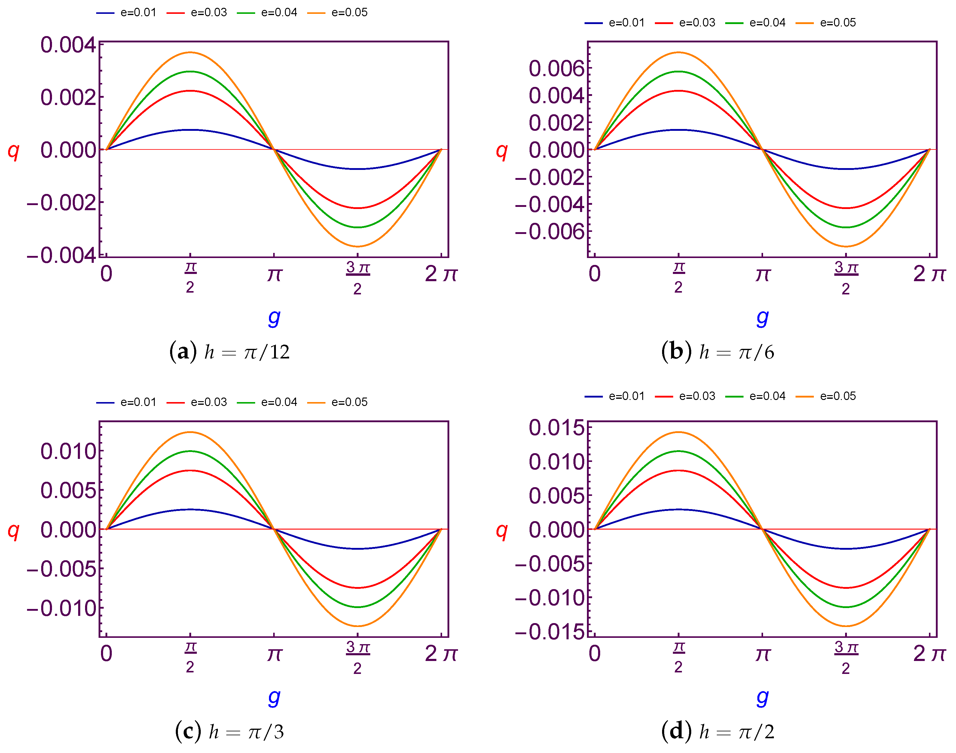
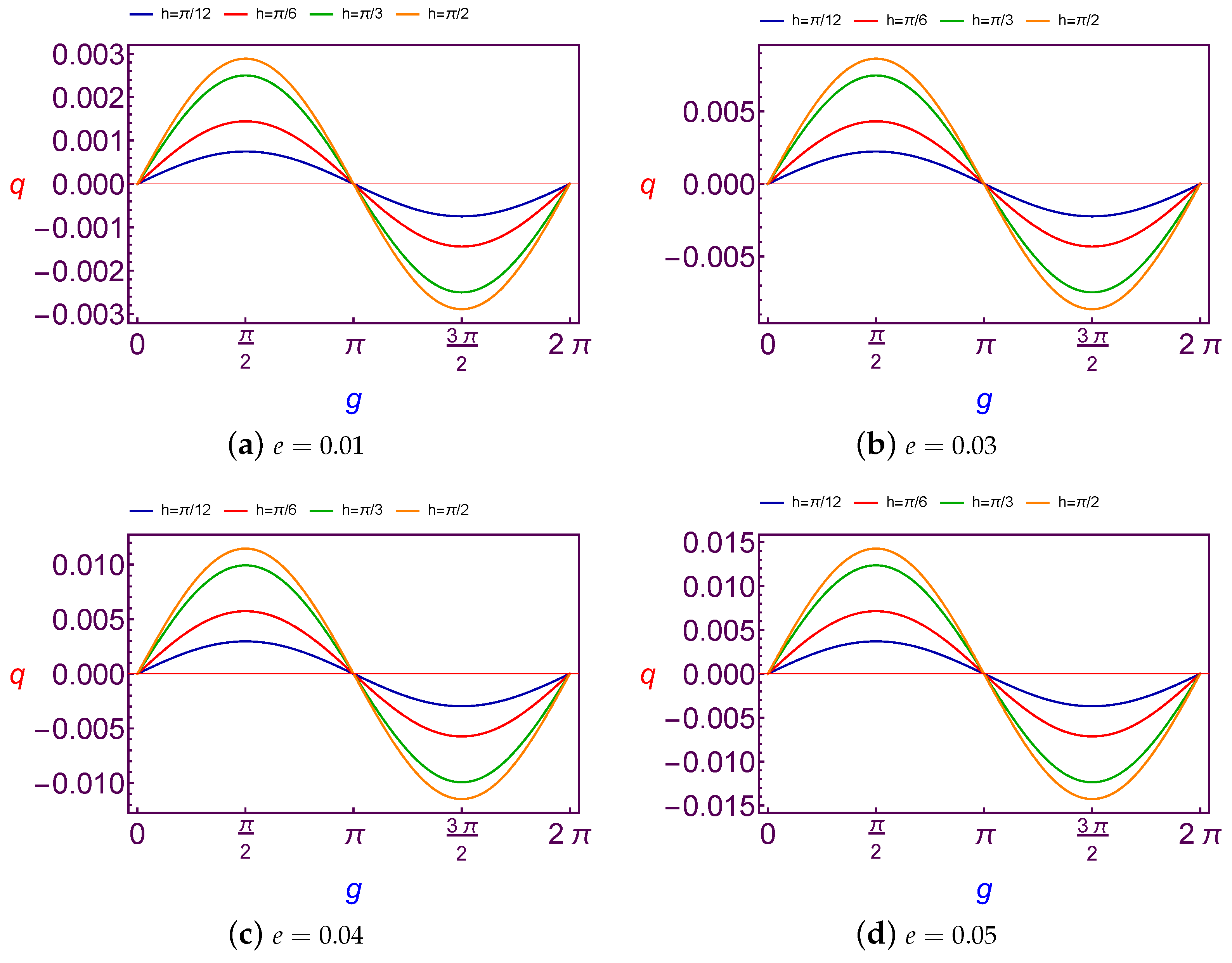
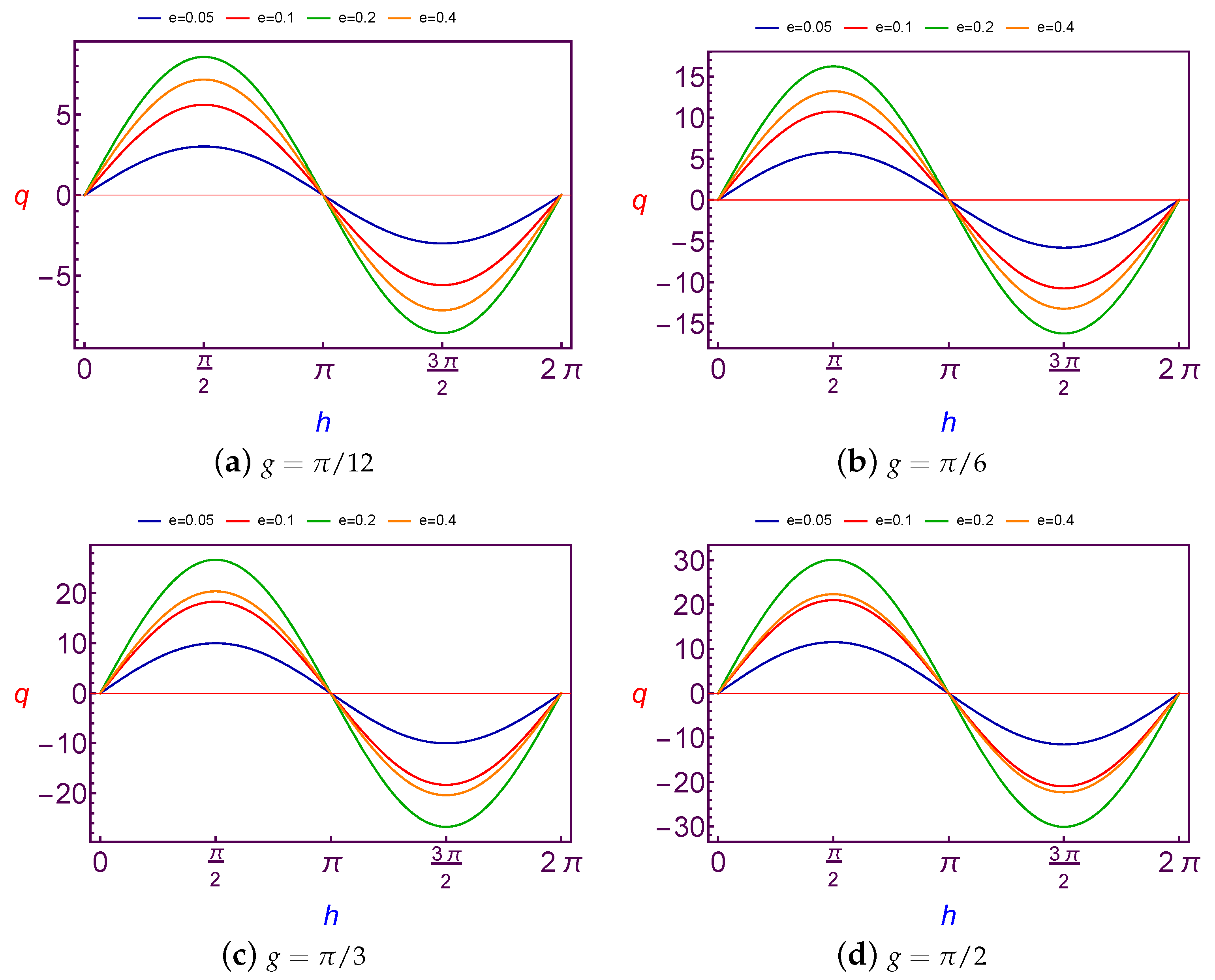
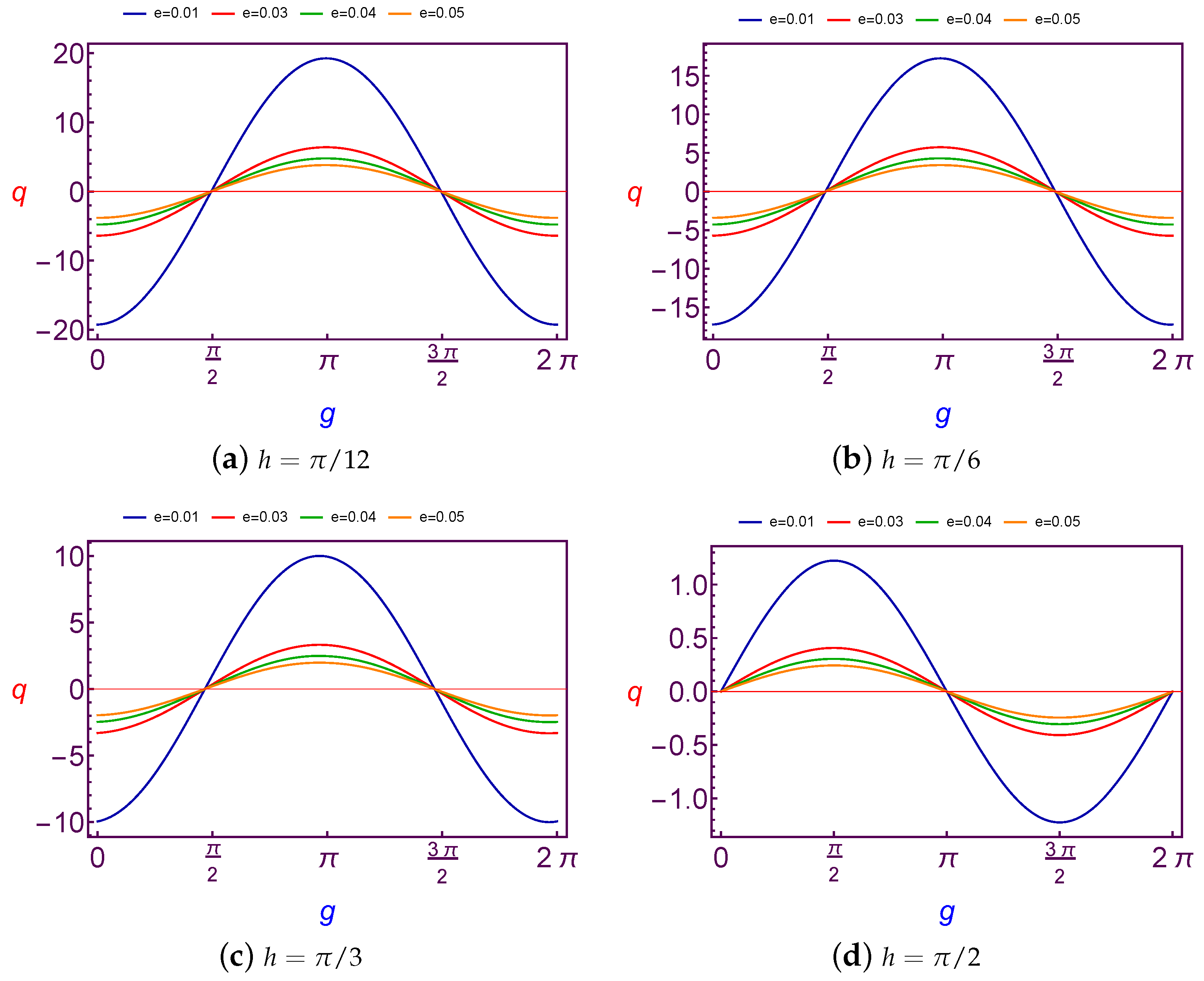
7.1.1. Evolution of Charge Quantity Versus Argument of Perigee

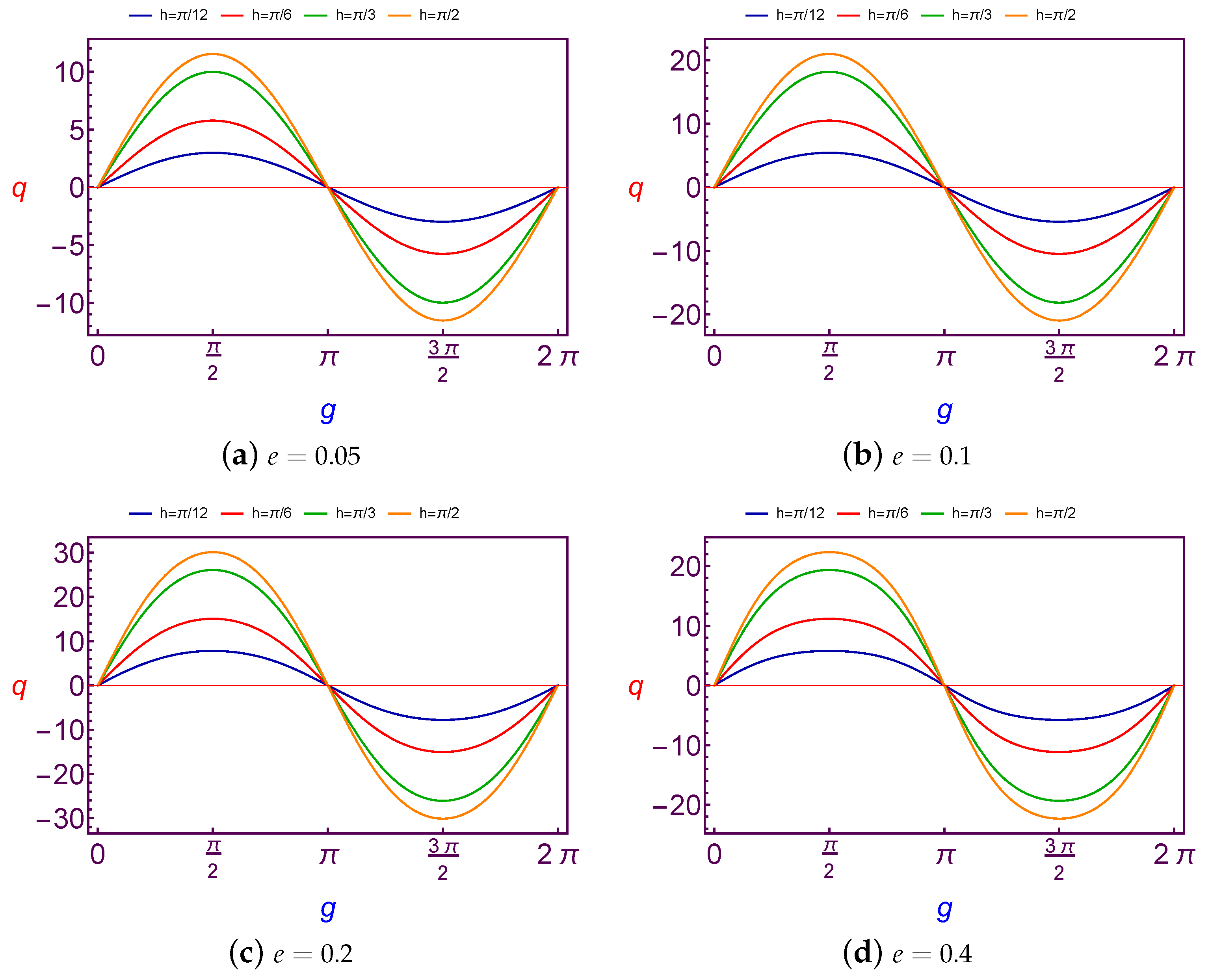
In this subsection, the required values of charge quantity is taken as a function of the argument of perigee (g). We present the computing of values for charge (q) at Low Earth Orbit in Figure 1 and Figure 2 for both different values of the longitude of ascending node (h) and the eccentricity (e), and at Geosynchronous Orbit in Figure 3 and Figure 4.

It is observed that the variation of charge values is $sine$ periodic with g. Although the amplitude changes of curves are increasing with the increase in the longitude of ascending node and eccentricity in the case of LEO. The same results are satisfied in the case of GSO too, except for that the amplitude changes of curves are fluctuating due to the changes of the eccentricity, see Figure 3.

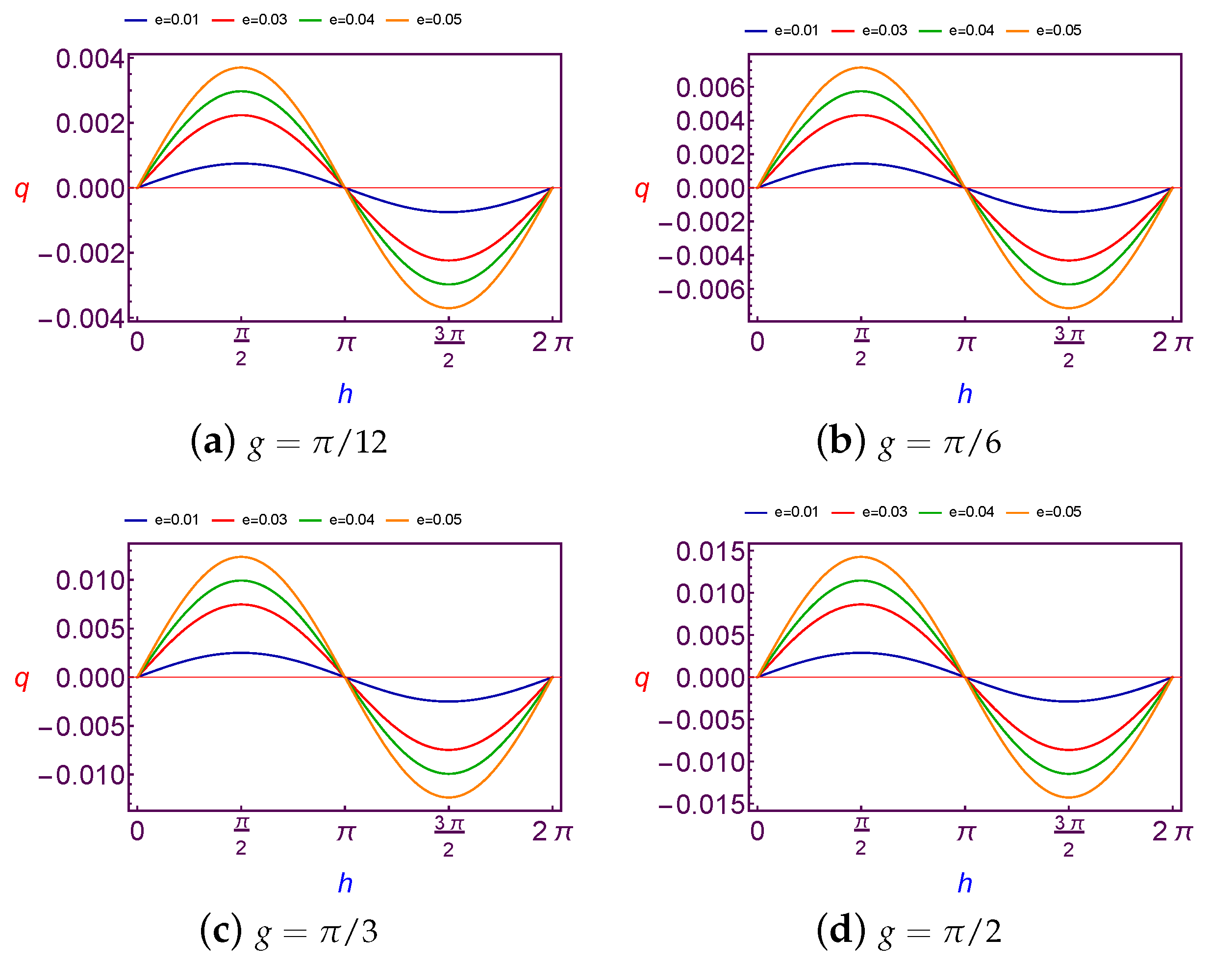
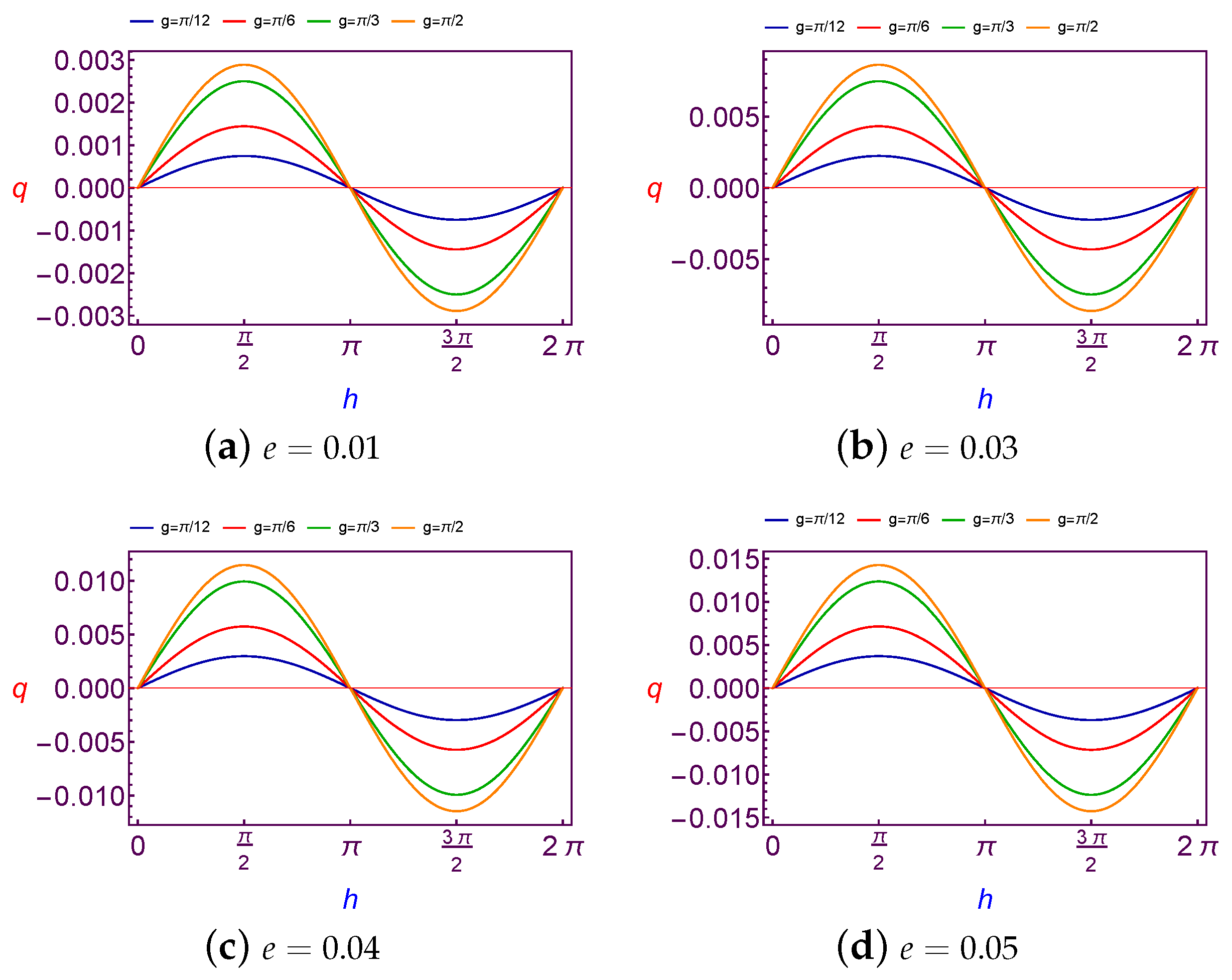
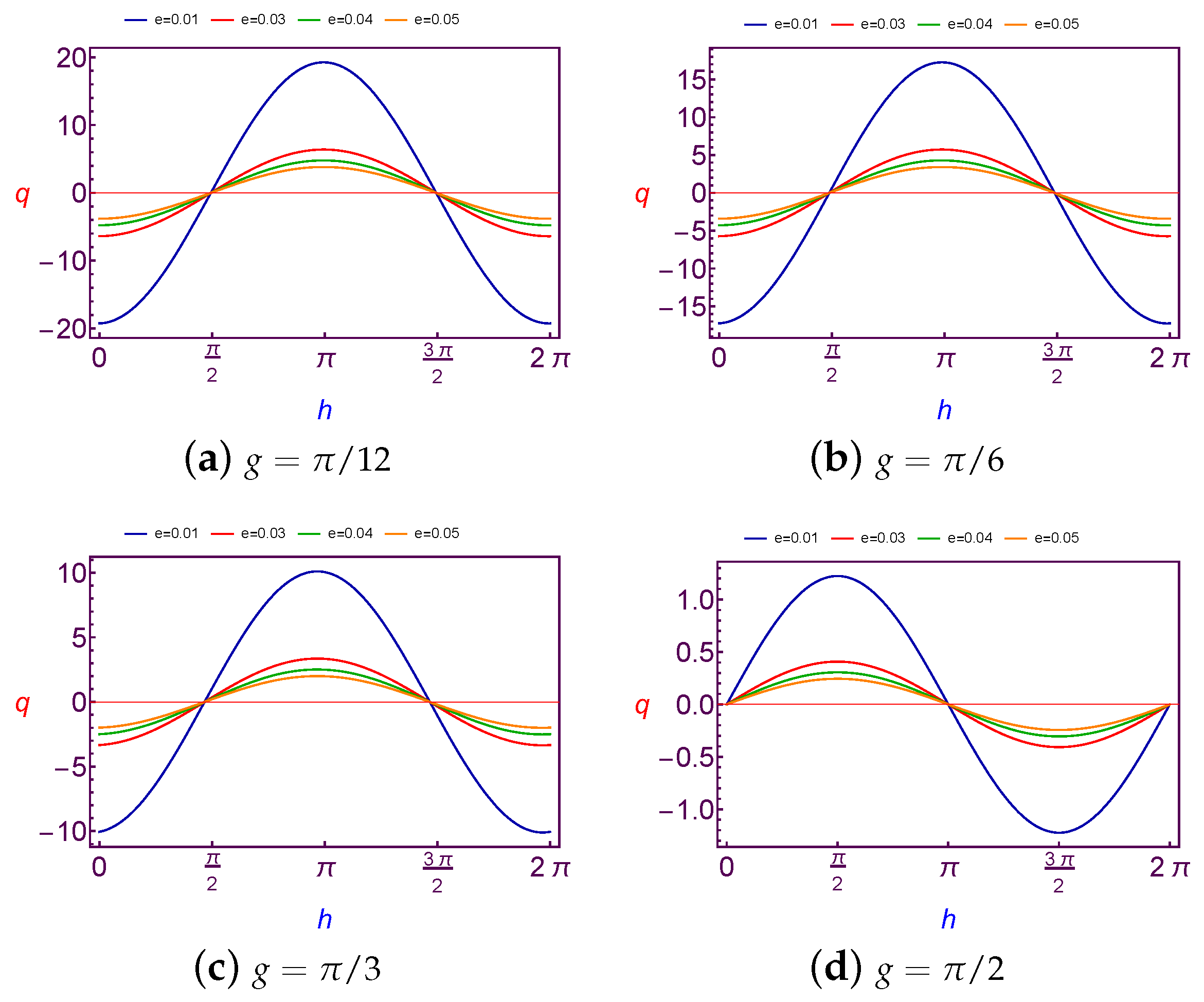
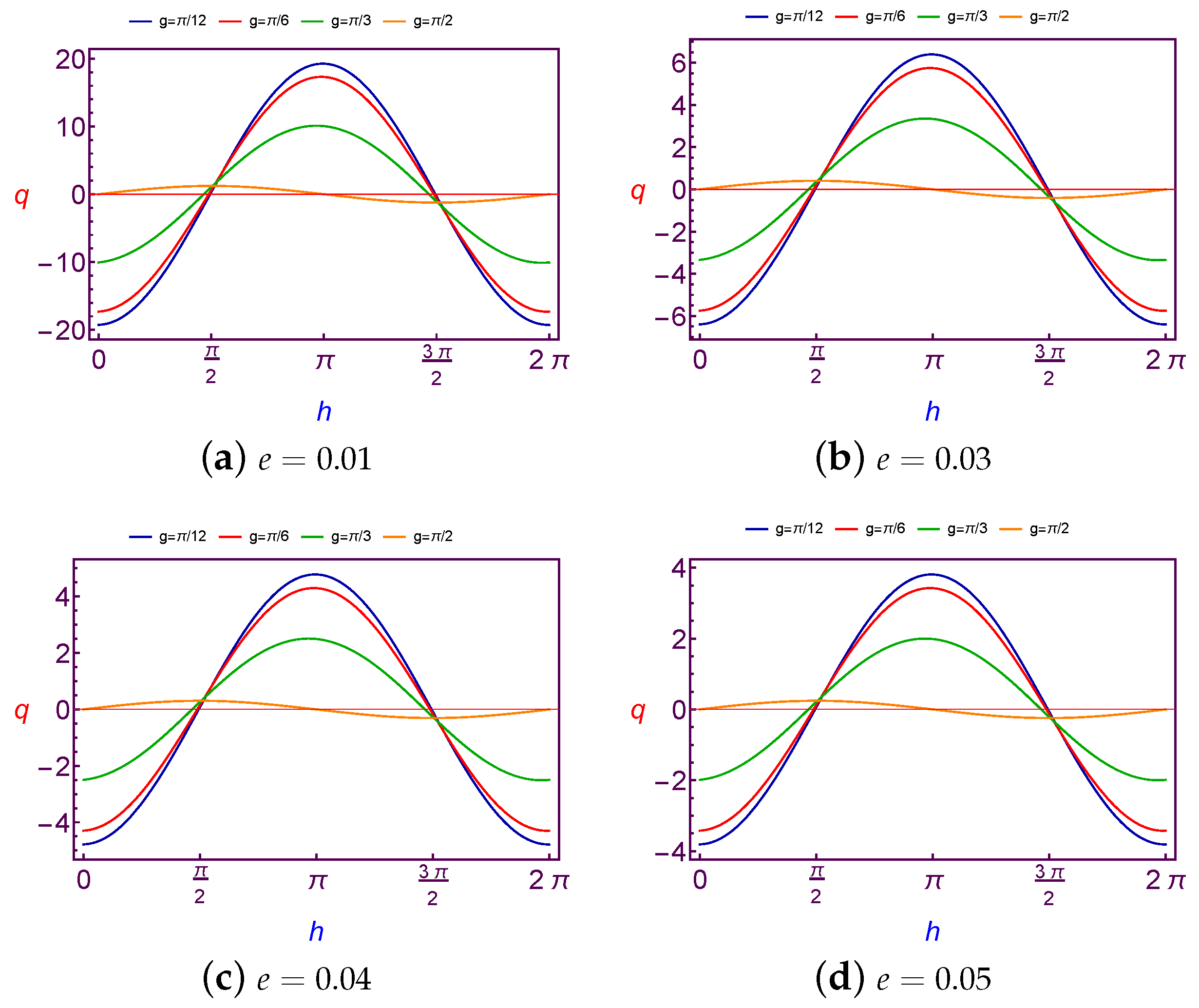
7.1.2. Evolution of Charge Quantity Versus Longitude of Ascending Node

In this subsection, the required values of charge per mass unit required to balance the longitude of ascending node is taken as a function of the longitude of ascending node (h). The values of this charge are shown at Low Earth Orbit in Figure 5 and Figure 6 for both different values of the argument of perigee (g) and the eccentricity (e), and at Geosynchronous Orbit in Figure 7 and Figure 8.

With the analysis of diagrams, we obtain a similar result as in previous sub-section, where the variation of charge values is also $sine$ periodic with h. The amplitude changes of curves are increasing with an increase in the argument of perigee and eccentricity in the case of LEO. The same results are also satisfied in the case of GSO too, except for when the amplitude changes of curves are fluctuating due to the changes of the eccentricity, see Figure 7.

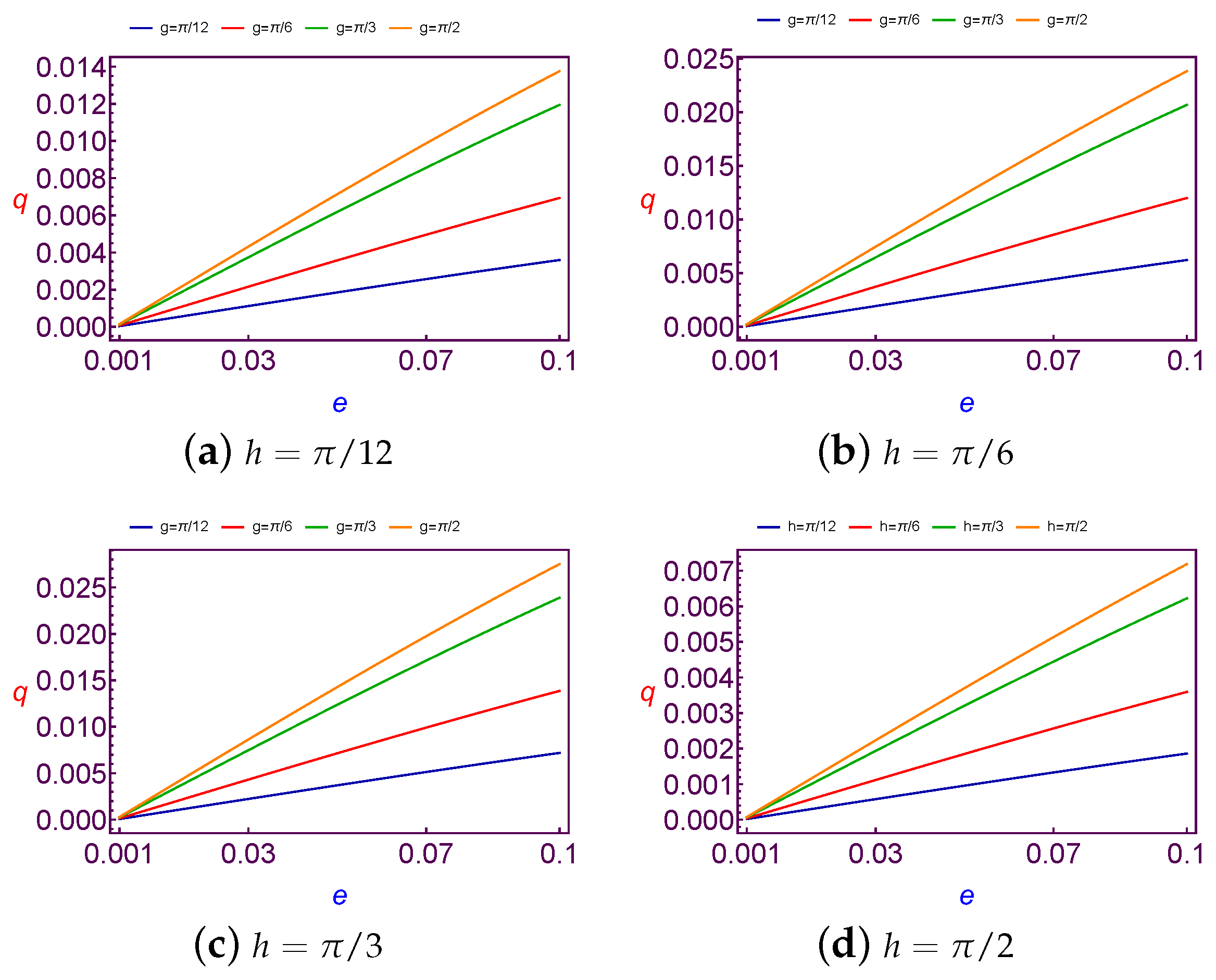
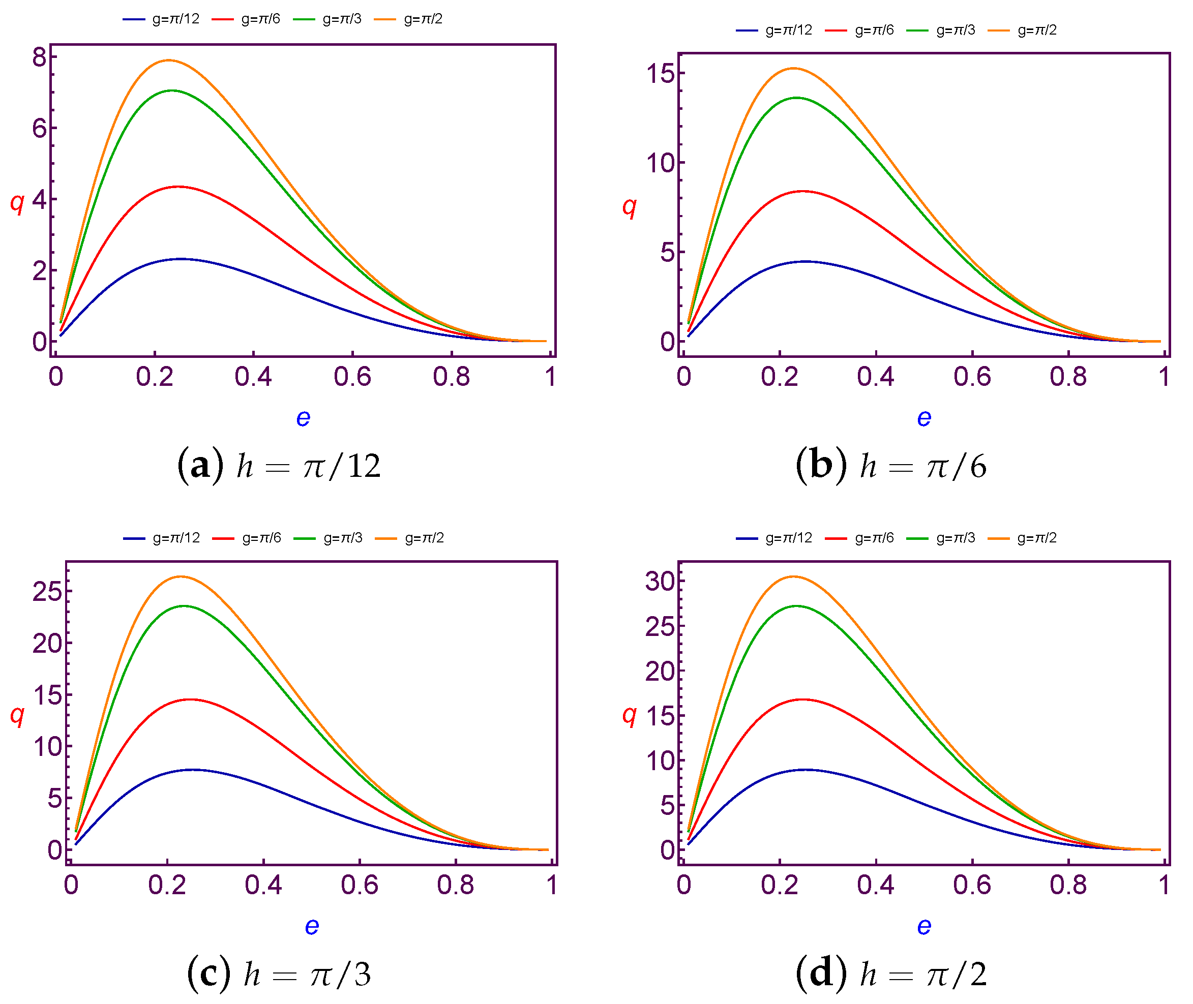
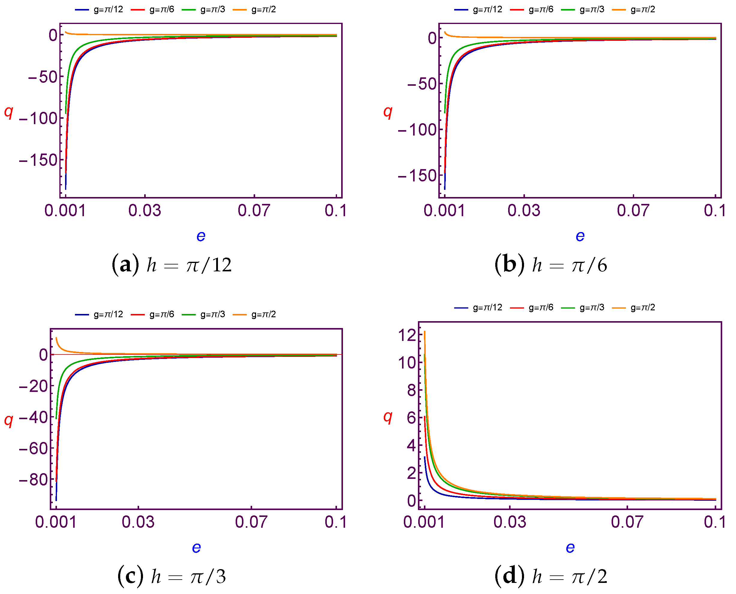
7.1.3. Evolution of Charge Quantity Versus Eccentricity

The required values of charge per mass unit required to balance the longitude of ascending node is taken as a function of the eccentricity (e). The values of this charge are shown in Figure 9 at Low Earth Orbit and at Figure 10 for both different values of the argument of perigee (g) at the fixed value of the longitude of the ascending node (h).

After analyzing these figures, we show that the variation of charge values versus the eccentricity (e) is linear for Low Earth Orbits. But in the Geosynchronous Orbit the variation of charge values versus the eccentricity (e) is nonlinearly increasing till a certain maximum (different according to different values of h and g). Then q starts to decrease with increasing e. In a simple description, the variation of the charge value may be similar to quadratic curve behavior. In addition, the same results are satisfied for both different values of the longitude of ascending node (h) at the fixed value of the argument of perigee (g).

7.2. Results of Argument of Perigee

In the following three subsections, the estimation of the charge (q), which is needed to balance the argument of perigee (g) of the spacecraft’s orbit will also be shown numerically through multiple diagrams in Figure 11, Figure 12, Figure 13, Figure 14, Figure 15 and Figure 16.

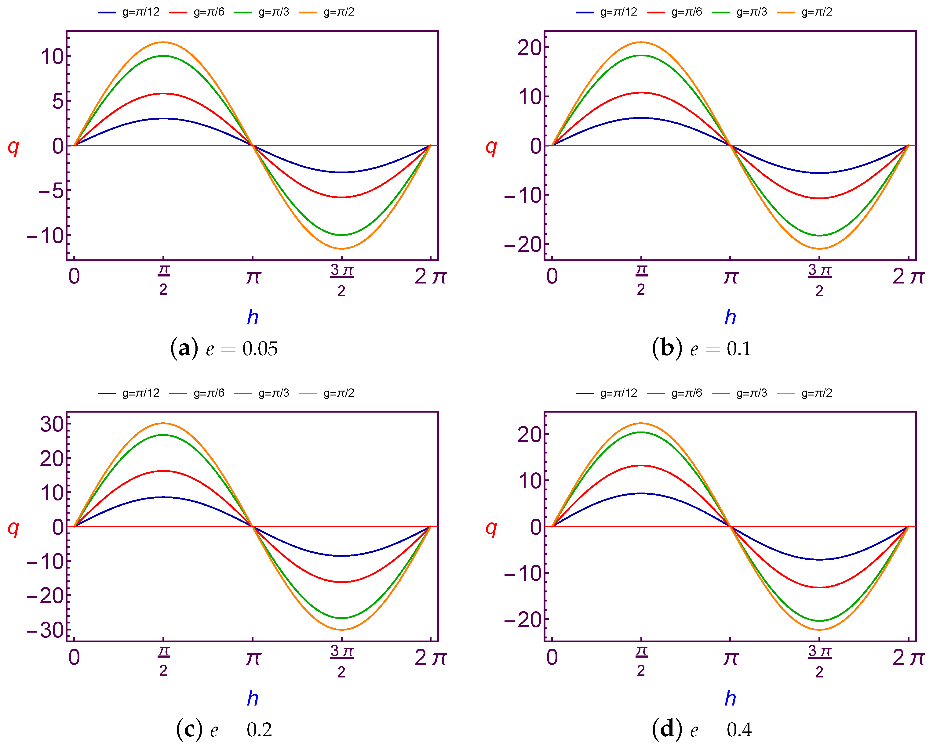
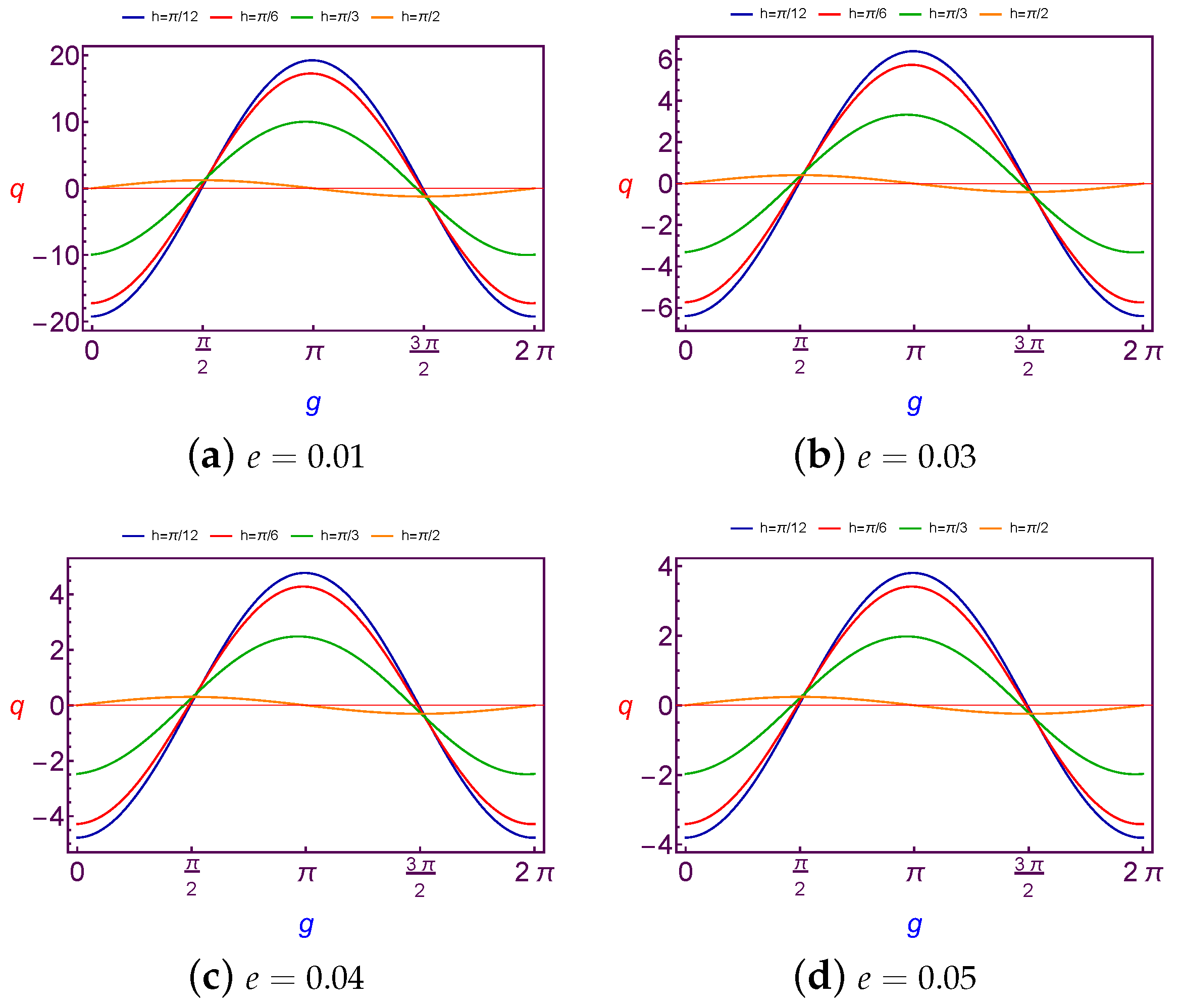
7.2.1. Evolution of Charge Quantity Versus Argument of Perigee

The required values of charge per mass unit is taken as a function of the argument of perigee (g) to balance the variation on the argument of perigee for the spacecraft’s orbit. These values will be illustrated by using Equation (31) through Figure 11 and Figure 12 in the case of Low Earth Orbits.

It is shown that the variation of charge per mass unit is $cosine$ periodic and the amplitude of the curve is decreasing with an increase in both the values of the longitude of node and eccentricity, but with a continuation in the increasing longitude of node value, the variation will be $sine$ periodic, see Figure 11d. We also emphasize that the same results are satisfied in the case of Geosynchronous Orbits.

7.2.2. Evolution of Charge Quantity Versus Longitude of Ascending Node

The charge values (q) which is needed to balance the argument of perigee (g) as a function of the longitude of perigee (h) are presented in Figure 13 and Figure 14 for Low Earth Orbit.

The obtained results here are similar to those of the previous sub-section, the variation of the required charge is $cosine$ periodic and the amplitude of the curve is decreasing with an increase in both the values of the argument of perigee and eccentricity, but with a continuation increasing in the argument of perigee value, the variation will be $sine$ periodic, see Figure 13d. The same results will satisfy the Geosynchronous Orbit.

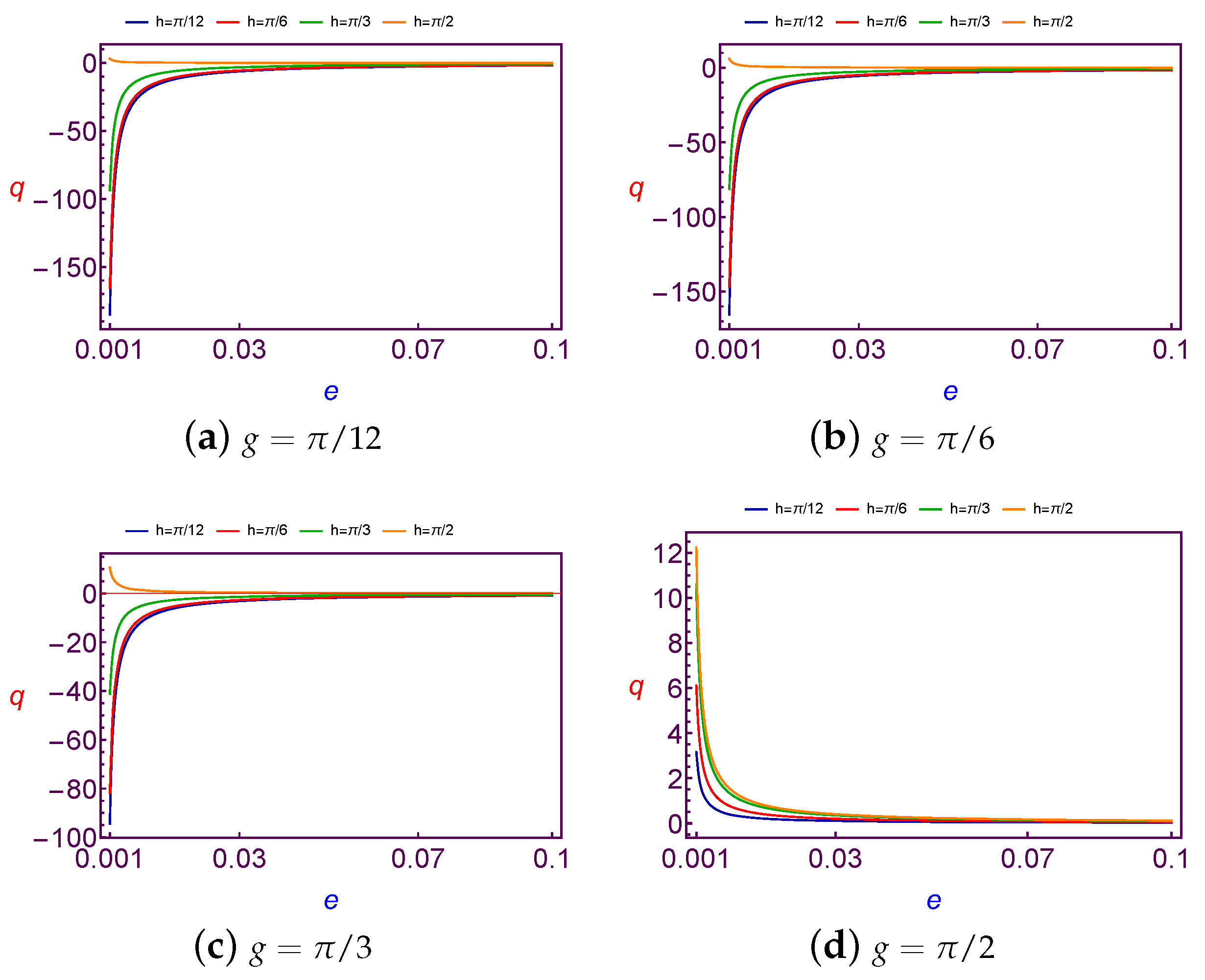
7.2.3. Evolution of Charge Quantity versus Eccentricity

The charge per mass unit values (q) required to balance the argument of perigee (g) as a function of the eccentricity e are presented in Figure 15 and Figure 16 for Low Earth Orbit.

After analyzing these figures, we demonstrate that the effect of increasing argument of perigee (g) or the longitude of node (h) is to reduce the values of the charge per mass unit (q), furthermore this value tends to zero as the eccentricity (e) tend to unity. In addition the same results are satisfied in the case of Geosynchronous Orbit, when $e\in ]0,0.1[$ in the case of Low Earth Orbit, while $e\in ]0,1[$ for Geosynchronous Orbit.

7.3. Implications on Spacecraft Attitude

In [29], the author proved that the spacecraft attitude is stimulated by three magnetic torques and subjected to a magnetic field that varies with time. These are accessible if the magnetic field and its first two time derivatives are linearly indented. Moreover, they are controllable if the magnetic field is periodic in time. Since in our study we are interested in controlling the perturbation due to solar radiation pressure, on the argument of perigee and the argument of ascending node, using LF, then the pointing of the spacecraft in the direction of the local magnetic field or the Sun is out of scope of the subject. However, it should be mentioned that controlling the Lorentz Force depends mainly on the electric charge magnitude and whether is is positive or negative, which is much easier than attitude control. In addition, solar radiation pressure effects on different orientations of the satellite can be handled with controlling the charge instead of attitude control.

A spacecraft is charged because of the fact that outer space contains high energy-charged particles, a spacecraft is naturally charged. Although these charged particles cause serious problems to the spacecraft, e.g., damage to electrical equipment and interference in measurements, but we can use them to produce electric charge that allow for the use of the Earth magnetic field and thus getting use of the Lorentz Force as an effective force in the control dynamic of the satellite whether is is orbit or attitude control. Generally, the devices that produce electric power for different uses of the satellite can also be used to charge the surface of the satellite. These devices usually have a wight of about $10\%$ of the satellite, e.g., OCEAN satellites whose electric power supply system has the weight of 584 kg, which is less than about $10\%$ of the total weight of the satellite, with a 3-year-orbital resource time [30].

8. Conclusions

In this article, a treatment was made to control the orbit position against the perturbation effect of solar radiation pressure. This was achieved through balancing the argument of perigee and longitude of ascending node of the spacecraft, by using the specific charge density (charge per mass unit). This charge was used to control the required value of Lorentz Force to provide the desired balance. The variations of the orbital elements due to both forces were calculated. The variations of g and h were set equal to zero, under the combined effect of both forces, to find the required values of the charge per mass unit q.

Multiple graphical investigations were given to illustrate the range of possible values for the charge per mass unit q, which is needed to establish the control. These investigations showed that the variation was periodic versus the argument of perigee and the longitude of ascending node in both cases of Low Earth and Geosynchronous Orbits. The obtained results also showed that for balancing the longitude of node h, the change of charge per mass unit value was periodic due to the argument of perigee g and the longitude of node with peaks varying from $1.5\times {10}^{-5}$ C/kg to $4\times {10}^{-5}$ C/kg at Low Earth Orbit, and from $5\times {10}^{-3}$ C/kg to $30\times {10}^{-3}$ C/kg at Geosynchronous Orbit.

Furthermore, the variation of charge per mass unit values required that balance of the longitude of ascending node versus the eccentricity (e) quadratic curve behavior for different values of the argument of perigee (g) and the longitude of node (h). While the same values to balance the argument of perigee were reduced with the increase in both values of h and g.

The maximum charge that can be obtained by current technology is 0.03 C/kg as mentioned in the introduction section. However, the results of the calculations show that in many cases (especially for GSO) the required charge for balancing exceeds this value. Thus we would like to remark that the graphs of high altitude at Geosynchronous Orbit show very large values for q rather than for Low Earth Orbits. This is because the Lorentz Force variations on h and g depend on ($1/a^3$), see Equations (22) and (24). Thus moving from $a=7100$ to about $\mathrm{42,160}$ means an increase by about 216 greater required values of q. In addition, the computations and graphics of the paper were produced using the latest version $12.0$ of Mathematica${}^{\circledR }$ Wolfram. Finally we emphasize that the proposed technical model is considered in the modern literature as closely related to both the electrodynamic sweeping of outer space around the Earth and the nano-electrodynamic spacecraft of future space exploration.