Structure of Neutron Stars in Massive Scalar-Tensor Gravity

 , , , and
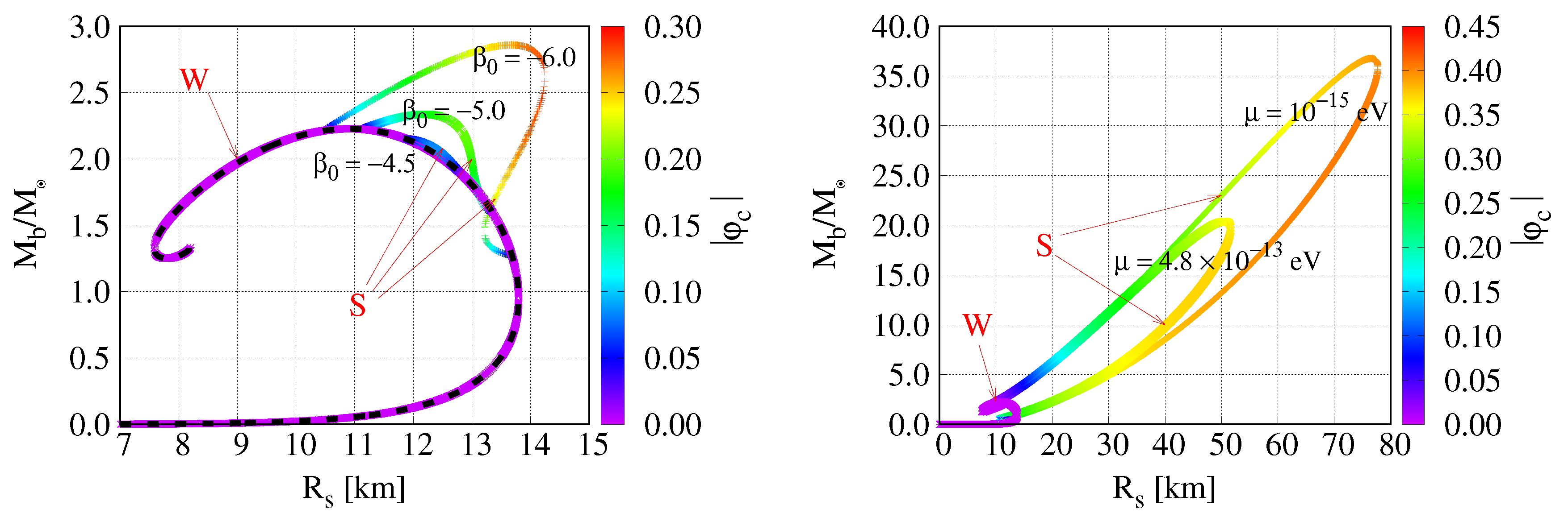
Abstract
1. Introduction
2. Formalism
- (i)
- The boundary conditions are specified at different locations of the domain, so that we have a two-point-boundary-value problem.
- (ii)
- For realistic values of the polytropic exponent , the pressure will reach zero at a finite radius ; at this point, we need to match to an exterior solution with vanishing baryon density .
- (iii)
- The asymptotic behaviour of the scalar field near infinity is determined by the scalar mass and is given byfor constants , . We are only interested in bounded solutions with . This exponential fall-off is responsible for the suppressed scalar contribution in the interaction of pulsar binaries in massive ST gravity and forms the key motivation for our study. From a purely numerical point of view, however, Equation (21) creates a significant challenge. Numerical algorithms will pick up all possible modes of a solution–even if only through roundoff error.
3. Numerical Framework
4. Results
4.1. Overall Phenomenology
4.2. Dependence on
4.3. Dependence on
4.4. Dependence on
4.5. Stability of Models
5. Conclusions
- For , the NS models of GR are also solutions of the field Equations of massive ST gravity. For , we find, additionally to the GR branch, the spontaneously scalarized class of NS solutions that Damour and Esposito-Farèse discovered in their original exploration of massless ST theory [18] and that were also identified in massive ST theory in [21]. These solutions are invariant under the scalar field transformation .
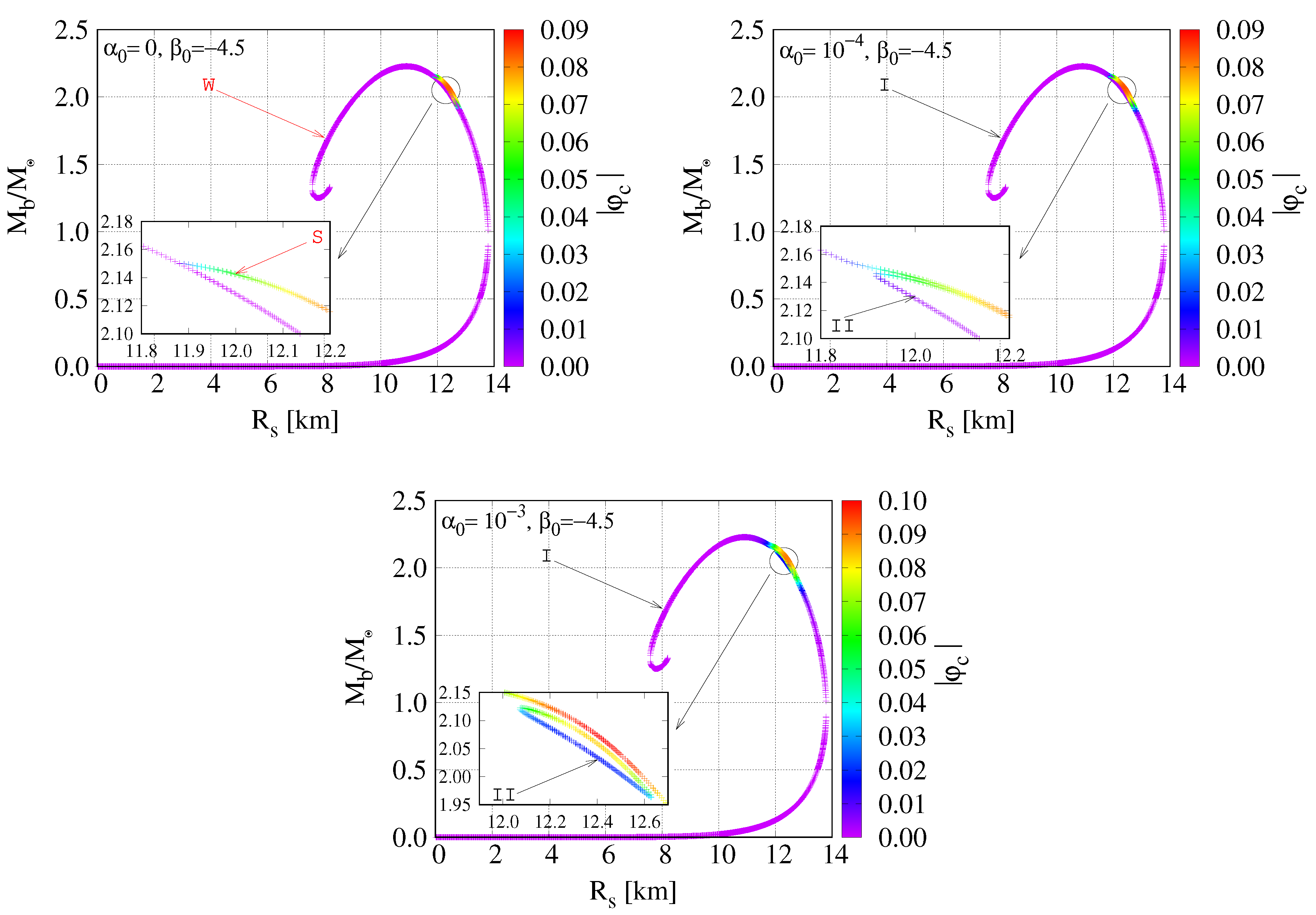
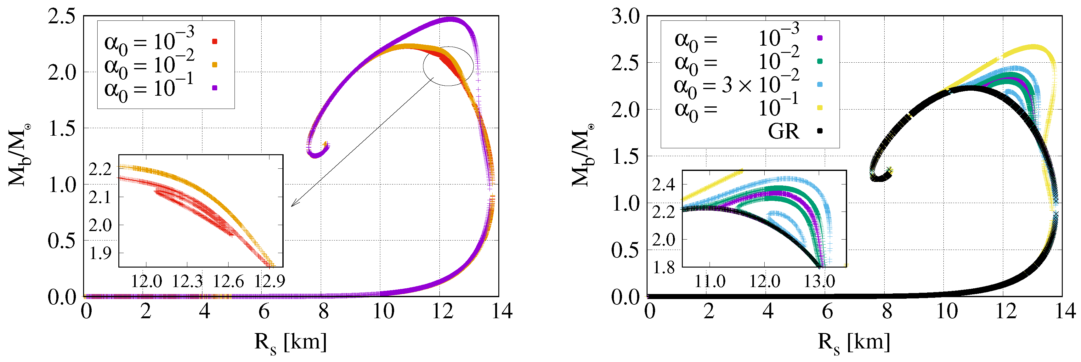
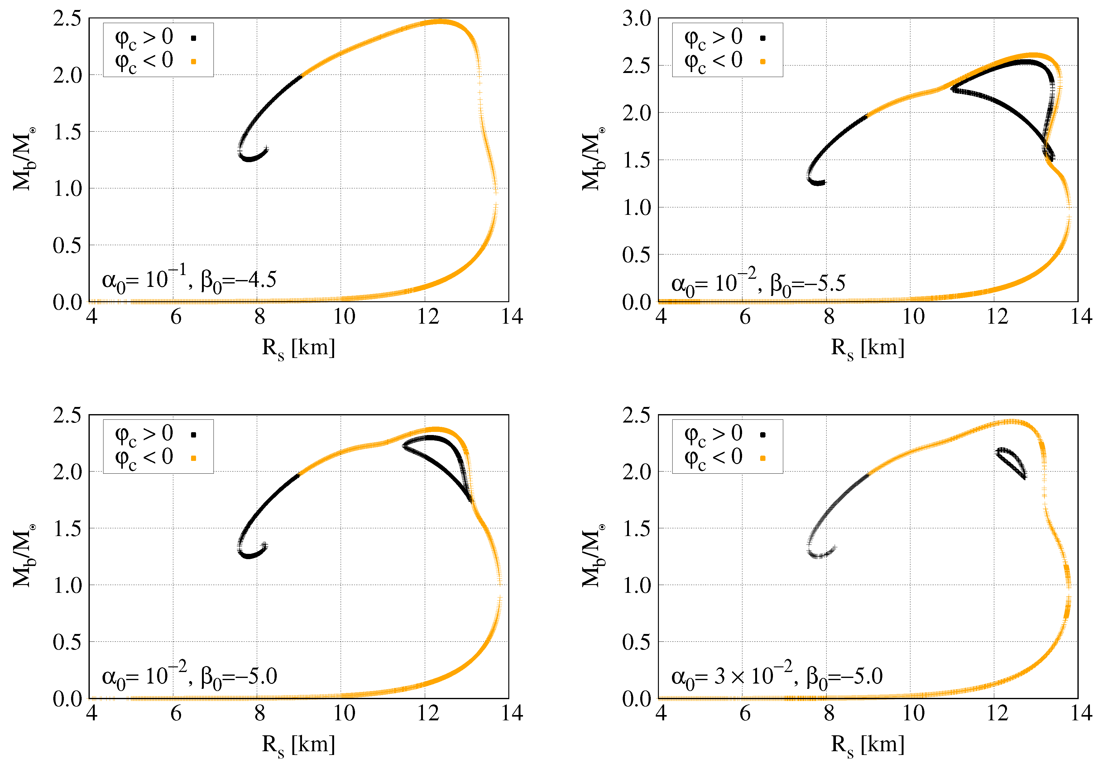
- A non-zero breaks this degeneracy and results in a dissection of the branches around the branch points; instead of the two connected branches of scalarized and non-scalarized solutions for , we now find a main branch I and a smaller loop of branch solutions; cf. Figure 2. The solutions on branches I and are characterized by different signs of the central scalar-field value ; cf. Figure 4.
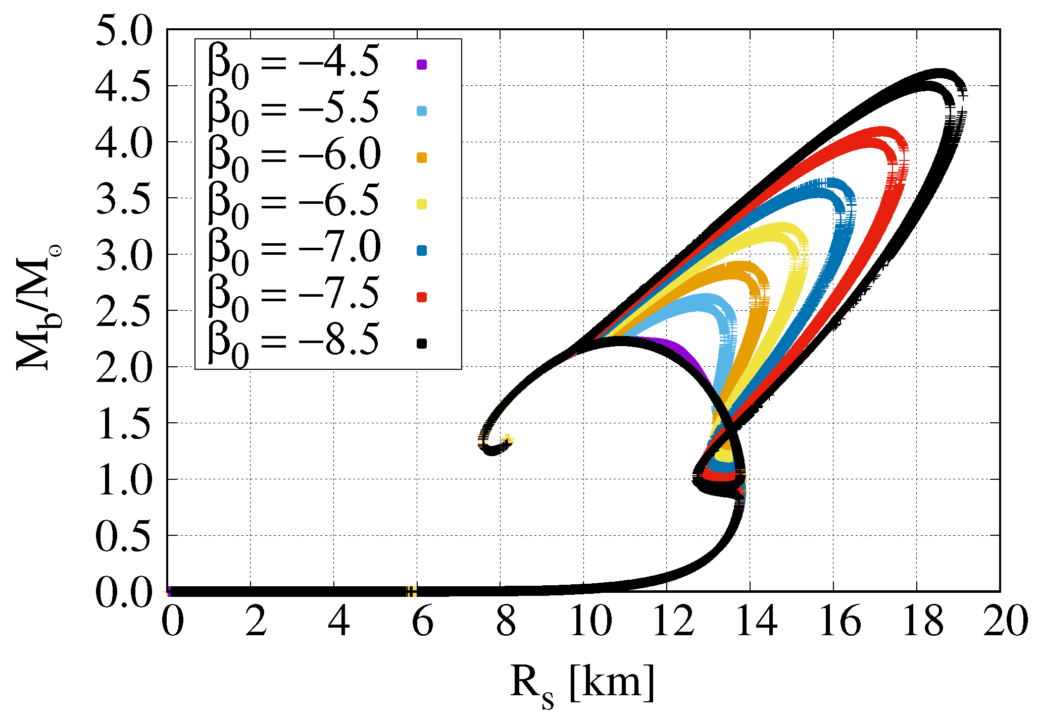
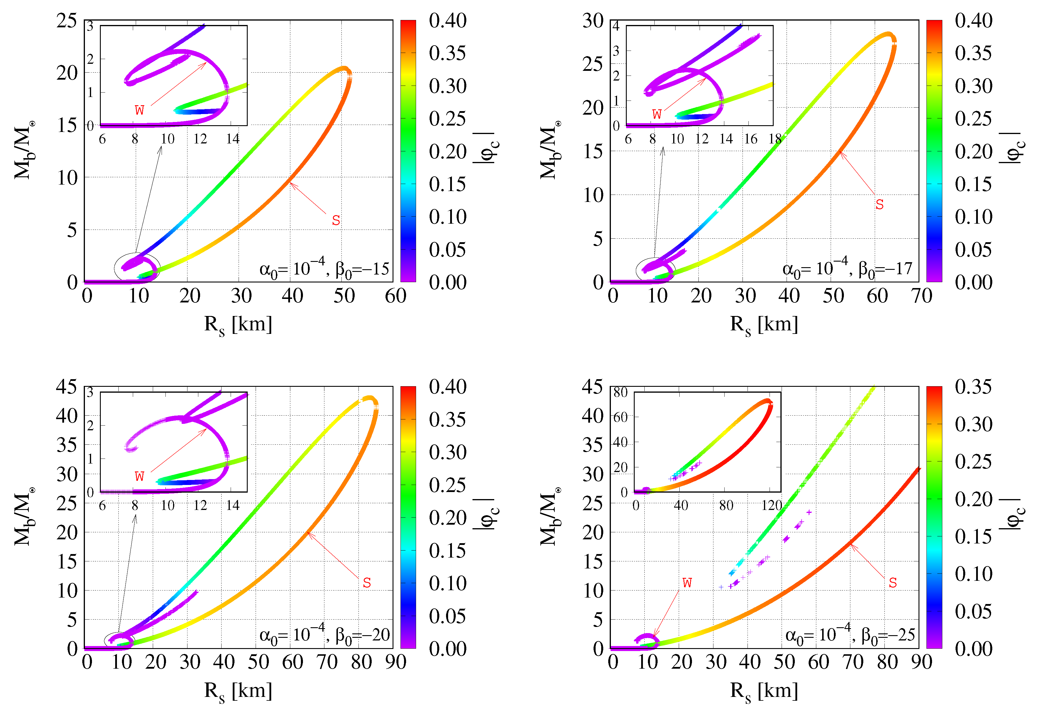
- For sufficiently negative , roughly , we observe a qualitative change in the strongly scalarized branch S of solutions. Instead of smoothly approaching the weakly scalarized branch W as happens for milder , its upper (in the sense of increasing central baryon density) tail now either crosses or completely detaches from the W branch.
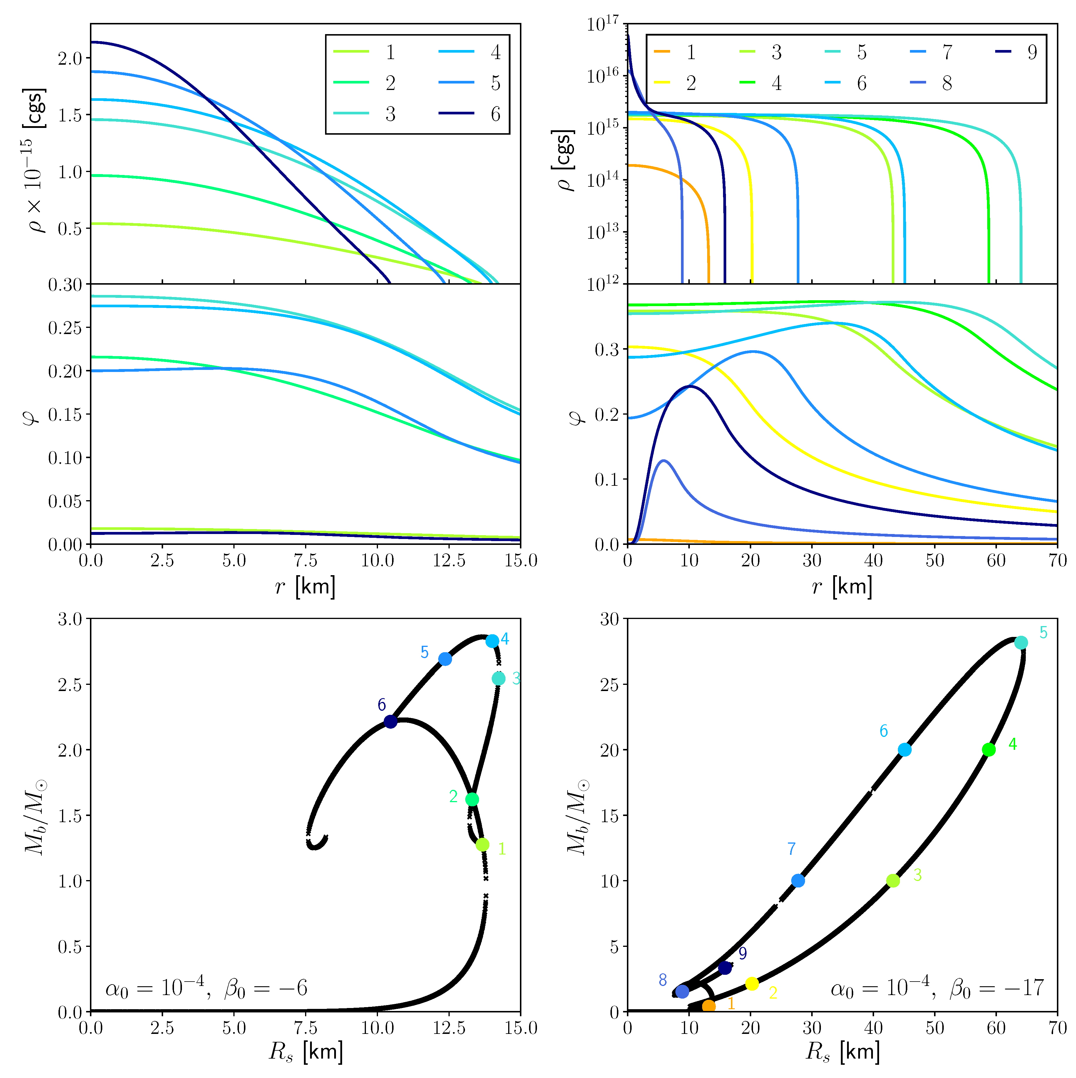
- For highly negative values of , we furthermore encounter a new type of strongly scalarized solutions at this upper end of the S branch: the maximum of the scalar field is located away from the stellar center; cf. Figure 6 and Figure 7. In its most extreme form, these solutions are composed of highly compact NS models surrounded by a scalar shell; see, e.g., [77,78] for similar “gravitational atom” like configurations in other theories of gravity.
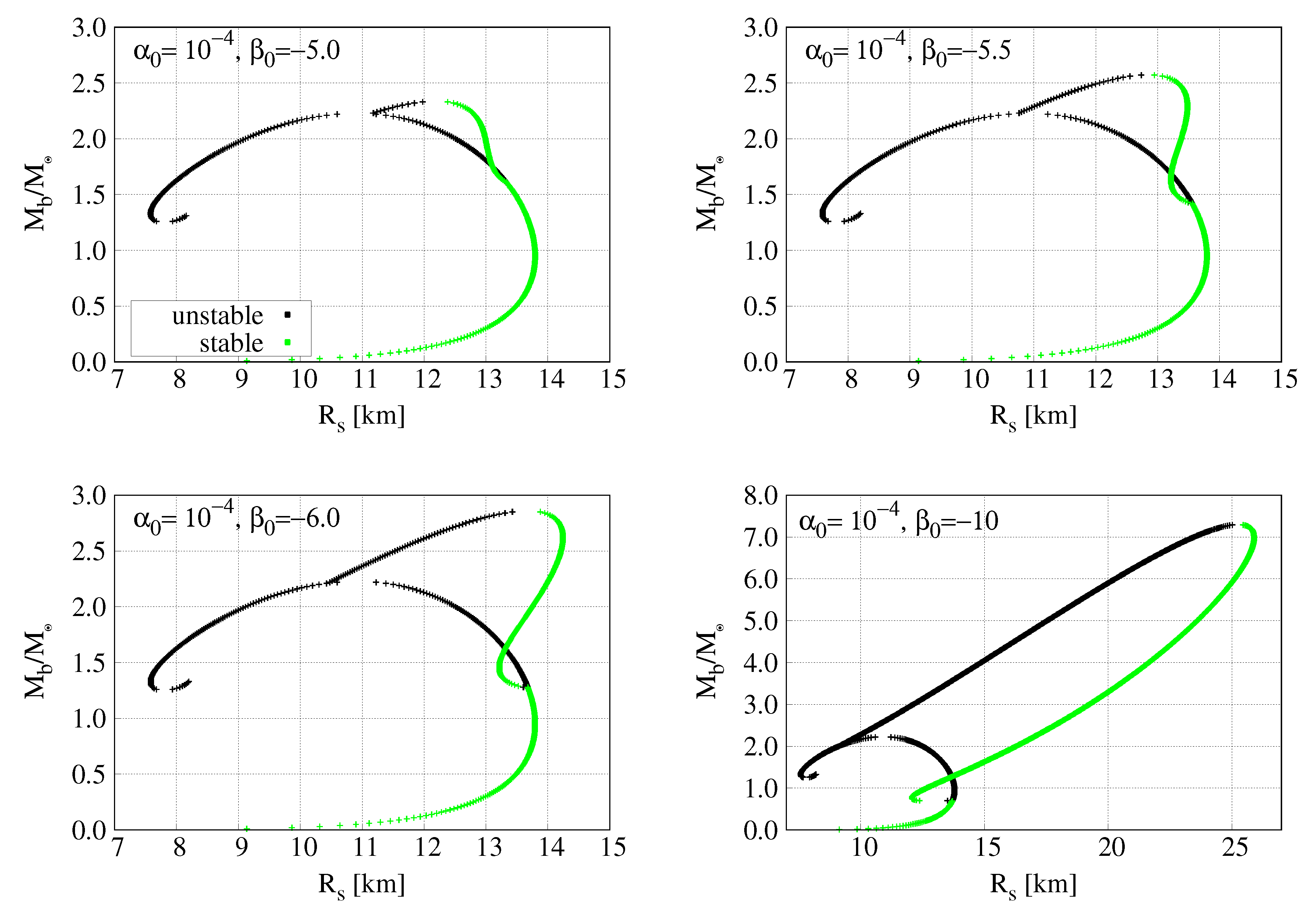
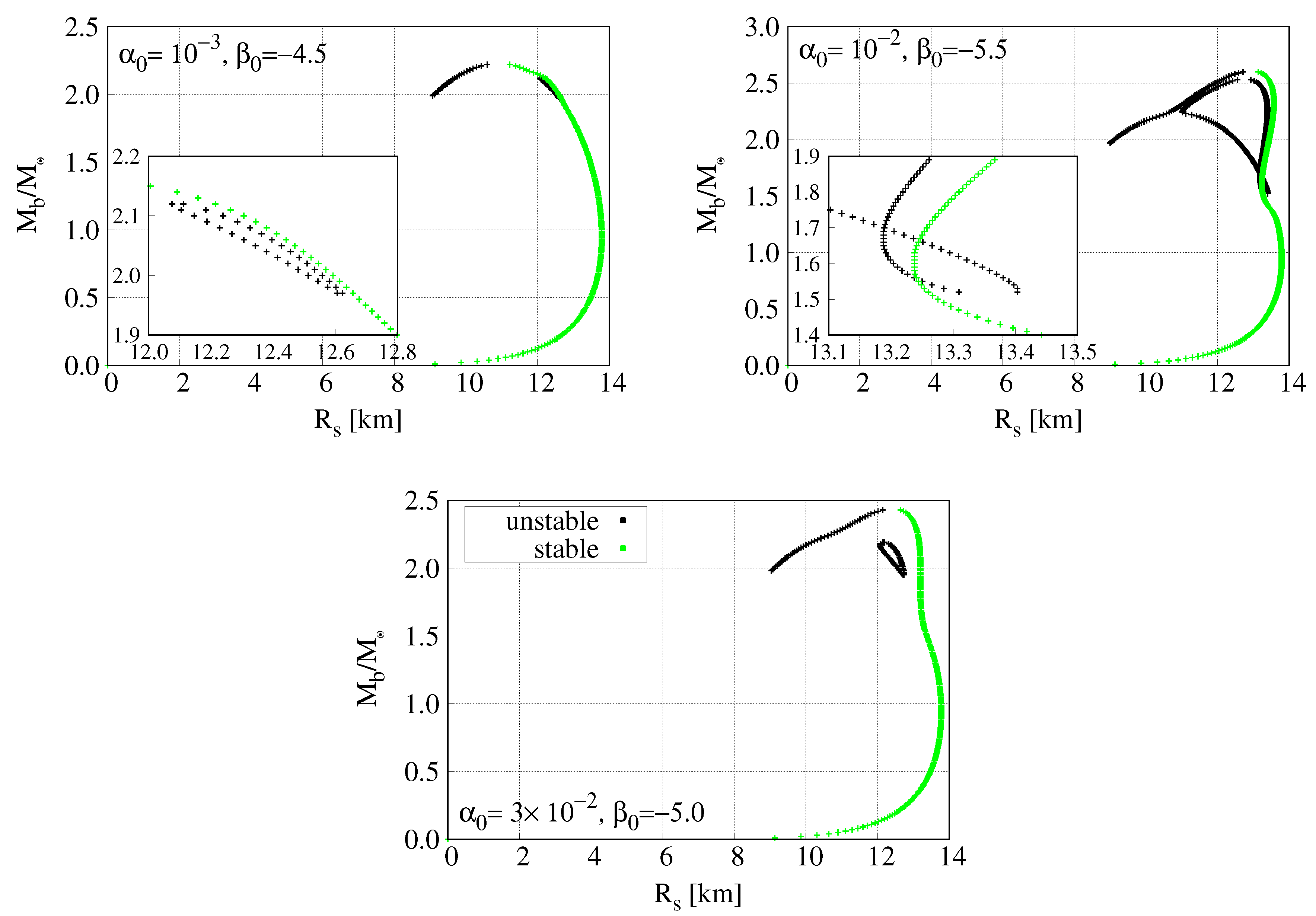
- Whenever multiple NS models with equal baryon mass exist, we find the scalarized model to be the stable configurations in the sense of minimal binding energy. Typically, though not always, this is the model with the largest radius; cf. Figure 8 and Figure 9. We also observe that the stable configurations agree in the sign of the central scalar field value, in our convention.
Author Contributions
Funding
Acknowledgments
Conflicts of Interest
References
- Will, C.M. The Confrontation between General Relativity and Experiment. Living Rev. Rel. 2014, 17, 4. [Google Scholar] [CrossRef] [PubMed]
- Abbott, B.P.; Abbott, R.; Abbott, T.D.; Abernathy, M.R.; Acernese, F.; Ackley, K.; Adams, C.; Adams, T.; Addesso, P.; Adhikari, R.X.; et al. Observation of Gravitational Waves from a Binary Black Hole Merger. Phys. Rev. Lett. 2016, 116, 061102. [Google Scholar] [CrossRef] [PubMed]
- Abbott, B.P.; Abbott, R.; Abbott, T.D.; Abernathy, M.R.; Acernese, F.; Ackley, K.; Adams, C.; Adams, T.; Addesso, P.; Adhikari, R.X.; et al. Tests of general relativity with GW150914. Phys. Rev. Lett. 2016, 116, 221101, Erratum in 2018, 121, 129902. [Google Scholar] [CrossRef] [PubMed]
- Abbott, B.P.; Abbott, R.; Abbott, T.D.; Acernese, F.; Ackley, K.; Adams, C.; Adams, T.; Addesso, P.; Adhikari, R.X.; Adya, V.B.; et al. Gravitational Waves and Gamma-rays from a Binary Neutron Star Merger: GW170817 and GRB 170817A. Astrophys. J. Lett. 2017, 848, L13. [Google Scholar] [CrossRef]
- Abbott, B.P.; Abbott, R.; Abbott, T.D.; Acernese, F.; Ackley, K.; Adams, C.; Adams, T.; Addesso, P.; Adhikari, R.X.; Adya, V.B.; et al. Tests of General Relativity with GW170817. Phys. Rev. Lett. 2019, 123, 011102. [Google Scholar] [CrossRef]
- Abbott, B.P.; Abbott, R.; Abbott, T.D.; Acernese, F.; Ackley, K.; Adams, C.; Adams, T.; Addesso, P.; Adhikari, R.X.; Adya, V.B.; et al. Tests of General Relativity with the Binary Black Hole Signals from the LIGO-Virgo Catalog GWTC-1. Phys. Rev. 2019, D100, 104036. [Google Scholar] [CrossRef]
- Yunes, N.; Yagi, K.; Pretorius, F. Theoretical Physics Implications of the Binary Black-Hole Mergers GW150914 and GW151226. Phys. Rev. 2016, D94, 084002. [Google Scholar] [CrossRef]
- Clifton, T.; Ferreira, P.G.; Padilla, A.; Skordis, C. Modified Gravity and Cosmology. Phys. Rept. 2012, 513, 1–189. [Google Scholar] [CrossRef]
- Berti, E.; Barausse, E.; Cardoso, V.; Gualtieri, L.; Pani, P.; Sperhake, U.; Stein, L.C.; Wex, N.; Yagi, K.; Baker, T.; et al. Testing General Relativity with Present and Future Astrophysical Observations. Class. Quant. Grav. 2015, 32, 243001. [Google Scholar] [CrossRef]
- Barack, L.; Cardoso, V.; Nissanke, S.; Sotiriou, T.P.; Askar, A.; Belczynski, C.; Bertone, G.; Bon, E.; Blas, D.; Brito, R.; et al. Black holes, gravitational waves and fundamental physics: A roadmap. Class. Quant. Grav. 2019, 36, 143001. [Google Scholar] [CrossRef]
- Olmo, G.J.; Rubiera-Garcia, D.; Wojnar, A. Stellar structure models in modified theories of gravity: Lessons and challenges. arXiv 2019, arXiv:gr-qc/1912.05202. [Google Scholar] [CrossRef]
- Capozziello, S.; D’Agostino, R.; Luongo, O. Extended Gravity Cosmography. Int. J. Mod. Phys. 2019, D28, 1930016. [Google Scholar] [CrossRef]
- Freese, K. Review of Observational Evidence for Dark Matter in the Universe and in upcoming searches for Dark Stars. EAS Publ. Ser. 2009, 36, 113–126. [Google Scholar] [CrossRef]
- Novosyadlyj, B.; Pelykh, V.; Shtanov, Y.; Zhuk, A. Dark Energy: Observational Evidence and Theoretical Models; Academperiodyka: Kyiv, Ukraine, 2013. [Google Scholar]
- Hamber, H.W. Quantum Gravitation: The Feynman Path Integral Approach; Springer: Berlin, Germany, 2009. [Google Scholar] [CrossRef]
- Lasky, P.D. Gravitational Waves from Neutron Stars: A Review. Publ. Astron. Soc. Austral. 2015, 32, e034. [Google Scholar] [CrossRef]
- Özel, F.; Freire, P. Masses, Radii, and the Equation of State of Neutron Stars. Ann. Rev. Astron. Astrophys. 2016, 54, 401–440. [Google Scholar] [CrossRef]
- Damour, T.; Esposito-Farese, G. Nonperturbative strong field effects in tensor–scalar theories of gravitation. Phys. Rev. Lett. 1993, 70, 2220–2223. [Google Scholar] [CrossRef]
- Damour, T.; Esposito-Farese, G. Tensor–scalar gravity and binary pulsar experiments. Phys. Rev. 1996, D54, 1474–1491. [Google Scholar] [CrossRef]
- Harada, T. Neutron stars in scalar tensor theories of gravity and catastrophe theory. Phys. Rev. 1998, D57, 4802–4811. [Google Scholar] [CrossRef]
- Ramazanoğlu, F.M.; Pretorius, F. Spontaneous Scalarization with Massive Fields. Phys. Rev. 2016, D93, 064005. [Google Scholar] [CrossRef]
- Bergmann, P.G. Comments on the scalar tensor theory. Int. J. Theor. Phys. 1968, 1, 25–36. [Google Scholar] [CrossRef]
- Wagoner, R.V. Scalar tensor theory and gravitational waves. Phys. Rev. 1970, D1, 3209–3216. [Google Scholar] [CrossRef]
- Andreou, N.; Franchini, N.; Ventagli, G.; Sotiriou, T.P. Spontaneous scalarization in generalised scalar-tensor theory. Phys. Rev. 2019, D99, 124022, Erratum in 2020, 101, 109903. [Google Scholar]
- Ventagli, G.; Lehébel, A.; Sotiriou, T.P. The onset of spontaneous scalarization in generalised scalar-tensor theories. arXiv 2020, arXiv:gr-qc/2006.01153. [Google Scholar]
- Silva, H.O.; Sakstein, J.; Gualtieri, L.; Sotiriou, T.P.; Berti, E. Spontaneous scalarization of black holes and compact stars from a Gauss-Bonnet coupling. Phys. Rev. Lett. 2018, 120, 131104. [Google Scholar] [CrossRef]
- Doneva, D.D.; Yazadjiev, S.S. New Gauss-Bonnet Black Holes with Curvature-Induced Scalarization in Extended Scalar-Tensor Theories. Phys. Rev. Lett. 2018, 120, 131103. [Google Scholar] [CrossRef]
- Barausse, E.; Jacobson, T.; Sotiriou, T.P. Black holes in Einstein-aether and Horava-Lifshitz gravity. Phys. Rev. 2011, D83, 124043. [Google Scholar] [CrossRef]
- Ramazanoğlu, F.M. Spontaneous growth of vector fields in gravity. Phys. Rev. 2017, D96, 064009. [Google Scholar] [CrossRef]
- Annulli, L.; Cardoso, V.; Gualtieri, L. Electromagnetism and hidden vector fields in modified gravity theories: Spontaneous and induced vectorization. Phys. Rev. 2019, D99, 044038. [Google Scholar] [CrossRef]
- Ramazanoğlu, F.M. Spontaneous tensorization from curvature coupling and beyond. Phys. Rev. 2019, D99, 084015. [Google Scholar] [CrossRef]
- Sotani, H. Slowly Rotating Relativistic Stars in Scalar-Tensor Gravity. Phys. Rev. 2012, D86, 124036. [Google Scholar] [CrossRef]
- Pani, P.; Berti, E. Slowly rotating neutron stars in scalar-tensor theories. Phys. Rev. 2014, D90, 024025. [Google Scholar] [CrossRef]
- Silva, H.O.; Macedo, C.F.B.; Berti, E.; Crispino, L.C.B. Slowly rotating anisotropic neutron stars in general relativity and scalar–tensor theory. Class. Quant. Grav. 2015, 32, 145008. [Google Scholar] [CrossRef]
- Yazadjiev, S.S.; Doneva, D.D.; Popchev, D. Slowly rotating neutron stars in scalar-tensor theories with a massive scalar field. Phys. Rev. 2016, D93, 084038. [Google Scholar] [CrossRef]
- Altaha Motahar, Z.; Blázquez-Salcedo, J.L.; Kleihaus, B.; Kunz, J. Scalarization of neutron stars with realistic equations of state. Phys. Rev. 2017, D96, 064046. [Google Scholar] [CrossRef]
- Staykov, K.V.; Popchev, D.; Doneva, D.D.; Yazadjiev, S.S. Static and slowly rotating neutron stars in scalar–tensor theory with self-interacting massive scalar field. Eur. Phys. J. 2018, C78, 586. [Google Scholar] [CrossRef] [PubMed]
- Doneva, D.D.; Yazadjiev, S.S.; Stergioulas, N.; Kokkotas, K.D. Rapidly rotating neutron stars in scalar-tensor theories of gravity. Phys. Rev. 2013, D88, 084060. [Google Scholar] [CrossRef]
- Doneva, D.D.; Yazadjiev, S.S.; Staykov, K.V.; Kokkotas, K.D. Universal I-Q relations for rapidly rotating neutron and strange stars in scalar-tensor theories. Phys. Rev. 2014, D90, 104021. [Google Scholar] [CrossRef]
- Doneva, D.D.; Yazadjiev, S.S.; Stergioulas, N.; Kokkotas, K.D. Differentially rotating neutron stars in scalar-tensor theories of gravity. Phys. Rev. 2018, D98, 104039. [Google Scholar] [CrossRef]
- Sotani, H.; Kokkotas, K.D. Maximum mass limit of neutron stars in scalar-tensor gravity. Phys. Rev. 2017, D95, 044032. [Google Scholar] [CrossRef]
- Rezaei, Z.; Dezdarani, H.Y. Ferromagnetic Neutron Stars in Scalar-Tensor Theories of Gravity. JCAP 2019, 1903, 013. [Google Scholar] [CrossRef]
- Anderson, D.; Yunes, N. Scalar charges and scaling relations in massless scalar–tensor theories. Class. Quant. Grav. 2019, 36, 165003. [Google Scholar] [CrossRef]
- Morisaki, S.; Suyama, T. Spontaneous scalarization with an extremely massive field and heavy neutron stars. Phys. Rev. 2017, D96, 084026. [Google Scholar] [CrossRef]
- Sotani, H.; Kokkotas, K.D. Compactness of neutron stars and Tolman VII solutions in scalar-tensor gravity. Phys. Rev. 2018, D97, 124034. [Google Scholar] [CrossRef]
- Tsuchida, T.; Kawamura, G.; Watanabe, K. A Maximum mass-to-size ratio in scalar tensor theories of gravity. Prog. Theor. Phys. 1998, 100, 291–313. [Google Scholar] [CrossRef]
- Abbott, R.; Abbott, T.D.; Abraham, S.; Acernese, F.; Ackley, K.; Adams, C.; Adhikari, R.X.; Adya, V.B.; Affeldt, C.; Agathos, M. GW190814: Gravitational Waves from the Coalescence of a 23 Solar Mass Black Hole with a 2.6 Solar Mass Compact Object. Astrophys. J. 2020, 896, L44. [Google Scholar] [CrossRef]
- Novak, J. Neutron star transition to strong scalar field state in tensor scalar gravity. Phys. Rev. 1998, D58, 064019. [Google Scholar] [CrossRef]
- Mendes, R.F.P.; Matsas, G.E.A.; Vanzella, D.A.T. Instability of nonminimally coupled scalar fields in the spacetime of slowly rotating compact objects. Phys. Rev. 2014, D90, 044053. [Google Scholar] [CrossRef]
- Mendes, R.F.P. Possibility of setting a new constraint to scalar-tensor theories. Phys. Rev. 2015, D91, 064024. [Google Scholar] [CrossRef]
- Mendes, R.F.P.; Ortiz, N. Highly compact neutron stars in scalar-tensor theories of gravity: Spontaneous scalarization versus gravitational collapse. Phys. Rev. 2016, D93, 124035. [Google Scholar] [CrossRef]
- Palenzuela, C.; Liebling, S.L. Constraining scalar-tensor theories of gravity from the most massive neutron stars. Phys. Rev. 2016, D93, 044009. [Google Scholar] [CrossRef]
- Bertotti, B.; Iess, L.; Tortora, P. A test of general relativity using radio links with the Cassini spacecraft. Nature 2003, 425, 374–376. [Google Scholar] [CrossRef] [PubMed]
- Williams, J.G.; Turyshev, S.G.; Boggs, D.H. Lunar laser ranging tests of the equivalence principle with the earth and moon. Int. J. Mod. Phys. 2009, D18, 1129–1175. [Google Scholar] [CrossRef]
- Wex, N. Testing Relativistic Gravity with Radio Pulsars. arXiv 2014, arXiv:gr-qc/1402.5594. [Google Scholar]
- Novak, J. Spherical neutron star collapse in tensor–scalar theory of gravity. Phys. Rev. 1998, D57, 4789–4801. [Google Scholar] [CrossRef]
- Novak, J.; Ibanez, J.M. Gravitational waves from the collapse and bounce of a stellar core in tensor scalar gravity. Astrophys. J. 2000, 533, 392–405. [Google Scholar] [CrossRef]
- Gerosa, D.; Sperhake, U.; Ott, C.D. Numerical simulations of stellar collapse in scalar-tensor theories of gravity. Class. Quant. Grav. 2016, 33, 135002. [Google Scholar] [CrossRef]
- Barausse, E.; Palenzuela, C.; Ponce, M.; Lehner, L. Neutron-star mergers in scalar-tensor theories of gravity. Phys. Rev. 2013, D87, 081506. [Google Scholar] [CrossRef]
- Palenzuela, C.; Barausse, E.; Ponce, M.; Lehner, L. Dynamical scalarization of neutron stars in scalar-tensor gravity theories. Phys. Rev. 2014, D89, 044024. [Google Scholar] [CrossRef]
- Shibata, M.; Taniguchi, K.; Okawa, H.; Buonanno, A. Coalescence of binary neutron stars in a scalar-tensor theory of gravity. Phys. Rev. 2014, D89, 084005. [Google Scholar] [CrossRef]
- Chen, P.; Suyama, T.; Yokoyama, J. Spontaneous scalarization: Asymmetron as dark matter. Phys. Rev. 2015, D92, 124016. [Google Scholar] [CrossRef]
- Doneva, D.D.; Yazadjiev, S.S. Rapidly rotating neutron stars with a massive scalar field—structure and universal relations. JCAP 2016, 1611, 019. [Google Scholar] [CrossRef]
- Sperhake, U.; Moore, C.J.; Rosca, R.; Agathos, M.; Gerosa, D.; Ott, C.D. Long-lived inverse chirp signals from core collapse in massive scalar-tensor gravity. Phys. Rev. Lett. 2017, 119, 201103. [Google Scholar] [CrossRef] [PubMed]
- Rosca-Mead, R.; Sperhake, U.; Moore, C.J.; Agathos, M.; Gerosa, D.; Ott, C.D. Core collapse in massive scalar-tensor gravity. arXiv 2020, arXiv:gr-qc/2005.09728. [Google Scholar] [CrossRef]
- Geng, C.Q.; Kuan, H.J.; Luo, L.W. Inverse-Chirp Imprint of Gravitational Wave Signals in Scalar Tensor Theory. arXiv 2020, arXiv:gr-qc/2005.11629. [Google Scholar]
- Cheong, P.C.K.; Li, T.G.F. Numerical studies on core collapse supernova in self-interacting massive scalar-tensor gravity. Phys. Rev. 2019, D100, 024027. [Google Scholar] [CrossRef]
- Rosca-Mead, R.; Moore, C.J.; Agathos, M.; Sperhake, U. Inverse-chirp signals and spontaneous scalarisation with self-interacting potentials in stellar collapse. Class. Quant. Grav. 2019, 36, 134003. [Google Scholar] [CrossRef]
- Fujii, Y.; Maeda, K. The Scalar-Tensor Theory of Gravitation; Cambridge Monographs on Mathematical Physics; Cambridge University Press: Cambridge, UK, 2007. [Google Scholar] [CrossRef]
- Salgado, M. The Cauchy problem of scalar tensor theories of gravity. Class. Quant. Grav. 2006, 23, 4719–4742. [Google Scholar] [CrossRef]
- Faraoni, V.; Gunzig, E. Einstein frame or Jordan frame? Int. J. Theor. Phys. 1999, 38, 217–225. [Google Scholar] [CrossRef]
- Salgado, M.; Martinez-del Rio, D.; Alcubierre, M.; Nunez, D. Hyperbolicity of scalar-tensor theories of gravity. Phys. Rev. 2008, D77, 104010. [Google Scholar] [CrossRef]
- Geng, C.Q.; Kuan, H.J.; Luo, L.W. Viable Constraint on Scalar Field in Scalar-Tensor Theory. Class. Quant. Grav. 2020, 37, 115001. [Google Scholar] [CrossRef]
- Press, W.H.; Teukolsky, S.A.; Flannery, B.P.; Vetterling, W.T. Numerical Recipes in C (2nd ed.): The Art of Scientific Computing; Cambridge University Press: New York, NY, USA, 1992. [Google Scholar]
- Shapiro, S.L.; Teukolsky, S.A. Black Holes, White Dwarfs, and Neutron Stars; John Wiley & Sons, Inc.: Hoboken, NJ, USA, 1983. [Google Scholar]
- Arnowitt, R.L.; Deser, S.; Misner, C.W. The Dynamics of general relativity. Gen. Rel. Grav. 2008, 40, 1997–2027. [Google Scholar] [CrossRef]
- Brito, R.; Cardoso, V.; Macedo, C.F.B.; Okawa, H.; Palenzuela, C. Interaction between bosonic dark matter and stars. Phys. Rev. 2016, D93, 044045. [Google Scholar] [CrossRef]
- Baumann, D.; Chia, H.S.; Stout, J.; ter Haar, L. The Spectra of Gravitational Atoms. JCAP 2019, 1912, 006. [Google Scholar] [CrossRef]
- Akmal, A.; Pandharipande, V.; Ravenhall, D. The Equation of state of nucleon matter and neutron star structure. Phys. Rev. 1998, C58, 1804–1828. [Google Scholar] [CrossRef]
- Read, J.S.; Markakis, C.; Shibata, M.; Uryu, K.; Creighton, J.D.; Friedman, J.L. Measuring the neutron star equation of state with gravitational wave observations. Phys. Rev. 2009, D79, 124033. [Google Scholar] [CrossRef]


© 2020 by the authors. Licensee MDPI, Basel, Switzerland. This article is an open access article distributed under the terms and conditions of the Creative Commons Attribution (CC BY) license (http://creativecommons.org/licenses/by/4.0/).
Share and Cite
Rosca-Mead, R.; Moore, C.J.; Sperhake, U.; Agathos, M.; Gerosa, D. Structure of Neutron Stars in Massive Scalar-Tensor Gravity. Symmetry 2020, 12, 1384. https://doi.org/10.3390/sym12091384
Rosca-Mead R, Moore CJ, Sperhake U, Agathos M, Gerosa D. Structure of Neutron Stars in Massive Scalar-Tensor Gravity. Symmetry. 2020; 12(9):1384. https://doi.org/10.3390/sym12091384
Chicago/Turabian StyleRosca-Mead, Roxana, Christopher J. Moore, Ulrich Sperhake, Michalis Agathos, and Davide Gerosa. 2020. "Structure of Neutron Stars in Massive Scalar-Tensor Gravity" Symmetry 12, no. 9: 1384. https://doi.org/10.3390/sym12091384
APA StyleRosca-Mead, R., Moore, C. J., Sperhake, U., Agathos, M., & Gerosa, D. (2020). Structure of Neutron Stars in Massive Scalar-Tensor Gravity. Symmetry, 12(9), 1384. https://doi.org/10.3390/sym12091384