Convergence Analysis of Self-Adaptive Inertial Extra-Gradient Method for Solving a Family of Pseudomonotone Equilibrium Problems with Application

Abstract

In this article, we propose a new modified extragradient-like method to solve pseudomonotone equilibrium problems in real Hilbert space with a Lipschitz-type condition on a bifunction. This method uses a variable stepsize formula that is updated at each iteration based on the previous iterations. The advantage of the method is that it operates without prior knowledge of Lipschitz-type constants and any line search method. The weak convergence of the method is established by taking mild conditions on a bifunction. In the context of an application, fixed-point theorems involving strict pseudo-contraction and results for pseudomonotone variational inequalities are considered. Many numerical results have been reported to explain the numerical behavior of the proposed method.

1. Introduction

Let $\mathcal{C}$ be a nonempty, closed and convex subset of a real Hilbert space $\mathcal{H}$ and $\mathcal{R},$ $\mathcal{N}$ be the sets of real numbers and natural numbers, respectively. Assume that f is a bifunction $f:\mathcal{H}\times \mathcal{H}\to \mathcal{R}$ and $EP(f,\mathcal{C})$ denotes the solution set of an equilibrium problem over the set $\mathcal{C}.$ Now, consider the following definitions of a bifunction monotonicity (see [1,2] for more details). A function $f:\mathcal{H}\times \mathcal{H}\to \mathcal{R}$ on $\mathcal{C}$ for $\gamma >0$ is said to be:

(1)

γ-strongly monotone if

$$f(z_1,z_2)+f(z_2,z_1)\le -\gamma {\parallel z_1-z_2\parallel }^2,\forall z_1,z_2\in \mathcal{C};$$

(2)

monotone if

$$f(z_1,z_2)+f(z_2,z_1)\le 0,\forall z_1,z_2\in \mathcal{C};$$

(3)

γ-strongly pseudomonotone if

$$f(z_1,z_2)\ge 0⟹f(z_2,z_1)\le -\gamma {\parallel z_1-z_2\parallel }^2,\forall z_1,z_2\in \mathcal{C};$$

(4)

pseudomonotone if

$$f(z_1,z_2)\ge 0⟹f(z_2,z_1)\le 0,\forall z_1,z_2\in \mathcal{C}.$$

It is clear from the definitions mentioned above that they have the following consequences:

$$\left(1\right)⟹\left(2\right)⟹\left(4\right)\mathrm{and}\left(1\right)⟹\left(3\right)⟹\left(4\right).$$

In general, the converses are not true. A bifunction $f:\mathcal{H}\times \mathcal{H}\to \mathcal{R}$ is said to be Lipschitz-type continuous on $\mathcal{C}$ if there exist two positive constants $c_1,c_2$ such that

$$f(z_1,z_3)\le f(z_1,z_2)+f(z_2,z_3)+c_1\parallel z_1-z_2{\parallel }^2+c_2{\parallel z_2-z_3\parallel }^2,\forall z_1,z_2,z_3\in \mathcal{C}.$$

Let $\mathcal{C}$ be a nonempty closed convex subset of $\mathcal{H}$ and $f:\mathcal{H}\times \mathcal{H}\to \mathcal{R}$ be a bifunction with $f(z_1,z_1)=0,$ for all $z_1\in \mathcal{C}.$ An equilibrium problem [1,3] for f on the set $\mathcal{C}$ is to

$$\mathrm{find}{u}^{*}\in \mathcal{C}\mathrm{such}\mathrm{that}f(u^{*},z_1)\ge 0,\forall z_1\in \mathcal{C}.$$

(1)

An equilibrium problem (1) had many mathematical problems as a particular case, i.e., the variational inequality problems (VIP), optimization problems, fixed point problems, complementarity problems, the Nash equilibrium of non-cooperative games, saddle point problems and the vector optimization problem (for details see [1,4,5]). The equilibrium problem is also known as the famous Ky Fan inequality [3]. However, the particular format of an equilibrium problem (1) was initiated by Muu and Oettli [6] in 1992 and further investigation on its theoretical properties were provided by Blum and Oettli [1]. The construction of new iterative schemes and the modification of existing methods, as well as the study their convergence analysis, constitute an important research direction in equilibrium problem theory. Several methods have been developed in the past few years to approximate the solution of an equilibrium problem in finite and infinite dimensional real Hilbert spaces, i.e., extragradient methods [7,8,9,10,11,12,13,14,15,16], subgradient methods [17,18,19,20,21,22], inertial methods [23,24,25] and methods for particular classes of equilibrium problems [26,27,28,29,30,31,32,33,34,35].

In particular, a proximal method [36] was used to solve equilibrium problems based on solving minimization problems. This approach was also known as the two-step extragradient-like method in [7] due to the early contribution of the Korpelevich [37] extragradient method to solve the saddle point problems. More precisely, Tran et al. introduced a method in [7], and an iterative sequence $\{u_n\}$ was generated as follows:

$$\left\{\begin{array}{c}{u}_0\in \mathcal{C},\hfill \\ v_n=\underset{}{argmin}\{\lambda f(u_n,v)+\frac{1}{2}\parallel u_n-v{\parallel }^2:v\in \mathcal{C}\},\hfill \\ u_{n+1}=\underset{}{argmin}\{\lambda f(v_n,v)+\frac{1}{2}\parallel u_n-v{\parallel }^2:v\in \mathcal{C}\},\hfill \end{array}\right.$$

where $0<\lambda <min\left\{\frac{1}{2c_1},\frac{1}{2c_2}\right\}$. The iterative sequence generated from the above-mentioned method provides a weak convergent iterative sequence and in order to operate it, prior information regarding the Lipschitz-type constants is required. These Lipschitz-type constants are mostly unknown or hard to compute. To overcome this situation, Hieu et al. [14] introduced an extension of the method in [38] for solving the equilibrium problem as follows: Let ${\left[t\right]}_{+}:=max\{t,0\}$ and choose $u_0\in \mathcal{C},$ $\mu \in (0,1)$ with ${\lambda }_0>0$ such that

$$\left\{\begin{array}{c}{v}_n=\underset{}{argmin}\{{\lambda }_{n}f(u_n,v)+\frac{1}{2}\parallel u_n-v{\parallel }^2:v\in \mathcal{C}\},\hfill \\ u_{n+1}=\underset{}{argmin}\{{\lambda }_{n}f(v_n,v)+\frac{1}{2}\parallel u_n-v{\parallel }^2:v\in \mathcal{C}\},\hfill \end{array}\right.$$

where the stepsize sequence $\{{\lambda }_n\}$ is updated in the following way:

$${\lambda }_{n+1}=min\left\{{\lambda }_n,\frac{\mu (\parallel u_n-v_n{\parallel }^2+\parallel u_{n+1}-v_n{\parallel }^2)}{2{[f(u_n,u_{n+1})-f(u_n,v_n)-f(v_n,u_{n+1})]}_{+}}\right\}.$$

Recently, Vinh and Muu proposed an inertial iterative algorithm in [39] to solve a pseudomonotone equilibrium problem. Their main contribution is the availability of an inertial effect in the algorithm that is used to improve the convergence rate of the iterative sequence. The iterative sequence $\{u_n\}$ has been generated in the following manner:

(i)

Choose $u_{-1},u_0\in \mathcal{C},$ $\vartheta \in [0,1),$ $0<\lambda <min\{\frac{1}{2c_1},\frac{1}{2c_2}\}$ while a sequence $\{{ϵ}_n\}\subset [0,+\infty )$ is satisfying the following condition:

$$\sum _{n=0}^{+\infty }{ϵ}_n<+\infty .$$

(2)

(ii)

Choose ${\vartheta }_n$ such that $0\le {\vartheta }_n\le \overline{{\vartheta }_n}$ where

$$\overline{{\vartheta }_n}=\left\{\begin{array}{cc}min\left\{\vartheta ,\frac{{ϵ}_n}{\parallel u_n-u_{n-1}\parallel }\right\}\hfill & \mathrm{if}{u}_n\ne u_{n-1},\hfill \\ \vartheta \hfill & \mathrm{otherwise}.\hfill \end{array}\right.$$

(3)

(iii)

Determine

$$\left\{\begin{array}{c}{\eta }_n=u_n+{\vartheta }_n(u_n-u_{n-1}),\hfill \\ v_n=\underset{}{argmin}\{\lambda f({\eta }_n,v)+\frac{1}{2}\parallel {\eta }_n-v{\parallel }^2:v\in \mathcal{C}\},\hfill \\ u_{n+1}=\underset{}{argmin}\{\lambda f(v_n,v)+\frac{1}{2}\parallel {\eta }_n-v{\parallel }^2:v\in \mathcal{C}\}.\hfill \end{array}\right.$$

This article focuses on projection methods that are well-known and easy to execute due to their efficient and straightforward mathematical computation. Motivated by the works of [14,40], we formulate an inertial explicit subgradient extragradient algorithm to solve the pseudomonotone equilibrium problem. The proposed algorithm can be seen as the modification of the methods that appear in [7,14,39]. Under certain mild conditions, a weak convergence result has been proven to correspond to the iterative sequence of the algorithm. Moreover, experimental studies have shown that the proposed method tends to be more efficient compared to the existing method [39].

The remainder of this paper is arranged as follows: Section 2 contains some definitions and basic results used in the paper. Section 3 contains our main algorithm and proves its convergence. Section 4 and Section 5 incorporate the implementation of our results. Section 6 carries out the numerical results that demonstrates the computational effectiveness of our proposed algorithm.

2. Background

   Let $h:\mathcal{C}\to \mathcal{R}$ be a convex function on a nonempty, closed and convex subset $\mathcal{C}$ of a real Hilbert space $\mathcal{H}$, and the subdifferential of a function h at $z_1\in \mathcal{C}$ is defined as:

$$\partial h\left(z_1\right)=\{z_3\in \mathcal{H}:h\left(z_2\right)-h\left(z_1\right)\ge ⟨z_3,z_2-z_1⟩,\forall z_2\in \mathcal{C}\}.$$

Let $\mathcal{C}$ be a nonempty, closed and convex subset of a real Hilbert space $\mathcal{H}$ and a normal cone of $\mathcal{C}$ at $z_1\in \mathcal{C}$ is defined by:

$$N_{\mathcal{C}}\left(z_1\right)=\{z_3\in \mathcal{H}:⟨z_3,z_2-z_1⟩\le 0,\forall z_2\in \mathcal{C}\}.$$

The metric projection $P_{\mathcal{C}}\left(z_1\right)$ for $z_1\in \mathcal{H}$ onto a closed and convex subset $\mathcal{C}$ of $\mathcal{H}$ is defined by:

$$P_{\mathcal{C}}\left(z_1\right)=\underset{}{argmin}\{\parallel z_2-z_1\parallel :z_2\in \mathcal{C}\}.$$

Lemma 1

([41]). Let $\mathcal{C}$ be a nonempty, closed and convex subset of a real Hilbert space $\mathcal{H}$ and $P_{\mathcal{C}}:\mathcal{H}\to \mathcal{C}$ be a metric projection from $\mathcal{H}$ onto $\mathcal{C}$.

(i)

Let $z_1\in \mathcal{C}$ and $z_2\in \mathcal{H};$ we have

$$\parallel z_1-P_{\mathcal{C}}\left(z_2\right){\parallel }^2+\parallel P_{\mathcal{C}}\left(z_2\right)-z_2{\parallel }^2\le {\parallel z_1-z_2\parallel }^2.$$

(ii)

$z_3=P_{\mathcal{C}}\left(z_1\right)$ if and only if

$$⟨z_1-z_3,z_2-z_3⟩\le 0,\forall z_2\in \mathcal{C}.$$

(iii)

For $z_2\in \mathcal{C}$ and $z_1\in \mathcal{H}$

$$\parallel z_1-P_{\mathcal{C}}\left(z_1\right)\parallel \le \parallel z_1-z_2\parallel .$$

Lemma 2

([42]). Let $h:\mathcal{C}\to \mathcal{R}$ be a convex, subdifferentiable and lower semicontinuous function on $\mathcal{C},$ where $\mathcal{C}$ is a nonempty, convex and closed subset of a real Hilbert space $\mathcal{H}.$ Then, an element $z_1\in \mathcal{C}$ is a minimizer of a function h if and only if $0\in \partial h\left(z_1\right)+N_{\mathcal{C}}\left(z_1\right),$ where $\partial h\left(z_1\right)$ and $N_{\mathcal{C}}\left(z_1\right)$ represent the subdifferential of h at $z_1\in \mathcal{C}$ and normal cone of $\mathcal{C}$ at $z_1$, respectively.

Lemma 3

([43]). Let $\{u_n\}$ be a sequence in $\mathcal{H}$ and $\mathcal{C}\subset \mathcal{H}$ such that the following conditions hold:

(i)

For each $u\in \mathcal{C},$ the ${lim}_{n\to \infty }\parallel u_n-u\parallel$ exists;

(ii)

Each sequentially weak cluster limit point of the sequence $\{u_n\}$ belongs to $\mathcal{C}$.

Then, the sequence $\{u_n\}$ weakly converges to some element in $\mathcal{C}.$

Lemma 4.

[44] Let $\{q_n\}$ and $\{p_n\}$ be sequences of non-negative real numbers satisfying $q_{n+1}\le q_n+p_n,$ for each $n\in \mathcal{N}.$ If $\sum p_n<\infty ,$ then ${lim}_{n\to \infty }{q}_n$ exists.

Assume that a bifunction f satisfies the following conditions:

(f1)

$f(z_2,z_2)=0,$ for all $z_2\in \mathcal{C}$ and f is pseudomonotone on $\mathcal{C};$

(f2)

f satisfies the Lipschitz-type condition on $\mathcal{H}$ through $c_1>0$ and $c_2>0;$

(f3)

$\underset{n\to \infty }{lim\; sup}f(z_n,v)\le f(z^{*},v)$ for every $v\in \mathcal{C}$ and $\{z_n\}\subset \mathcal{C}$ satisfying $z_n\rightharpoonup z^{*}$;

(f4)

$f(z_1,.)$ needs to be convex and subdifferentiable on $\mathcal{H}$ for each $z_1\in \mathcal{H}.$

3. Convergence Analysis for an Algorithm

We provide a method consisting of two strongly convex minimization problems through an inertial factor and an explicit stepsize formula, which are being used to improve the convergence rate of the iterative sequence and to make the method independent of the Lipschitz constants. The detailed method is provided below Algorithm 1:

Algorithm 1 (Inertial methods for pseudomonotone equilibrium problems)

Initialization: Choose $u_{-1},u_0\in \mathcal{C},$ $\mu \in (0,1),$ ${\lambda }_0>0,$ $\vartheta \in [0,1)$ and a sequence $\{{ϵ}_n\}\subset [0,+\infty )$ satisfying $$\sum _{n=0}^{+\infty }{ϵ}_n<+\infty .$$ (4) Iterative steps: Choose ${\vartheta }_n$ satisfying $0\le {\vartheta }_n\le \overline{{\vartheta }_n}$ and $$\overline{{\vartheta }_n}=\left\{\begin{array}{cc}min\left\{\vartheta ,\frac{{ϵ}_n}{\parallel u_n-u_{n-1}\parallel }\right\}\hfill & \mathrm{if}{u}_n\ne u_{n-1},\hfill \\ \vartheta \hfill & \mathrm{otherwise}.\hfill \end{array}\right.$$ (5) Step 1: Determine $$v_n=\underset{y\in \mathcal{C}}{argmin}\{{\lambda }_{n}f({\eta }_n,y)+\frac{1}{2}\parallel {\eta }_n-y{\parallel }^2\},$$ where ${\eta }_n=u_n+{\vartheta }_n(u_n-u_{n-1}).$ If ${\eta }_n=v_n$; STOP. Otherwise, go to next step. Step 2: Determine a half-space $${\mathcal{H}}_n=\{z\in \mathcal{H}:⟨{\eta }_n-{\lambda }_n{\omega }_n-v_n,z-v_n⟩\le 0\},$$ where ${\omega }_n\in {\partial }_{2}f({\eta }_n,v_n)$ and evaluate $$u_{n+1}=\underset{y\in {\mathcal{H}}_n}{argmin}\{{\lambda }_{n}f(v_n,y)+\frac{1}{2}\parallel {\eta }_n-y{\parallel }^2\}.$$ Step 3: Set $d_1=f({\eta }_n,u_{n+1})-f({\eta }_n,v_n)-f(v_n,u_{n+1})$ and evaluate $${\lambda }_{n+1}=\left\{\begin{array}{cc}min\left\{{\lambda }_n,\frac{\mu \parallel {\eta }_n-v_n{\parallel }^2+\mu {\parallel u_{n+1}-v_n\parallel }^2}{2d_1}\right\}\mathrm{if}\hfill & d_1>0,\hfill \\ {\lambda }_n\hfill & \mathrm{otherwise}.\end{array}\right.$$ Set $n:=n+1$ and go back to Iterative steps.

Lemma 5.

The sequence $\{{\lambda }_n\}$ is decreasing monotonically with a lower bound $min\left\{\frac{\mu }{2max\{c_1,c_2\}},{\lambda }_0\right\}$ and converges to $\lambda >0.$

Proof. 

From the definition of $\{{\lambda }_n\},$ we see that this sequence is monotone and non-increasing. It is given that f satisfies the Lipschitz-type condition with constants $c_1$ and $c_2$. Let $f({\eta }_n,u_{n+1})-f({\eta }_n,v_n)-f(v_n,u_{n+1})>0,$ such that

$$\begin{array}{cc}\hfill \frac{\mu (\parallel {\eta }_n-v_n{\parallel }^2+\parallel u_{n+1}-v_n{\parallel }^2)}{2[f({\eta }_n,u_{n+1})-f({\eta }_n,v_n)-f(v_n,u_{n+1})]}& \ge \frac{\mu (\parallel {\eta }_n-v_n{\parallel }^2+\parallel u_{n+1}-v_n{\parallel }^2)}{2[c_1\parallel {\eta }_n-v_n{\parallel }^2+c_2\parallel u_{n+1}-v_n{\parallel }^2]}\hfill \\ \hfill & \ge \frac{\mu }{2max\{c_1,c_2\}}.\hfill \end{array}$$

(6)

The above implies that the sequence $\{{\lambda }_n\}$ has a lower bound $min\left\{\frac{\mu }{2max\{c_1,c_2\}},{\lambda }_0\right\}.$ Moreover, there exists a real number $\lambda >0,$ such that ${lim}_{n\to \infty }{\lambda }_n=\lambda .$ □

Remark 1.

Due to the summability of ${\displaystyle \sum _{n=0}^{+\infty }{ϵ}_n}$, Expression (5) implies that:

$$\sum _{n=1}^{\infty }{\vartheta }_n\parallel u_n-u_{n-1}\parallel \le \sum _{n=1}^{\infty }\overline{{\vartheta }_n}\parallel u_n-u_{n-1}\parallel \le \sum _{n=1}^{\infty }\vartheta \parallel u_n-u_{n-1}\parallel <\infty ,$$

(7)

which implies that:

$$\underset{n\to \infty }{lim}\vartheta \parallel u_n-u_{n-1}\parallel =0.$$

(8)

Lemma 6.

Assume that a bifunction $f:\mathcal{H}\times \mathcal{H}\to \mathcal{R}$ satisfies the conditions (f1)–(f4). For each $u^{*}\in EP(f,\mathcal{C})\ne \varnothing ,$ we have

$$\parallel u_{n+1}-u^{*}{\parallel }^2\le \parallel {\eta }_n-u^{*}{\parallel }^2-\left(1-\frac{\mu {\lambda }_n}{{\lambda }_{n+1}}\right)\parallel {\eta }_n-v_n{\parallel }^2-\left(1-\frac{\mu {\lambda }_n}{{\lambda }_{n+1}}\right){\parallel u_{n+1}-v_n\parallel }^2.$$

Proof. 

From the value of $u_{n+1},$ we have

$$0\in {\partial }_2\left\{{\lambda }_{n}f(v_n,y)+\frac{1}{2}{\parallel {\eta }_n-y\parallel }^2\right\}\left(u_{n+1}\right)+N_{{\mathcal{H}}_n}\left(u_{n+1}\right).$$

For some $\omega \in \partial f(v_n,u_{n+1})$ there exists $\overline{\omega }\in N_{{\mathcal{H}}_n}\left(u_{n+1}\right)$ such that

$${\lambda }_n\omega +u_{n+1}-{\eta }_n+\overline{\omega }=0.$$

The above equality implies that

$$⟨{\eta }_n-u_{n+1},y-u_{n+1}⟩={\lambda }_n⟨\omega ,y-u_{n+1}⟩+⟨\overline{\omega },y-u_{n+1}⟩,\forall y\in {\mathcal{H}}_n.$$

Since $\overline{\omega }\in N_{{\mathcal{H}}_n}\left(u_{n+1}\right),$ it follows that $⟨\overline{\omega },y-u_{n+1}⟩\le 0,$ for all $y\in {\mathcal{H}}_n.$ Thus, we have

$$⟨{\eta }_n-u_{n+1},y-u_{n+1}⟩\le {\lambda }_n⟨\omega ,y-u_{n+1}⟩,\forall y\in {\mathcal{H}}_n.$$

(9)

Further, $\omega \in \partial f(v_n,u_{n+1})$ and due to the definition of subdifferential, we have

$$f(v_n,y)-f(v_n,u_{n+1})\ge ⟨\omega ,y-u_{n+1}⟩,\forall y\in \mathcal{H}.$$

(10)

Combining Expressions (9) and (10), we obtain

$${\lambda }_{n}f(v_n,y)-{\lambda }_{n}f(v_n,u_{n+1})\ge ⟨{\eta }_n-u_{n+1},y-u_{n+1}⟩,\forall y\in {\mathcal{H}}_n.$$

(11)

From the definition of ${\mathcal{H}}_n,$ we can write

$${\lambda }_n⟨{\omega }_n,u_{n+1}-v_n⟩\ge ⟨{\eta }_n-v_n,u_{n+1}-v_n⟩.$$

(12)

Due to ${\omega }_n\in \partial f({\eta }_n,v_n)$, we have

$$f({\eta }_n,y)-f({\eta }_n,v_n)\ge ⟨{\omega }_n,y-v_n⟩,\forall y\in \mathcal{H}.$$

By substituting $y=u_{n+1}$ in the above expression, we have

$$f({\eta }_n,u_{n+1})-f({\eta }_n,v_n)\ge ⟨{\omega }_n,u_{n+1}-v_n⟩,\forall y\in \mathcal{H}.$$

(13)

Combining Expressions (12) and (13), we obtain

$${\lambda }_n\left\{f({\eta }_n,u_{n+1})-f({\eta }_n,v_n)\right\}\ge ⟨{\eta }_n-v_n,u_{n+1}-v_n⟩.$$

(14)

By substituting $y=u^{*}$ in Expression (11), we have

$${\lambda }_{n}f(v_n,u^{*})-{\lambda }_{n}f(v_n,u_{n+1})\ge ⟨{\eta }_n-u_{n+1},u^{*}-u_{n+1}⟩.$$

(15)

Since $u^{*}\in EP(f,\mathcal{C})$, we have $f(u^{*},v_n)\ge 0.$ From the pseudomonotonicity of bifunction f, we obtain $f(v_n,u^{*})\le 0.$ Hence, it follows from Expression (15) that

$$⟨{\eta }_n-u_{n+1},u_{n+1}-u^{*}⟩\ge {\lambda }_{n}f(v_n,u_{n+1}).$$

(16)

From the definition of ${\lambda }_{n+1},$ we obtain

$$f({\eta }_n,u_{n+1})-f({\eta }_n,v_n)-f(v_n,u_{n+1})\le \frac{\mu \parallel {\eta }_n-v_n{\parallel }^2+\mu {\parallel u_{n+1}-v_n\parallel }^2}{2{\lambda }_{n+1}}$$

(17)

From Expressions (16) and (17), we have

$$\begin{array}{cc}\hfill ⟨{\eta }_n-u_{n+1},u_{n+1}-u^{*}⟩& \ge {\lambda }_n\{f({\eta }_n,u_{n+1})-f({\eta }_n,v_n)\}\hfill \\ \hfill & -\frac{\mu {\lambda }_n}{2{\lambda }_{n+1}}\parallel {\eta }_n-v_n{\parallel }^2-\frac{\mu {\lambda }_n}{2{\lambda }_{n+1}}{\parallel u_{n+1}-v_n\parallel }^2.\hfill \end{array}$$

(18)

Combining Expressions (14) and (18), we obtain

$$\begin{array}{cc}\hfill ⟨{\eta }_n-u_{n+1},u_{n+1}-u^{*}⟩& \ge ⟨{\eta }_n-v_n,u_{n+1}-v_n⟩\hfill \\ \hfill & -\frac{\mu {\lambda }_n}{2{\lambda }_{n+1}}\parallel {\eta }_n-v_n{\parallel }^2-\frac{\mu {\lambda }_n}{2{\lambda }_{n+1}}{\parallel u_{n+1}-v_n\parallel }^2.\hfill \end{array}$$

(19)

We have the following formulas:

$$-2⟨{\eta }_n-u_{n+1},u_{n+1}-u^{*}⟩=-\parallel {\eta }_n-u^{*}{\parallel }^2+\parallel u_{n+1}-{\eta }_n{\parallel }^2+{\parallel u_{n+1}-u^{*}\parallel }^2.$$

(20)

$$2⟨v_n-{\eta }_n,v_n-u_{n+1}⟩=\parallel {\eta }_n-v_n{\parallel }^2+\parallel u_{n+1}-v_n{\parallel }^2-{\parallel {\eta }_n-u_{n+1}\parallel }^2.$$

(21)

Combining the relations (19)–(21), we get

$$\parallel u_{n+1}-u^{*}{\parallel }^2\le \parallel {\eta }_n-u^{*}{\parallel }^2-\left(1-\frac{\mu {\lambda }_n}{{\lambda }_{n+1}}\right)\parallel {\eta }_n-v_n{\parallel }^2-\left(1-\frac{\mu {\lambda }_n}{{\lambda }_{n+1}}\right){\parallel u_{n+1}-v_n\parallel }^2.$$

 □

Theorem 1.

Assume that a bifunction $f:\mathcal{H}\times \mathcal{H}\to \mathcal{R}$ satisfies the conditions (f1)–(f4) and $u^{*}$ belongs to solution set $EP(f,\mathcal{C}).$ Then, the sequences $\{{\eta }_n\},$ $\{u_n\}$ and $\{v_n\}$ generated by Algorithm 1 converge weakly to the $u^{*}$ solution of the problem (1). In addition, ${lim}_{n\to \infty }{P}_{EP(f,\mathcal{C})}\left(u_n\right)=u^{*}.$

Proof. 

Since ${\lambda }_n\to \lambda ,$ there exists a fixed number $ϵ\in (0,1-\mu )$ such that

$$\underset{n\to \infty }{lim}\left(1-\frac{\mu {\lambda }_n}{{\lambda }_{n+1}}\right)=1-\mu >ϵ>0.$$

Thus, there is a finite number $n_1\in \mathcal{N}$ such that

$$\left(1-\frac{\mu {\lambda }_n}{{\lambda }_{n+1}}\right)>ϵ>0,\forall n\ge n_1.$$

(22)

By Lemma 6, we obtain

$$\parallel u_{n+1}-u^{*}{\parallel }^2\le {\parallel {\eta }_n-u^{*}\parallel }^2,\forall n\ge n_1.$$

(23)

From the definition of ${\eta }_n$ in Algorithm 1, we have

$$\begin{array}{}\hfill \mathrm{(24)}& \begin{array}{cc}\hfill \parallel {\eta }_n-u^{*}{\parallel }^2& =\parallel u_n+{\vartheta }_n(u_n-u_{n-1})-u^{*}{\parallel }^2\hfill \\ & =\parallel (1+{\vartheta }_n)(u_n-u^{*})-{\vartheta }_n(u_{n-1}-u^{*}){\parallel }^2\hfill \\ & =(1+{\vartheta }_n)\parallel u_n-u^{*}{\parallel }^2-{\vartheta }_n\parallel u_{n-1}-u^{*}{\parallel }^2+{\vartheta }_n(1+{\vartheta }_n){\parallel u_n-u_{n-1}\parallel }^2\hfill \end{array}\hfill \hfill \mathrm{(25)}& \begin{array}{cc}\hfill & \le (1+{\vartheta }_n)\parallel u_n-u^{*}{\parallel }^2-{\vartheta }_n\parallel u_{n-1}-u^{*}{\parallel }^2+2\vartheta {\parallel u_n-u_{n-1}\parallel }^2.\hfill \end{array}\hfill \end{array}$$

Expression (23) can be written as

$$\begin{array}{cc}\hfill \parallel u_{n+1}-u^{*}{\parallel }^2& \le (1+{\vartheta }_n)\parallel u_n-u^{*}{\parallel }^2-{\vartheta }_n\parallel u_{n-1}-u^{*}{\parallel }^2+2\vartheta {\parallel u_n-u_{n-1}\parallel }^2,\forall n\ge n_1.\hfill \end{array}$$

(26)

From the definition of the ${\eta }_n$, we also have

$$\begin{array}{c}\hfill \parallel {\eta }_n-u^{*}\parallel =\parallel u_n+{\vartheta }_n(u_n-u_{n-1})-u^{*}\parallel \le \parallel u_n-u^{*}\parallel +{\vartheta }_n\parallel u_n-u_{n-1}\parallel .\end{array}$$

(27)

Combining relations (23) and (27), we obtain

$$\begin{array}{cc}\hfill \parallel u_{n+1}-u^{*}\parallel & \le \parallel u_n-u^{*}\parallel +\vartheta \parallel u_n-u_{n-1}\parallel ,\forall n\ge n_1.\hfill \end{array}$$

(28)

By using Lemma 4 with (7) and (28), we have

$$\underset{n\to \infty }{lim}\parallel u_n-u^{*}\parallel =l,\mathrm{for}\mathrm{some}\mathrm{finite}l\ge 0.$$

(29)

From Equality (8), we have

$$\begin{array}{c}\hfill \underset{n\to \infty }{lim}\parallel u_n-u_{n-1}\parallel =0.\end{array}$$

(30)

By letting $n\to \infty$ in Expression (24), we obtain

$$\underset{n\to \infty }{lim}\parallel {\eta }_n-u^{*}\parallel =l.$$

(31)

From Lemma 6 and Expression (25), we have

$$\begin{array}{c}\parallel u_{n+1}-u^{*}{\parallel }^2\hfill \\ \le (1+{\vartheta }_n)\parallel u_n-u^{*}{\parallel }^2-{\vartheta }_n\parallel u_{n-1}-u^{*}{\parallel }^2+2\vartheta {\parallel u_n-u_{n-1}\parallel }^2\hfill \\ -\left(1-\frac{\mu {\lambda }_n}{{\lambda }_{n+1}}\right)\parallel {\eta }_n-v_n{\parallel }^2-\left(1-\frac{\mu {\lambda }_n}{{\lambda }_{n+1}}\right){\parallel u_{n+1}-v_n\parallel }^2,\hfill \end{array}$$

(32)

which further implies that (for $n\ge n_1$)

$$\begin{array}{c}ϵ\parallel {\eta }_n-v_n{\parallel }^2+ϵ{\parallel v_n-u_{n+1}\parallel }^2\hfill \\ \le \parallel u_n-u^{*}{\parallel }^2-\parallel u_{n+1}-u^{*}{\parallel }^2+{\vartheta }_n\left(\parallel u_n-u^{*}{\parallel }^2-{\parallel u_{n-1}-u^{*}\parallel }^2\right)+2\vartheta {\parallel u_n-u_{n-1}\parallel }^2.\hfill \end{array}$$

(33)

By letting $n\to \infty$ in (33), we obtain

$$\underset{n\to \infty }{lim}\parallel {\eta }_n-v_n\parallel =\underset{n\to \infty }{lim}\parallel v_n-u_{n+1}\parallel =0.$$

(34)

By using the Cauchy inequality and Expression (34), we obtain

$$\underset{n\to \infty }{lim}\parallel {\eta }_n-u_{n+1}\parallel \le \underset{n\to \infty }{lim}\parallel {\eta }_n-v_n\parallel +\underset{n\to \infty }{lim}\parallel u_{n+1}-v_n\parallel =0.$$

(35)

From Expressions (31) and (34), we also obtain

$$\underset{n\to \infty }{lim}\parallel v_n-u^{*}\parallel =l.$$

(36)

It follows from Expressions (29), (31), and (36) that the sequences $\{{\eta }_n\},$ $\{u_n\}$, and $\{v_n\}$ are bounded. Next, we need to use Lemma 3, for it is compulsory to prove that all sequential weak cluster limit points of the sequence $\{u_n\}$ belong to the solution set $EP(f,\mathcal{C}).$ Assume that z is any weak cluster limit point of the sequence $\{u_n\}$, i.e., there exists a subsequence $\{u_{n_k}\}$ of $\{u_n\}$ such that $u_{n_k}\rightharpoonup z.$ Since $\parallel u_n-v_n\parallel \to 0,$ it follows that $\{v_{n_k}\}$ also weakly converges to z and so $z\in \mathcal{C}.$ Now, it remains to prove that $z\in EP(f,\mathcal{C}).$ By Expression (11), the definition of ${\lambda }_{n+1}$, and (14), we have

$$\begin{array}{cc}\hfill {\lambda }_{n_k}f(v_{n_k},y)& \ge {\lambda }_{n_k}f(v_{n_k},u_{n_k+1})+⟨{\eta }_{n_k}-u_{n_k+1},y-u_{n_k+1}⟩\hfill \\ \hfill & \ge {\lambda }_{n_k}f({\eta }_{n_k},u_{n_{k+1}})-{\lambda }_{n_k}f({\eta }_{n_k},v_{n_k})-\frac{\mu {\lambda }_{n_k}}{2{\lambda }_{n_k+1}}{\parallel {\eta }_{n_k}-v_{n_k}\parallel }^2\hfill \\ \hfill & -\frac{\mu {\lambda }_{n_k}}{2{\lambda }_{n_k+1}}{\parallel v_{n_k}-u_{n_k+1}\parallel }^2+⟨{\eta }_{n_k}-u_{n_k+1},y-u_{n_k+1}⟩\hfill \\ \hfill & \ge ⟨{\eta }_{n_k}-v_{n_k},u_{n_k+1}-v_{n_k}⟩-\frac{\mu {\lambda }_{n_k}}{2{\lambda }_{n_k+1}}{\parallel {\eta }_{n_k}-v_{n_k}\parallel }^2\hfill \\ \hfill & -\frac{\mu {\lambda }_{n_k}}{2{\lambda }_{n_k+1}}{\parallel v_{n_k}-u_{n_k+1}\parallel }^2+⟨{\eta }_{n_k}-u_{n_k+1},y-u_{n_k+1}⟩,\hfill \end{array}$$

(37)

where $y\in {\mathcal{H}}_n.$ It follows from (30), (34), (35), and the boundedness of $\{u_n\}$ that the right hand side tends to zero. Due to ${\lambda }_{n_k}>0,$ condition (f3), and $v_{n_k}\rightharpoonup z,$ we have

$$0\le \underset{k\to \infty }{lim\; sup}f(v_{n_k},y)\le f(z,y),\forall y\in {\mathcal{H}}_n.$$

Since $\mathcal{C}\subset {\mathcal{H}}_n,$ it follows that $f(z,y)\ge 0,\forall y\in \mathcal{C}.$ This implies that $z\in EP(f,\mathcal{C}).$ Finally, from Lemma 3, the sequences $\{{\eta }_n\},$ $\{u_n\}$, and $\{v_n\}$ converge weakly to $u^{*}$ as $n\to \infty .$

Moreover, the renaming part consists of proving that ${lim}_{n\to \infty }{P}_{EP(f,\mathcal{C})}\left(u_n\right)=u^{*}.$ Let $q_n:=P_{EP(f,\mathcal{C})}\left(u_n\right),$ $\forall n\in \mathcal{N}.$ For any $u^{*}\in EP(f,\mathcal{C}),$ we have

$$\parallel q_n\parallel \le \parallel q_n-u_n\parallel +\parallel u_n\parallel \le \parallel u^{*}-u_n\parallel +\parallel u_n\parallel .$$

(38)

The above expression implies that the sequence $\{q_n\}$ is bounded. Next, we prove that $\{q_n\}$ is a Cauchy sequence. By Lemma 1(iii) and (27), we have

$$\parallel u_{n+1}-q_{n+1}\parallel \le \parallel u_{n+1}-q_n\parallel \le \parallel u_n-q_n\parallel +\vartheta \parallel u_n-u_{n-1}\parallel ,\forall n\ge n_1.$$

(39)

Lemma 4 provides the existence of ${lim}_{n\to \infty }\parallel u_n-q_n\parallel .$ From Expression (27) for all $m>n\ge n_1,$ we have

$$\begin{array}{cc}\hfill \parallel q_n-u_m\parallel & \le \parallel q_n-u_{m-1}\parallel +\vartheta \parallel u_n-u_{n-1}\parallel \hfill \\ \hfill & \le \cdots \le \parallel q_n-u_n\parallel +\vartheta \sum _{k=n}^{m-1}\parallel u_n-u_{n-1}\parallel .\hfill \end{array}$$

(40)

Suppose that $q_m,q_n\in EP(f,\mathcal{C})$ for $m>n\ge n_1.$ By using Lemma 1(i) and Expression (40), we have

$$\begin{array}{cc}\hfill & \parallel q_n-q_m{\parallel }^2\hfill \\ \hfill & \le \parallel q_n-u_m{\parallel }^2-{\parallel q_m-u_m\parallel }^2\hfill \\ \hfill & \le \parallel q_n-u_n{\parallel }^2+{\left(\vartheta \sum _{k=n}^{m-1}\parallel u_n-u_{n-1}\parallel \right)}^2+2\vartheta \parallel q_n-u_n\parallel \sum _{k=n}^{m-1}\parallel u_n-u_{n-1}\parallel -\parallel q_m-u_m{\parallel }^2.\hfill \end{array}$$

(41)

The existence of ${lim}_{n\to \infty }\parallel u_n-q_n\parallel$ and the summability of the series ${\sum }_n\parallel u_n-u_{n-1}\parallel$ imply that ${lim}_{n\to \infty }\parallel q_n-q_m\parallel =0,$ for all $m>n.$ As a result, $\{q_n\}$ is a Cauchy sequence and due to the closeness of a solution set $EP(f,\mathcal{C})$ the sequence $\{q_n\}$ strongly converges to $q^{*}\in EP(f,\mathcal{C}).$ Next, we show that $q^{*}=u^{*}.$ Due to Lemma 1(ii) and $u^{*},q^{*}\in EP(f,\mathcal{C}),$ we can write

$$⟨u_n-q_n,u^{*}-q_n⟩\le 0.$$

(42)

Due to $q_n\to q^{*}$ and $u_n\rightharpoonup u^{*},$ we obtain

$$⟨u^{*}-q^{*},u^{*}-q^{*}⟩\le 0$$

which gives that $u^{*}=q^{*}={lim}_{n\to \infty }{P}_{EP(f,\mathcal{C})}\left(u_n\right).$ □

4. Applications to Solve Fixed Point Problems

Now, consider the applications of our results from Section 3 to solve fixed-point problems involving $\kappa$-strict pseudo-contraction. A mapping $T:\mathcal{C}\to \mathcal{C}$ is said to be

(i)

$\kappa$-strict pseudo-contraction [45] on $\mathcal{C}$ if

$$\parallel T{z}_1-T{z}_2{\parallel }^2\le \parallel z_1-z_2{\parallel }^2+\kappa {\parallel (z_1-T{z}_1)-(z_2-T{z}_2)\parallel }^2,\forall z_1,z_2\in \mathcal{C},$$

(43)

which is equivalent to

$$⟨T{z}_1-T{z}_2,z_1-z_2⟩\le \parallel z_1-z_2{\parallel }^2-\frac{1-\kappa }{2}{\parallel (z_1-T{z}_1)-(z_2-T{z}_2)\parallel }^2,\forall z_1,z_2\in \mathcal{C};$$

(44)

(ii)

sequentially weakly continuous on $\mathcal{C}$ if

$$T\left(u_n\right)\rightharpoonup T\left(p\right)\mathrm{for}\mathrm{every}\mathrm{sequence}\mathrm{in}\mathcal{C}\mathrm{satisfying}{u}_n\rightharpoonup p\left(\mathrm{weakly}\mathrm{converges}\right).$$

The fixed point problem for a mapping $T:\mathcal{C}\to \mathcal{C}$ is formulated in the following way:

$$\mathrm{Find}{u}^{*}\in \mathcal{C}\mathrm{such}\mathrm{that}T\left(u^{*}\right)=u^{*}.$$

Note: If we define bifunction $f(x,y)=⟨x-Tx,y-x⟩,\forall x,y\in \mathcal{C}.$ Then, the equilibrium problem (1) converts into the fixed point problem with $2c_1=2c_2=\frac{3-2\kappa }{1-\kappa }.$ From the value of $v_n$ in Algorithm 1, we have

$$\begin{array}{cc}\hfill v_n& =\underset{y\in \mathcal{C}}{argmin}\{{\lambda }_{n}f({\eta }_n,y)+\frac{1}{2}\parallel {\eta }_n-y{\parallel }^2\}\hfill \\ \hfill & =\underset{y\in \mathcal{C}}{argmin}\{{\lambda }_n⟨{\eta }_n-T\left({\eta }_n\right),y-{\eta }_n⟩+\frac{1}{2}\parallel {\eta }_n-y{\parallel }^2\}\hfill \\ \hfill & =\underset{y\in \mathcal{C}}{argmin}\{{\lambda }_n⟨{\eta }_n-T\left({\eta }_n\right),y-{\eta }_n⟩+\frac{1}{2}\parallel {\eta }_n{-y\parallel }^2+\frac{{\lambda }_n^2}{2}\parallel {\eta }_n-T\left({\eta }_n\right){\parallel }^2-\frac{{\lambda }_n^2}{2}\parallel {\eta }_n-T\left({\eta }_n\right){\parallel }^2\}\hfill \\ \hfill & =\underset{y\in \mathcal{C}}{argmin}\{\frac{1}{2}\parallel y-{\eta }_n+{\lambda }_n({\eta }_n-T\left({\eta }_n\right)){\parallel }^2\}\hfill \\ \hfill & =P_{\mathcal{C}}\left[{\eta }_n-{\lambda }_n({\eta }_n-T\left({\eta }_n\right))\right]=P_{\mathcal{C}}\left[(1-{\lambda }_n){\eta }_n+{\lambda }_{n}T\left({\eta }_n\right)\right].\hfill \end{array}$$

(45)

Since ${\omega }_n\in {\partial }_{2}f({\eta }_n,v_n)$, it follows from the definition of the subdifferential that we have

$$\begin{array}{cc}\hfill ⟨{\omega }_n,y-v_n⟩& \le ⟨{\eta }_n-T\left({\eta }_n\right),y-{\eta }_n⟩-⟨{\eta }_n-T\left({\eta }_n\right),v_n-{\eta }_n⟩,\forall y\in \mathcal{H}\hfill \\ \hfill & \le ⟨{\eta }_n-T\left({\eta }_n\right),y-v_n⟩,\forall y\in \mathcal{H},\hfill \end{array}$$

(46)

and consequently $0\le ⟨{\eta }_n-T\left({\eta }_n\right)-{\omega }_n,y-v_n⟩.$ This implies that

$$\begin{array}{cc}\hfill & ⟨(1-{\lambda }_n){\eta }_n+{\lambda }_{n}T\left({\eta }_n\right)-v_n,y-v_n⟩\hfill \\ \hfill & \le ⟨(1-{\lambda }_n){\eta }_n+{\lambda }_{n}T\left({\eta }_n\right)-v_n,y-v_n⟩+{\lambda }_n⟨{\eta }_n-T\left({\eta }_n\right)-{\omega }_n,y-v_n⟩\hfill \\ \hfill & \le ⟨{\eta }_n-{\lambda }_n{\omega }_n-v_n,y-v_n⟩.\hfill \end{array}$$

(47)

Similarly to Expression (45), we obtain

$$u_{n+1}=P_{{\mathcal{H}}_n}\left[{\eta }_n-{\lambda }_n(v_n-T\left(v_n\right))\right].$$

(48)

As a consequence of the results in Section 3, we have the following fixed point theorem:

Corollary 1.

Let $\mathcal{C}$ be a subset of a Hilbert space $\mathcal{H}$ and $T:\mathcal{C}\to \mathcal{C}$ be a κ-strict pseudocontraction and weakly continuous with $Fix\left(T\right)\ne \varnothing .$ The sequences ${\eta }_n,$ $u_n$, and $v_n$ are generated in the following way:

(i)

Fix $u_{-1},u_0\in \mathcal{C},$ ${\lambda }_0>0,$ $\mu \in (0,1)$ and $\vartheta \in [0,1)$ with a sequence $\{{ϵ}_n\}\subset [0,+\infty )$ such that

$$\sum _{n=0}^{+\infty }{ϵ}_n<+\infty .$$

(49)

(ii)

Choose ${\vartheta }_n$ such that $0\le {\vartheta }_n\le \overline{{\vartheta }_n}$ and

$$\overline{{\vartheta }_n}=\left\{\begin{array}{cc}min\left\{\vartheta ,\frac{{ϵ}_n}{\parallel u_n-u_{n-1}\parallel }\right\}\hfill & \mathrm{if}{u}_n\ne u_{n-1},\hfill \\ \vartheta \hfill & otherwise.\hfill \end{array}\right.$$

(50)

(iii)

Evaluate

$$\left\{\begin{array}{c}{\eta }_n=u_n+{\vartheta }_n(u_n-u_{n-1}),\hfill \\ v_n=P_{\mathcal{C}}\left[{\eta }_n-{\lambda }_n({\eta }_n-T\left({\eta }_n\right))\right],\hfill \\ u_{n+1}=P_{{\mathcal{H}}_n}\left[{\eta }_n-{\lambda }_n(v_n-T\left(v_n\right))\right],\hfill \end{array}\right.$$

(51)

where ${\mathcal{H}}_n=\{z\in \mathcal{H}:⟨(1-{\lambda }_n){\eta }_n+{\lambda }_{n}T\left({\eta }_n\right)-v_n,z-v_n⟩\le 0\}.$

(iv)

Set $d_2=⟨({\eta }_n-v_n)-(T\left({\eta }_n\right)-T\left(v_n\right)),u_{n+1}-v_n⟩$ and revise the stepsize ${\lambda }_{n+1}$ in the following way:

$${\lambda }_{n+1}=\left\{\begin{array}{cc}min\left\{{\lambda }_n,\frac{\mu \parallel {\eta }_n-v_n{\parallel }^2+\mu {\parallel u_{n+1}-v_n\parallel }^2}{2d_2}\right\}\mathrm{if}\hfill & d_2>0,\hfill \\ {\lambda }_n\hfill & otherwise.\hfill \end{array}\right.$$

Then, sequences $\{{\eta }_n\},$ $\{u_n\}$, and $\{v_n\}$ weakly converge to $u^{*}\in Fix\left(T\right).$

5. Application to Solve Variational Inequality Problems

Now, consider the applications of our results from in Section 3 to solve variational inequality problems involving a pseudomonotone and Lipschitz-type continuous operator. An operator $K:\mathcal{H}\to \mathcal{H}$ is said to be

(i)

L-Lipschitz continuous on $\mathcal{C}$ if

$$\parallel K\left(z_1\right)-K\left(z_2\right)\parallel \le L\parallel z_1-z_2\parallel ,\forall z_1,z_2\in \mathcal{C};$$

(ii)

pseudomonotone on $\mathcal{C}$ if

$$⟨K\left(z_1\right),z_2-z_1⟩\ge 0⟹⟨K\left(z_2\right),z_1-z_2⟩\le 0,\forall z_1,z_2\in \mathcal{C}.$$

The variational inequality problem for a operator $K:\mathcal{H}\to \mathcal{H}$ is formulated in the following way:

$$\mathrm{Find}{u}^{*}\in \mathcal{C}\mathrm{such}\mathrm{that}⟨K\left(u^{*}\right),y-u^{*}⟩\ge 0,\forall y\in \mathcal{C}.$$

Note: If we define a bifunction $f(x,y):=⟨K\left(x\right),y-x⟩,$ $\forall x,y\in \mathcal{C}.$ Thus, the equilibrium problem (1) translates into a variational inequality problem with $L=2c_1=2c_2.$ From the value of $v_n,$ we have

$$\begin{array}{cc}\hfill v_n& =\underset{y\in \mathcal{C}}{argmin}\left\{{\lambda }_{n}f({\eta }_n,y)+\frac{1}{2}{\parallel {\eta }_n-y\parallel }^2\right\}\hfill \\ \hfill & =\underset{y\in \mathcal{C}}{argmin}\left\{{\lambda }_n⟨K\left({\eta }_n\right),y-{\eta }_n⟩+\frac{1}{2}\parallel {\eta }_n{-y\parallel }^2+\frac{{\lambda }_n^2}{2}\parallel K\left({\eta }_n\right){\parallel }^2-\frac{{\lambda }_n^2}{2}{\parallel K\left({\eta }_n\right)\parallel }^2\right\}\hfill \\ \hfill & =\underset{y\in \mathcal{C}}{argmin}\left\{\frac{1}{2}{\parallel y-({\eta }_n-{\lambda }_{n}K\left({\eta }_n\right))\parallel }^2\right\}\hfill \\ \hfill & =P_{\mathcal{C}}[{\eta }_n-{\lambda }_{n}K\left({\eta }_n\right)].\hfill \end{array}$$

(52)

Since ${\omega }_n\in {\partial }_{2}f({\eta }_n,v_n),$ it follows from the subdifferential definition that we have

$$\begin{array}{cc}\hfill ⟨{\omega }_n,y-v_n⟩& \le ⟨K\left({\eta }_n\right),y-{\eta }_n⟩-⟨K\left({\eta }_n\right),v_n-{\eta }_n⟩,\forall y\in \mathcal{H}\hfill \\ \hfill & =⟨K\left({\eta }_n\right),y-v_n⟩,\forall y\in \mathcal{H},\hfill \end{array}$$

(53)

and consequently $0\le ⟨K\left({\eta }_n\right)-{\omega }_n,y-v_n⟩.$ This implies that

$$\begin{array}{cc}\hfill & ⟨{\eta }_n-{\lambda }_{n}K\left({\eta }_n\right)-v_n,y-v_n⟩\hfill \\ \hfill & \le ⟨{\eta }_n-{\lambda }_{n}K\left({\eta }_n\right)-v_n,y-v_n⟩+{\lambda }_n⟨K\left({\eta }_n\right)-{\omega }_n,y-v_n⟩\hfill \\ \hfill & \le ⟨{\eta }_n-{\lambda }_n{\omega }_n-v_n,y-v_n⟩.\hfill \end{array}$$

(54)

In similar way to Expression (52), we have

$$u_{n+1}=P_{{\mathcal{H}}_n}[{\eta }_n-{\lambda }_{n}K\left(v_n\right)].$$

Suppose that K satisfies the following conditions:

(K1)

K is pseudomonotone on $\mathcal{C}$ with $VI(K,\mathcal{C})\ne \varnothing$;

(K2)

K is L-Lipschitz continuous on $\mathcal{C}$ with $L>0$;

(K3)

$\underset{n\to \infty }{lim\; sup}⟨K\left(u_n\right),y-u_n⟩\le ⟨K\left(p\right),y-p⟩,$$\forall y\in \mathcal{C}$ and $\{u_n\}\subset \mathcal{C}$ satisfying $u_n\rightharpoonup p.$

Corollary 2.

Assume that a operator $K:\mathcal{C}\to \mathcal{H}$ satisfies the conditions (K1)–(K3) and that the sequences $\{{\eta }_n\},$ $\{u_n\}$, and $\{v_n\}$ are generated in the following way:

(i)

Choose $u_{-1},u_0\in \mathcal{C},$ ${\lambda }_0>0,$ $\mu \in (0,1)$ and $\vartheta \in [0,1)$ with $\{{ϵ}_n\}\subset [0,+\infty )$ such that

$$\sum _{n=0}^{+\infty }{ϵ}_n<+\infty .$$

(55)

(ii)

Choose ${\vartheta }_n$ satisfying $0\le {\vartheta }_n\le \overline{{\vartheta }_n}$ such that

$$\overline{{\vartheta }_n}=\left\{\begin{array}{cc}min\left\{\vartheta ,\frac{{ϵ}_n}{\parallel u_n-u_{n-1}\parallel }\right\}\hfill & \mathrm{if}{u}_n\ne u_{n-1},\hfill \\ \vartheta \hfill & otherwise.\hfill \end{array}\right.$$

(56)

(iii)

Set ${\eta }_n=u_n+{\vartheta }_n(u_n-u_{n-1})$ and compute

$$\left\{\begin{array}{c}{v}_n=P_{\mathcal{C}}[{\eta }_n-{\lambda }_{n}K\left({\eta }_n\right)],\hfill \\ u_{n+1}=P_{{\mathcal{H}}_n}[{\eta }_n-{\lambda }_{n}K\left(v_n\right)],\hfill \end{array}\right.$$

(57)

where ${\mathcal{H}}_n=\{z\in \mathcal{H}:⟨{\eta }_n-{\lambda }_{n}K\left({\eta }_n\right)-v_n,z-v_n⟩\le 0\}.$

(iv)

Set $d_3=⟨K\left({\eta }_n\right)-K\left(v_n\right),u_{n+1}-v_n⟩$ and stepsize ${\lambda }_{n+1}$ is revised in the following way:

$${\lambda }_{n+1}=\left\{\begin{array}{cc}min\left\{{\lambda }_n,\frac{\mu \parallel {\eta }_n-v_n{\parallel }^2+\mu {\parallel u_{n+1}-v_n\parallel }^2}{2d_3}\right\}\mathrm{if}\hfill & d_3>0,\hfill \\ {\lambda }_n\hfill & otherwise.\hfill \end{array}\right.$$

Then, the sequences $\{{\eta }_n\},$ $\{u_n\}$, and $\{v_n\}$ weakly converge to $u^{*}\in VI(K,\mathcal{C}).$

6. Numerical Experiments

The computational results are presented in this section to illustrate the effectiveness of our proposed Algorithm 1 (EiEGM) compared to Algorithm 1 (iEGM) in [39]. The MATLAB program was operated on a PC (with Intel(R) Core(TM)i3-4010U CPU @ 1.70GHz 1.70GHz, RAM 4.00 GB) in MATLAB version 9.5 (R2018b). We used the built-in MATLAB fmincon function to solve the minimization problems.

Example 1.

Let $f:\mathcal{C}\times \mathcal{C}\to \mathcal{R}$ be defined by

$$f(u,v)=\sum _{i=2}^5(v_i-u_i)\parallel u\parallel ,\forall u,v\in {\mathcal{R}}^5,$$

where $\mathcal{C}=\left\{(u_1,\cdots ,u_5):u_1\ge -1,u_i\ge 1,i=2,\cdots ,5\right\}.$ The bifunction f is Lipschitz-type continuous operator with constants $c_1=c_2=2$, and it satisfies conditions (f1)–(f4). To evaluate the best possible value of the control parameters, two tests were performed taking into consideration the variation of the control parameters $\lambda ,$ ${\lambda }_0$ and inertial factor $\vartheta .$ The numerical results are shown in the Table 1 and Table 2 by choosing $u_{-1}=u_0=(2,3,2,5,5),$ $\mu =0.33$ and $D_n=\parallel {\eta }_n-v_n\parallel \le ϵ={10}^{-4}.$

Table 1. Example 1: Algorithm 1 numerical comparison with Algorithm 1 in [39].

			Number of Iterations		Execution Time in Seconds
$\mathbf{\vartheta }$	$\mathbf{\lambda }$	${\mathbf{\lambda }}_{\mathbf{0}}$	iEGM	EiEGM	iEGM	EiEGM
0.45	0.22	1.00	12	7	0.8675	0.5324
0.45	0.16	0.80	13	7	0.8815	0.5423
0.45	0.10	0.60	17	7	1.0915	0.5212
0.45	0.05	0.40	21	8	1.4119	0.5567
0.45	0.01	0.20	25	9	1.7229	0.5881

Table 2. Example 1: Algorithm 1 numerical comparison with Algorithm 1 in [39].

			Number of Iterations		Execution Time in Seconds
$\mathbf{\vartheta }$	$\mathbf{\lambda }$	${\mathbf{\lambda }}_{\mathbf{0}}$	iEGM	EiEGM	iEGM	EiEGM
0.95	0.20	0.50	19	7	1.1482	0.4911
0.75	0.20	0.50	14	7	0.9676	0.5026
0.55	0.20	0.50	13	7	0.9654	0.4991
0.35	0.20	0.50	12	8	0.9123	0.5092
0.15	0.20	0.50	17	9	1.0715	0.5098

Example 2.

Consider the Nash–Cournot equilibrium model that appeared in the paper [7]. The bifunction f has been defined in the following way:

$$f(u,v)=⟨Au+Bv+c,v-u⟩$$

where $c\in {\mathcal{R}}^5$ and matrices A, B are

$$A=\left(\begin{array}{ccccc}3.1& 2& 0& 0& 0\\ 2& 3.6& 0& 0& 0\\ 0& 0& 3.5& 2& 0\\ 0& 0& 2& 3.3& 0\\ 0& 0& 0& 0& 3\end{array}\right)B=\left(\begin{array}{ccccc}1.6& 1& 0& 0& 0\\ 1& 1.6& 0& 0& 0\\ 0& 0& 1.5& 1& 0\\ 0& 0& 1& 1.5& 0\\ 0& 0& 0& 0& 2\end{array}\right)c=\left(\begin{array}{c}1\\ -2\\ -1\\ 2\\ -1\end{array}\right)$$

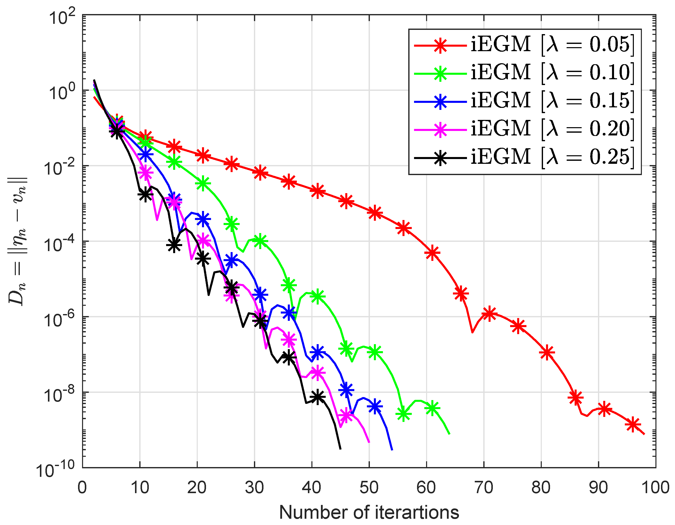
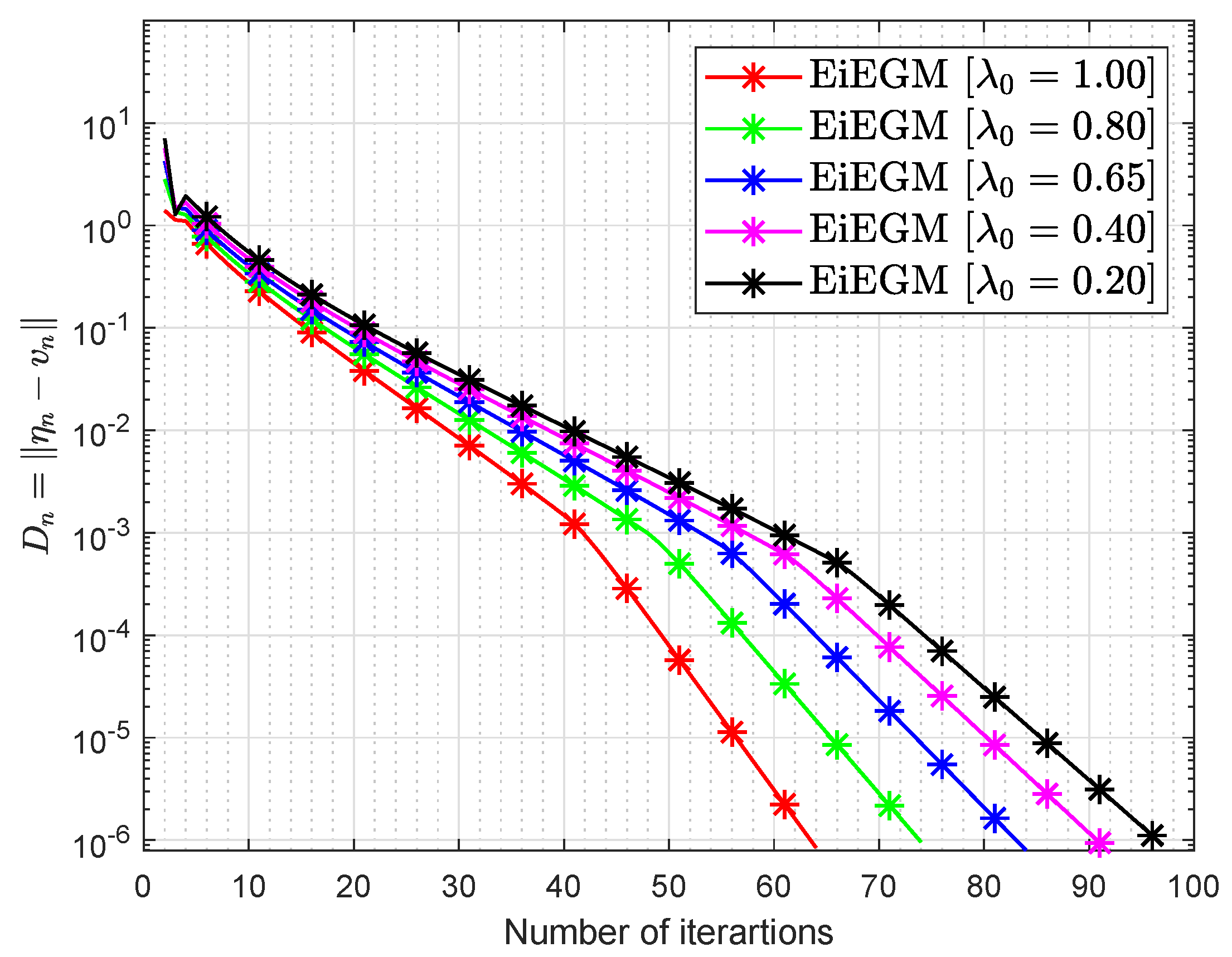
while Lipschitz constants $c_1=c_2=\frac{1}{2}\parallel A-B\parallel$ (see for more details [7,46,47]). The set $\mathcal{C}\subset {\mathcal{R}}^5$ is $\mathcal{C}:=\{u\in {\mathcal{R}}^5:-5\le u_i\le 5\}.$ Figure 1 and Figure 2 and Table 3 report the numerical results by choosing $u_{-1}=u_0=(1,\cdots ,1),$ $\mu =0.33$ and $ϵ={10}^{-6}.$

Figure 1. Example 2: numerical behavior of Algorithm 3.1 in [39] by choosing different values of $\lambda$.

Figure 2. Example 2: numerical behavior of Algorithm 1 by choosing different values of ${\lambda }_0.$

Table 3. Figure 1 and Figure 2: Algorithm 1 numerical comparison with Algorithm 1 in [39].

			Number of Iterations		Execution Time in Seconds
$\mathbf{\vartheta }$	$\mathbf{\lambda }$	${\mathbf{\lambda }}_{\mathbf{0}}$	iEGM	EiEGM	iEGM	EiEGM
0.50	0.05	0.15	98	64	2.2174	1.6342
0.50	0.10	0.35	64	50	1.6815	1.3452
0.50	0.15	0.55	54	46	1.5712	1.2011
0.50	0.20	0.75	50	42	1.5196	1.0845
0.50	0.25	0.95	45	38	1.3859	1.0023

Example 3.

Let $f(\breve{p},\breve{q})=⟨F\left(\breve{p}\right),\breve{q}-\breve{p}⟩$ and $F\left(\breve{p}\right)=G\left(\breve{p}\right)+H\left(\breve{p}\right),$ where

$$G\left(\breve{p}\right)=\left(g_1\left(\breve{p}\right),g_2\left(\breve{p}\right),\cdots ,g_n\left(\breve{p}\right)\right),H\left(\breve{p}\right)=E\breve{p}+c,c=(-1,-1,\cdots ,-1)$$

and

$$g_i\left(\breve{p}\right)={\breve{p}}_{i-1}^2+{\breve{p}}_i^2+{\breve{p}}_{i-1}{\breve{p}}_i+{\breve{p}}_i{\breve{p}}_{i+1},i=1,2,\cdots ,n,{\breve{p}}_0={\breve{p}}_{n+1}=0.$$

The entries of a square matrix E are taken in the following way:

$$e_{i,j}=\left\{\begin{array}{cc}4\hfill & j=i\hfill \\ 1\hfill & i-j=1\hfill \\ -2\hfill & i-j=-1\hfill \\ 0\hfill & otherwise,\hfill \end{array}\right.$$

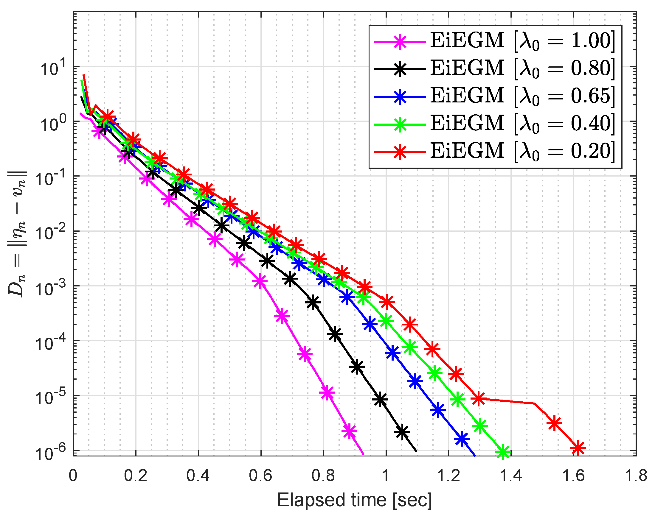
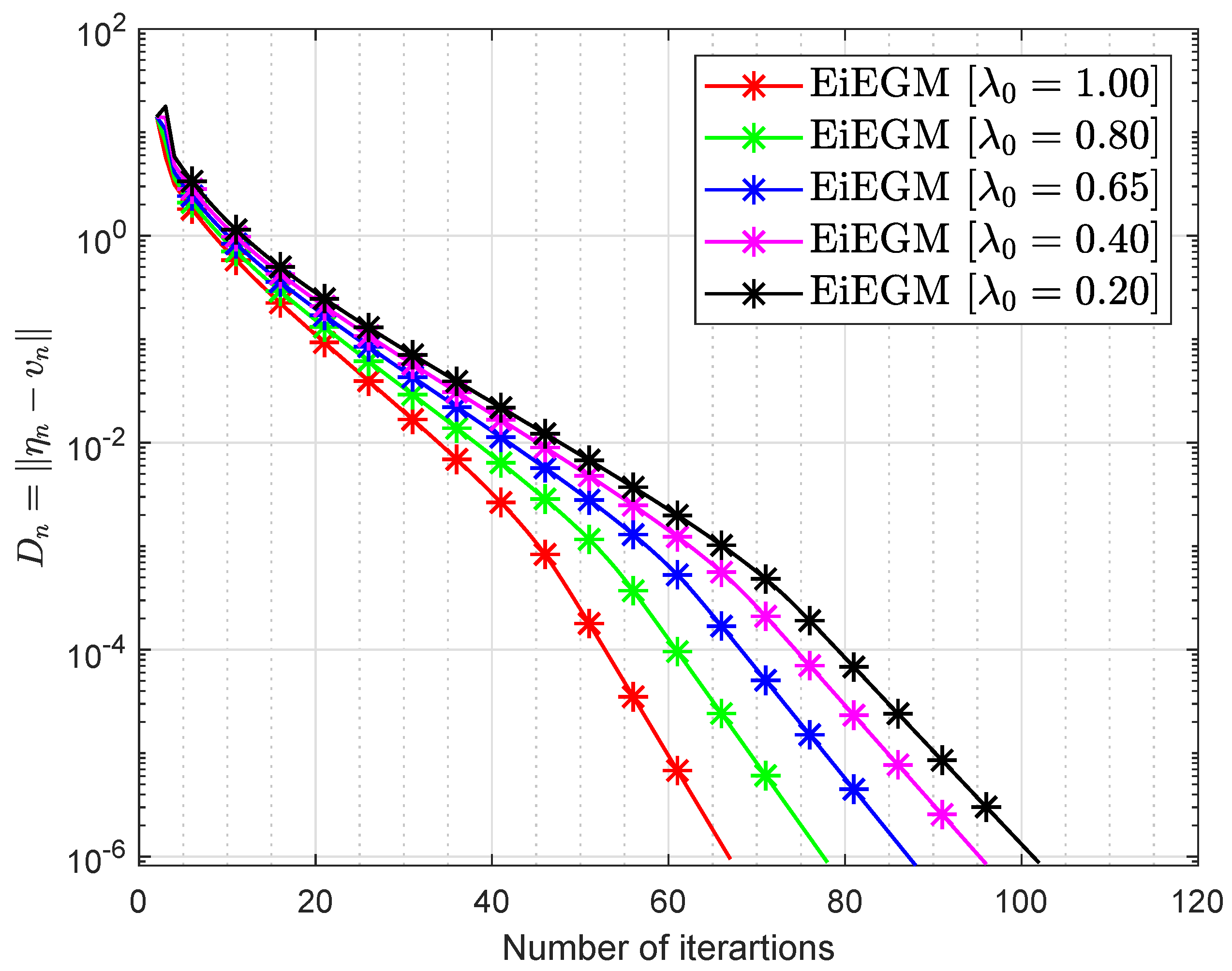
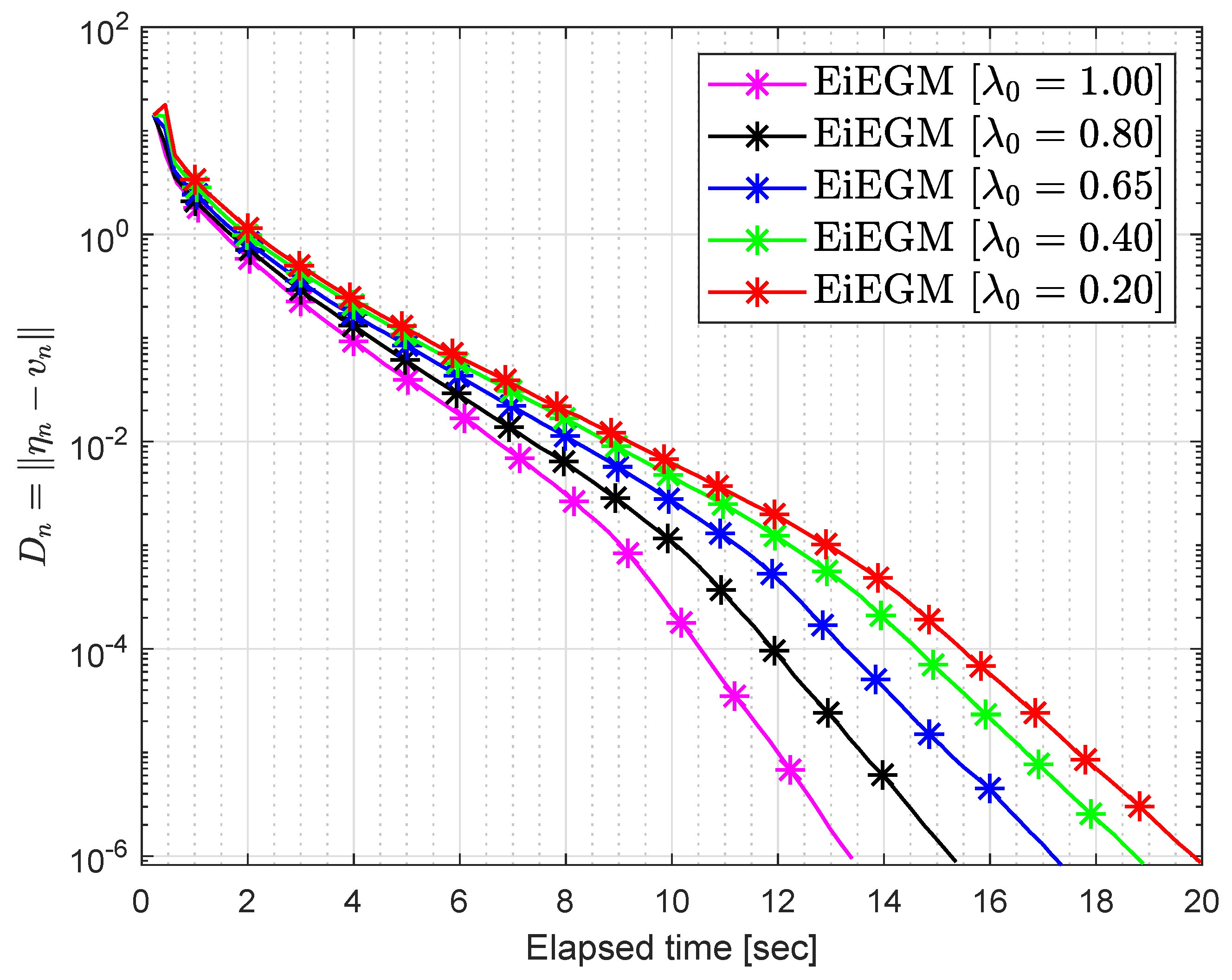
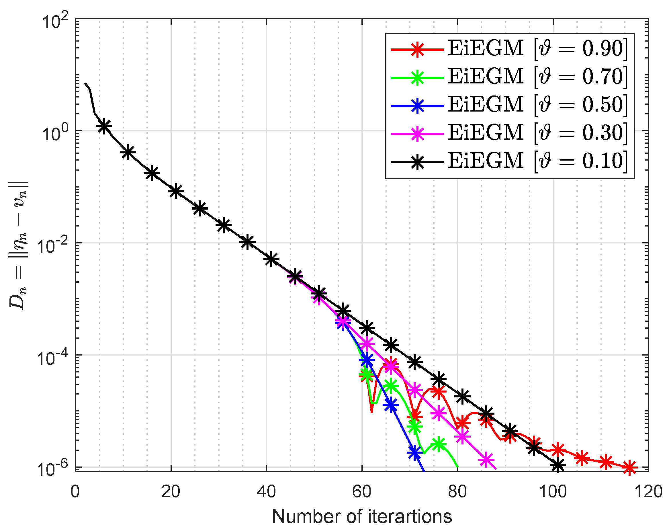
where $\mathcal{C}=\left\{(u_1,\cdots ,u_n)\in {\mathcal{R}}^n:u_i\ge 1,i=2,\cdots ,n\right\}.$ To see the optimum values of the control parameters, some experiments were carried out taking into account the variation of the control parameters ${\lambda }_0$ and the inertial factor ϑ. Figure 3, Figure 4, Figure 5, Figure 6, Figure 7 and Figure 8 and Table 4 and Table 5 report the numerical results by choosing $u_{-1}=u_0=(1,\cdots ,1),$ $\mu =0.33$ and $ϵ={10}^{-6}.$

Figure 3. Numerical conduct of Algorithm 1 in ${\mathcal{R}}^{50}$ by choosing different values of ${\lambda }_0.$

Figure 4. Numerical conduct of Algorithm 1 in ${\mathcal{R}}^{50}$ by choosing different values of ${\lambda }_0.$

Figure 5. Numerical conduct of Algorithm 1 in ${\mathcal{R}}^{200}$ by choosing different values of ${\lambda }_0.$

Figure 6. Numerical conduct of Algorithm 1 in ${\mathcal{R}}^{200}$ by choosing different values of ${\lambda }_0.$

Figure 7. Numerical conduct of Algorithm 1 in ${\mathcal{R}}^{50}$ by choosing different values of $\vartheta .$

Figure 8. Numerical conduct of Algorithm 1 in ${\mathcal{R}}^{50}$ by choosing different values of $\vartheta .$

Table 4. Numerical results for Algorithm 1 in ${\mathcal{R}}^{50}$ by choosing different values of ${\lambda }_0$ and $\vartheta .$

	EiEGM		EiEGM
${\mathbf{\lambda }}_{\mathbf{0}}$	Number of Iterations	CPU Time	$\mathbf{\vartheta }$	Number of Iterations	Execution Time
1.00	64	0.9276	0.90	116	1.8066
0.80	74	1.0975	0.70	80	1.2464
0.60	84	1.2849	0.50	73	1.1262
0.40	91	1.3740	0.30	88	1.3788
0.20	97	1.6298	0.10	102	1.6159

Table 5. Numerical results for Algorithm 1 in ${\mathcal{R}}^{200}$ by choosing different values of ${\lambda }_0$ and $\vartheta .$

	EiEGM		EiEGM
${\mathbf{\lambda }}_{\mathbf{0}}$	Number of Iterations	CPU Time	$\mathbf{\vartheta }$	Number of Iterations	Execution Time
1.00	67	13.3967	0.90	105	20.6972
0.80	78	15.3566	0.70	80	15.5770
0.60	88	17.3471	0.50	80	15.4838
0.40	96	18.8894	0.30	94	19.4532
0.20	102	19.9705	0.10	108	21.9745

Example 4.

Suppose that $\mathcal{H}=L^2\left([0,1]\right)$ is a Hilbert space with an inner product $⟨u,v⟩={\int }_0^{1}u\left(t\right)v\left(t\right)dt,\forall u,v\in \mathcal{H}$ and the induced norm

$$\parallel u\parallel =\sqrt{{\int }_0^1{\left|u\left(t\right)\right|}^{2}dt}.$$

Assume that $\mathcal{C}:=\{u\in L^2\left([0,1]\right):\parallel u\parallel \le 1\}$ is the unit ball. Let $K:\mathcal{C}\to \mathcal{H}$ be

$$K\left(u\right)\left(t\right)={\int }_0^1\left(u\left(t\right)-H(t,s)f\left(u\right(s\left)\right)\right)ds+g\left(t\right),$$

where

$$H(t,s)=\frac{2ts{e}^{(t+s)}}{e\sqrt{e^2-1}},f\left(u\right)=cosx,g\left(t\right)=\frac{2t{e}^t}{e\sqrt{e^2-1}}.$$

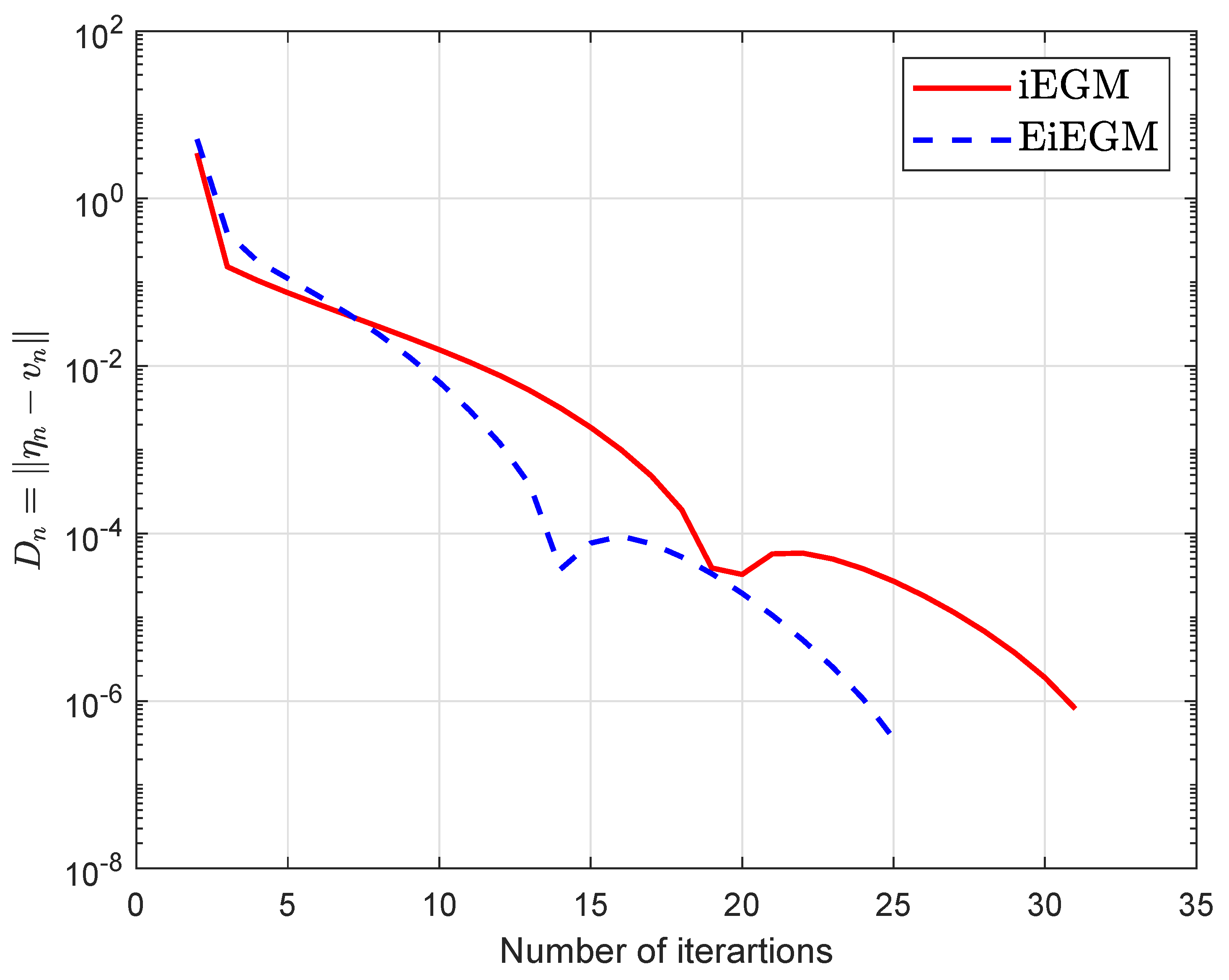
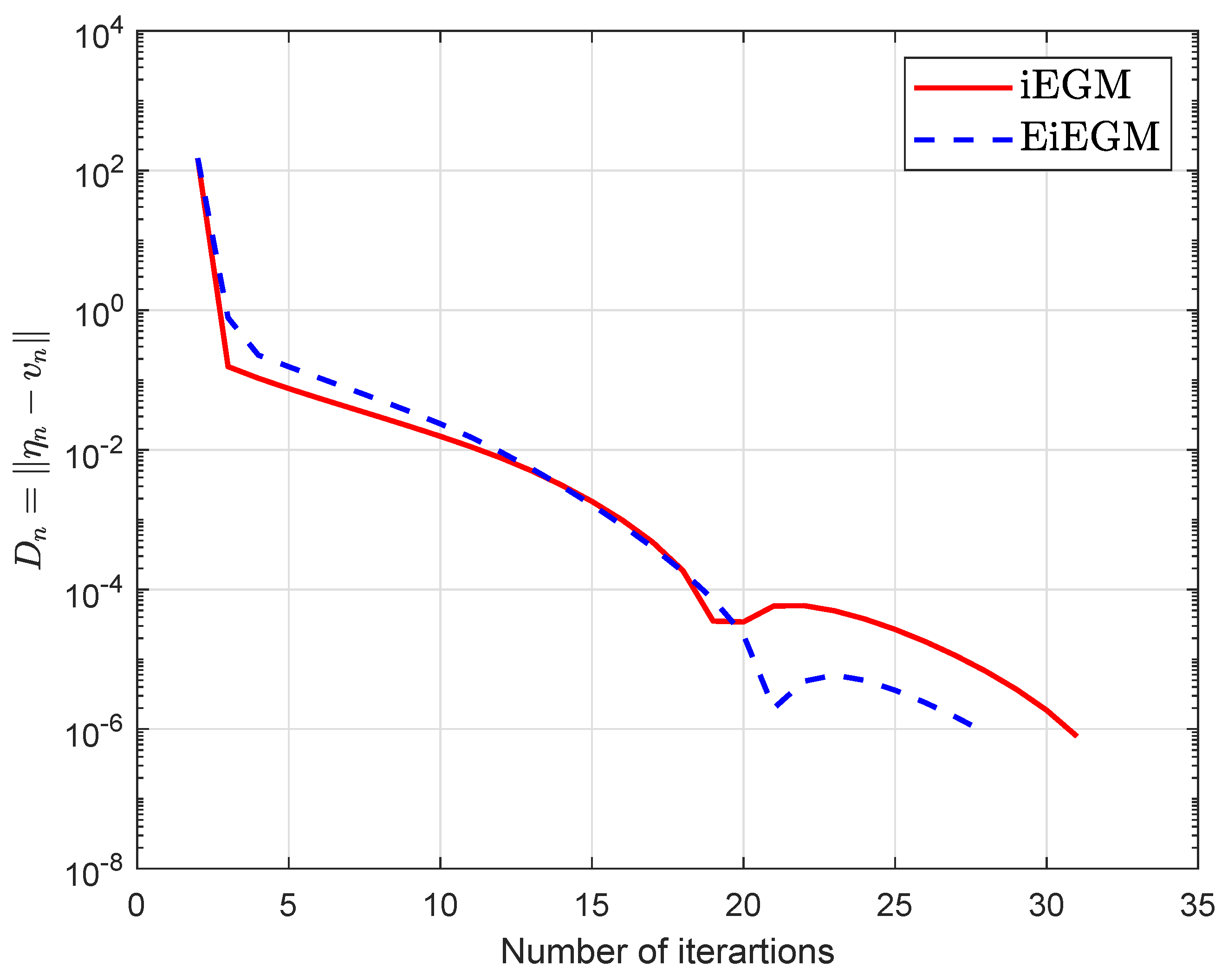
We can see in [48] that K is monotone and Lipschitz-continuous with a Lipschitz constant of $L=2$. Figure 9 and Figure 10 and Table 6 show the numerical results by choosing different values of $u_0$ and $ϵ={10}^{-6}.$

Figure 9. Algorithm 1 comparison with Algorithm 1 in [39] by choosing values of $u_{-1}=u_0=1.$

Figure 10. Algorithm 1 comparison with Algorithm 1 in [39] by choosing values of $u_{-1}=u_0=t.$

Table 6. Example 4: numerical comparison of Algorithm 1 with Algorithm 1 in [39].

				Number of Iterations		Execution Time in Seconds
${\mathit{u}}_{-\mathbf{1}}={\mathit{u}}_{\mathbf{0}}$	$\mathbf{\vartheta }$	$\mathbf{\lambda }$	${\mathbf{\lambda }}_{\mathbf{0}}$	iEGM	EiEGM	iEGM	EiEGM
1	0.50	0.20	0.50	31	25	0.0158	0.0158
t	0.50	0.20	0.50	31	27	0.0158	0.0158
$2t^2$	0.50	0.20	0.50	33	30	0.0158	0.0158
$sin\left(t\right)$	0.50	0.20	0.50	37	30	0.0158	0.0158
$exp\left(t\right)$	0.50	0.20	0.50	42	32	0.0158	0.0158

Discussion on the Numerical Experiments: We have the following findings about the above-mentioned experiments:

(1)

The proposed Algorithm 1 does not depend on the Lipschitz constants, unlike Algorithm 1 in [39]. Algorithm 1 uses a variable stepsize that is updated for each iteration and depends on some of the previous iterations. The key advantage of Algorithm 1 is that it works without prior knowledge of the Lipschitz-type constants $c_1$ and $c_2,$ unlike Algorithm 1 in [39].

(2)

Four examples were discussed to compare our proposed method with Algorithm 1 in [39]. In particular, information on Lipschitz constants is missing in Example 3. Due to the missing information of the Lipschitz constants we cannot run Algorithm 1 in [39] because the stepsize $\lambda$ is dependent on Lipschitz constants, i.e., $0<\lambda <min\{\frac{1}{2c_1},\frac{1}{2c_2}\}.$ However, we can use the proposed Algorithm 1 to solve Example 3.

(3)

It is noted that the selection of the $\vartheta$ value is always important, and precisely the value $\vartheta \in (3,6)$ is better than most other values.

(4)

Choosing of the ${\lambda }_0$ value is critical and the proposed algorithm performs better when ${\lambda }_0$ is closer to $1.$

(5)

It can also be acknowledged that the efficiency of an algorithms significantly depends on the nature of the problem and tolerance. More time and a considerable number of iterations are needed for large-scale problems. In this case, we could see that a certain stepsize value improves the efficiency of the algorithm and improves the convergence rate.

(6)

Figure 9 and Figure 10 and Table 6 suggest that the choice of initial points and the complexity of the bifunction have an effect on the performance of algorithms in terms of number of iterations and time elapsed.

References

1. Blum, E. From optimization and variational inequalities to equilibrium problems. Math. Stud. 1994, 63, 123–145. [Google Scholar]
2. Bianchi, M.; Schaible, S. Generalized monotone bifunctions and equilibrium problems. J. Optim. Theory Appl. 1996, 90, 31–43. [Google Scholar] [CrossRef]
3. Fan, K. A Minimax Inequality and Applications, Inequalities III; Shisha, O., Ed.; Academic Press: New York, NY, USA, 1972. [Google Scholar]
4. Facchinei, F.; Pang, J.S. Finite-Dimensional Variational Inequalities and Complementarity Problems; Springer Science & Business Media: Berlin, Germany, 2007. [Google Scholar]
5. Konnov, I. Equilibrium Models and Variational Inequalities; Elsevier: Amsterdam, The Netherlands, 2007; Volume 210. [Google Scholar]
6. Muu, L.D.; Oettli, W. Convergence of an adaptive penalty scheme for finding constrained equilibria. Nonlinear Anal. Theory Methods Appl. 1992, 18, 1159–1166. [Google Scholar] [CrossRef]
7. Quoc Tran, D.; Le Dung, M.N.V.H. Extragradient algorithms extended to equilibrium problems. Optimization 2008, 57, 749–776. [Google Scholar] [CrossRef]
8. Ur Rehman, H.; Kumam, P.; Cho, Y.J.; Yordsorn, P. Weak convergence of explicit extragradient algorithms for solving equilibirum problems. J. Inequalities Appl. 2019, 2019. [Google Scholar] [CrossRef]
9. Quoc, T.D.; Anh, P.N.; Muu, L.D. Dual extragradient algorithms extended to equilibrium problems. J. Glob. Optim. 2011, 52, 139–159. [Google Scholar] [CrossRef]
10. Lyashko, S.I.; Semenov, V.V. A new two-step proximal algorithm of solving the problem of equilibrium programming. In Optimization and Its Applications in Control and Data Sciences; Springer International Publishing: Berlin/Heidelberg, Germany, 2016; pp. 315–325. [Google Scholar] [CrossRef]
11. Takahashi, S.; Takahashi, W. Viscosity approximation methods for equilibrium problems and fixed point problems in Hilbert spaces. J. Math. Anal. Appl. 2007, 331, 506–515. [Google Scholar] [CrossRef] [Green Version]
12. Ur Rehman, H.; Kumam, P.; Je Cho, Y.; Suleiman, Y.I.; Kumam, W. Modified Popov’s explicit iterative algorithms for solving pseudomonotone equilibrium problems. Optim. Methods Softw. 2020, 1–32. [Google Scholar] [CrossRef]
13. Anh, P.N.; Hai, T.N.; Tuan, P.M. On ergodic algorithms for equilibrium problems. J. Glob. Optim. 2015, 64, 179–195. [Google Scholar] [CrossRef]
14. Hieu, D.V.; Quy, P.K.; Vy, L.V. Explicit iterative algorithms for solving equilibrium problems. Calcolo 2019, 56. [Google Scholar] [CrossRef]
15. Hieu, D.V. New extragradient method for a class of equilibrium problems in Hilbert spaces. Appl. Anal. 2017, 97, 811–824. [Google Scholar] [CrossRef]
16. Ur Rehman, H.; Kumam, P.; Abubakar, A.B.; Cho, Y.J. The extragradient algorithm with inertial effects extended to equilibrium problems. Comput. Appl. Math. 2020, 39. [Google Scholar] [CrossRef]
17. Santos, P.; Scheimberg, S. An inexact subgradient algorithm for equilibrium problems. Comput. Appl. Math. 2011, 30, 91–107. [Google Scholar]
18. Ur Rehman, H.; Kumam, P.; Kumam, W.; Shutaywi, M.; Jirakitpuwapat, W. The inertial sub-gradient extra-gradient method for a class of pseudo-monotone equilibrium problems. Symmetry 2020, 12, 463. [Google Scholar] [CrossRef] [Green Version]
19. Hieu, D.V. Halpern subgradient extragradient method extended to equilibrium problems. Rev. Real Acad. Cienc. Exactas Físicas y Nat. Ser. A Matemáticas 2016, 111, 823–840. [Google Scholar] [CrossRef]
20. Anh, P.N.; An, L.T.H. The subgradient extragradient method extended to equilibrium problems. Optimization 2012, 64, 225–248. [Google Scholar] [CrossRef]
21. Ur Rehman, H.; Kumam, P.; Argyros, I.K.; Deebani, W.; Kumam, W. Inertial extra-gradient method for solving a family of strongly pseudomonotone equilibrium problems in real Hilbert spaces with application in variational inequality problem. Symmetry 2020, 12, 503. [Google Scholar] [CrossRef] [Green Version]
22. Muu, L.D.; Quoc, T.D. Regularization algorithms for solving monotone Ky Fan inequalities with application to a Nash-Cournot equilibrium model. J. Optim. Theory Appl. 2009, 142, 185–204. [Google Scholar] [CrossRef]
23. Ur Rehman, H.; Kumam, P.; Argyros, I.K.; Alreshidi, N.A.; Kumam, W.; Jirakitpuwapat, W. A self-adaptive extra-gradient methods for a family of pseudomonotone equilibrium programming with application in different classes of variational inequality problems. Symmetry 2020, 12, 523. [Google Scholar] [CrossRef] [Green Version]
24. Ur Rehman, H.; Kumam, P.; Argyros, I.K.; Shutaywi, M.; Shah, Z. Optimization based methods for solving the equilibrium problems with applications in variational inequality problems and solution of Nash equilibrium models. Mathematics 2020, 8, 822. [Google Scholar] [CrossRef]
25. Ur Rehman, H.; Kumam, P.; Shutaywi, M.; Alreshidi, N.A.; Kumam, W. Inertial optimization based two-step methods for solving equilibrium problems with applications in variational inequality problems and growth control equilibrium models. Energies 2020, 13, 3292. [Google Scholar] [CrossRef]
26. Gibali, A.; Hieu, D.V. A new inertial double-projection method for solving variational inequalities. J. Fixed Point Theory Appl. 2019, 21. [Google Scholar] [CrossRef]
27. Thong, D.V.; Hieu, D.V. Modified subgradient extragradient method for variational inequality problems. Numer. Algorithms 2017, 79, 597–610. [Google Scholar] [CrossRef]
28. Thong, D.V.; Hieu, D.V. Inertial extragradient algorithms for strongly pseudomonotone variational inequalities. J. Comput. Appl. Math. 2018, 341, 80–98. [Google Scholar] [CrossRef]
29. Censor, Y.; Gibali, A.; Reich, S. Extensions of Korpelevich’s extragradient method for the variational inequality problem in Euclidean space. Optimization 2012, 61, 1119–1132. [Google Scholar] [CrossRef]
30. Yordsorn, P.; Kumam, P.; Rehman, H.U. Modified two-step extragradient method for solving the pseudomonotone equilibrium programming in a real Hilbert space. Carpathian J. Math. 2020, 36, 313–330. [Google Scholar]
31. Hammad, H.A.; ur Rehman, H.; la Sen, M.D. Advanced algorithms and common solutions to variational inequalities. Symmetry 2020, 12, 1198. [Google Scholar] [CrossRef]
32. Gibali, A. A new non-Lipschitzian projection method for solving variational inequalities in Euclidean spaces. J. Nonlinear Anal. Optim. Theory Appl. 2015, 6, 41–51. [Google Scholar]
33. Dong, Q.L.; Jiang, D.; Gibali, A. A modified subgradient extragradient method for solving the variational inequality problem. Numer. Algorithms 2018, 79, 927–940. [Google Scholar] [CrossRef] [Green Version]
34. Abubakar, J.; Kumam, P.; ur Rehman, H.; Ibrahim, A.H. Inertial iterative schemes with variable step sizes for variational inequality problem involving pseudomonotone operator. Mathematics 2020, 8, 609. [Google Scholar] [CrossRef]
35. Abubakar, J.; Sombut, K.; ur Rehman, H.; Ibrahim, A.H. An accelerated subgradient extragradient algorithm for strongly pseudomonotone variational inequality problems. Thai J. Math. 2019, 18. [Google Scholar]
36. Flåm, S.D.; Antipin, A.S. Equilibrium programming using proximal-like algorithms. Math. Program. 1996, 78, 29–41. [Google Scholar] [CrossRef]
37. Korpelevich, G. The extragradient method for finding saddle points and other problems. Matecon 1976, 12, 747–756. [Google Scholar]
38. Yang, J.; Liu, H.; Liu, Z. Modified subgradient extragradient algorithms for solving monotone variational inequalities. Optimization 2018, 67, 2247–2258. [Google Scholar] [CrossRef]
39. Vinh, N.T.; Muu, L.D. Inertial extragradient algorithms for solving equilibrium problems. Acta Math. Vietnam. 2019, 44, 639–663. [Google Scholar] [CrossRef]
40. Censor, Y.; Gibali, A.; Reich, S. The subgradient extragradient method for solving variational inequalities in Hilbert space. J. Optim. Theory Appl. 2010, 148, 318–335. [Google Scholar] [CrossRef] [PubMed] [Green Version]
41. Kreyszig, E. Introductory Functional Analysis with Applications, 1st ed.; Wiley: New York, NY, USA, 1989. [Google Scholar]
42. Tiel, J.V. Convex Analysis: An Introductory Text, 1st ed.; Wiley: New York, NY, USA, 1984. [Google Scholar]
43. Opial, Z. Weak convergence of the sequence of successive approximations for nonexpansive mappings. Bull. Am. Math. Soc. 1967, 73, 591–598. [Google Scholar] [CrossRef] [Green Version]
44. Tan, K.; Xu, H. Approximating Fixed Points of Nonexpansive Mappings by the Ishikawa Iteration Process. J. Math. Anal. Appl. 1993, 178, 301–308. [Google Scholar] [CrossRef] [Green Version]
45. Browder, F.; Petryshyn, W. Construction of fixed points of nonlinear mappings in Hilbert space. J. Math. Anal. Appl. 1967, 20, 197–228. [Google Scholar] [CrossRef] [Green Version]
46. Ur Rehman, H.; Pakkaranang, N.; Hussain, A.; Wairojjana, N. A modified extra-gradient method for a family of strongly pseudomonotone equilibrium problems in real Hilbert spaces. J. Math. Comput. Sci. 2020, 22, 38–48. [Google Scholar] [CrossRef]
47. Yordsorn, P.; Kumam, P.; ur Rehman, H.; Ibrahim, A.H. A weak convergence self-adaptive method for solving pseudomonotone equilibrium problems in a real Hilbert space. Mathematics 2020, 8, 1165. [Google Scholar] [CrossRef]
48. Van Hieu, D.; Anh, P.K.; Muu, L.D. Modified hybrid projection methods for finding common solutions to variational inequality problems. Comput. Optim. Appl. 2017, 66, 75–96. [Google Scholar] [CrossRef]