Abstract
Based on the symmetrical public transportation network data of Xi’an, China obtained by geographic information system (GIS) technology in 2019, three urban public transportation indexes of walking accessibility, bus accessibility, and metro accessibility were established, and a real estate price prediction model was built by using several machine learning algorithms to predict and analysis the housing price in Xi’an, China. Firstly, the symmetrical road network data and real estate property data of Xi’an were collected and preprocessed, secondly, the spatial syntax theory and distance calculation method were applied to establish three indexes of traffic accessibility; finally, taking the house property data and the calculated traffic accessibility indexes as the characteristic index, the real estate price prediction model of Xi’an was constructed by using the random forest algorithm (RF), lightweight gradient lift algorithm (LGBM), and gradient lifting regression tree algorithm (GBDT). The prediction accuracy of the final model is 89.2% and the root-mean-square error is 1761.84. The results show that the accessibility of bus and metro to some extent represent the convenience of public transportation in different areas of urban space. The higher the accessibility index is, the more convenient the traffic is. The real estate price model has high prediction accuracy and can reflect the real situation of urban real estate price. The importance of the three accessibility features to the real estate price prediction model are nearly more than 20%, which indicates that the accessibility of urban public transportation has an important impact on the change of urban real estate price, and the development of urban public transportation plays an important role in the real estate economy.
1. Introduction
With the rise of China’s house prices, the issue of house price has gradually become the focus of the government, consumers, investors, and academic researchers [1]. In urban development, house price planning is of great significance. When people conduct real estate transactions, most of them are based on field investigation and qualitative analysis, which is limited by the factors of both parties, there is no evaluation standard that can reasonably price the house itself, which will lead to unfair transaction to a certain extent [2]. At present, China’s real estate industry is full of chaos. How to quantitatively evaluate the price of the house and determine the main factors affecting the price of the house has become a big problem [3]. The development of public transport in the city can, to a certain extent, improve the regional economic vitality and promote the development of the real estate economy [4]. Therefore, under the background of big data, how to use massive data to reasonably calculate the characteristic indexes to describe the real operation of public transport and subway in the city, highlight the traffic convenience of urban space area, and then explore the link between real estate economy and urban public transport development needs more in-depth research.
Traffic accessibility refers to the expression of the degree of difficulty for an object to move from one location to another through a certain mode of transportation in urban space. Different modes of travel can be subdivided into different accessibility, such as walking accessibility, bus accessibility. metro accessibility, etc. [5]. Domestic and international scholars’ research on traffic accessibility can be traced back to the 1930s. The classical location theory provides a theoretical basis for accessibility [6]. In 1959, Hansen proposed the gravity model method to define the concept of traffic accessibility scientifically [7]. On the basis of this, the following scholars proposed the time–space barrier model, isoline model, competition model, spatial syntax, and other methods to define the traffic accessibility [8]. In the application of traffic accessibility, in recent years, some researchers have introduced it into real estate economics to measure the impact of traffic facilities on real estate prices. Kangwon et al. based on the metro lines in the main urban area of Seoul, South Korea, built the Metro accessibility with the distance between the residential buildings and the metro, and studied the impact of the metro lines on the price of houses along the line [9]. Taking Beijing as an example, Ming et al. analyzed the impact of accessibility of subway, light rail, and urban rail on land use development, and provided theoretical guidance for urban planning [10]. Deborah et al. calculated the accessibility of public transport and subway in Guangzhou, and introduced it into the land price prediction model, and obtained good prediction accuracy [11]. Mitra et al. studied the value of traffic accessibility in underdeveloped countries and provided suggestions for urban planning of Rajshahi city in Bangladesh [5]. Li et al. took Beijing as an example, analyzed the relationship between subway accessibility and housing prices, and explored the impact of transportation on stabilizing housing prices and promoting residents’ employment [12].
In model selection, in 1928, Waugh studied the price and characteristics of Boston vegetables, proposed the linear function relationship between them, and obtained the earliest Hedonic price model (HPM) [13]. In the 1960s, Lancaster first applied HPM model to the real estate field, analyzed the relationship between user demand, house property characteristics and house price, and believed that all the property characteristics of house included the synthesis of house implied price, which provided a solid theoretical basis for the development and application of HPM in the real estate industry [14]. In 1974, Rosen solved the problem of commodity heterogeneity through HPM and related technologies, and established the technical framework of characteristic price analysis in the real estate market [15]. Li Xinru and others used the logarithmic HPM model to predict and analyze the house price when evaluating the benchmark price of urban land [16]. Gao et al. found that factors including spatial features can improve the accuracy of HPM model [17].
Since the beginning of the 21st century, thanks to the improvement of computer hardware technology and the rapid development of software technology, many machine learning algorithms have emerged in the era of big data. Random forest algorithm (RF), gradient lifting regression tree algorithm (GBDT), and lightweight gradient lift algorithm (LGBM) have very good performance in regression prediction and classification prediction. P. Durganjali et al. took the data set of the Kaggle competition website as an example, respectively constructed the logistic regression model, the stochastic forest model, the decision tree model, etc. to predict the house price, among which the prediction accuracy of the stochastic forest model is as high as 86.5% [18]. Dong Qian et al. applied the RF model to analyze the trend of housing price changes in 16 large and medium-sized cities in China in 2011, but the research scope was too large and the amount of data was too small to obtain further accurate conclusions [19]. Yang Bowen and others used GBDT algorithm and RF algorithm to build house price prediction models based on the house attribute data of California, USA. Although the root mean square error of the model is low and the prediction accuracy is good, it takes a long time to calculate the data and takes up more memory. At the same time, the generalization ability of the experimental results is low due to the small number of samples and feature dimensions [20]. LGBM introduces a histogram acceleration algorithm on the basis of GBDT to ensure a certain prediction accuracy while increasing the speed of the model. Compared with GBDT that needs to load the data set every time it fits the residuals and consumes memory for a long time, LGBM performs better in terms of running time and memory usage. It is very suitable for industrial-grade massive data processing [21]. Although the LGBM model improves the calculation speed and reduces the memory usage, the LGBM model reduces the accuracy of predicting housing prices [22]. Based on the above considerations, in order to improve data computing efficiency, reduce memory usage, and improve housing price prediction accuracy, we merge RF, GBDT, and LGBM, and propose a model fusion model (Stacking) for housing price prediction in Xi’an, China.
Banerjee D and others summarized a variety of machine learning algorithms, and predicted the trend of urban housing prices [23]. Vineeth N and other machine learning algorithms are applied to analyze the house price and its influencing factors [24]. Phan et al. Used machine learning algorithm to predict the trend of house prices based on the historical transaction prices in Melbourne, Australia [25].
In the study of housing price forecasting model, in addition to model selection, we also need to consider characteristic factors. Brueckner et al. analyzed the impact of urban planning related factors under macro policies on real estate prices in 1987 [26]. Evans et al. analyzed the impact on the house price from the surrounding environmental factors such as the surrounding school distribution and public infrastructure construction [27]. Malpezzi mainly studies the impact of commercial economic vitality in urban areas on housing prices [28]. Diaz et al. analyzed the impact of rail transit layout on real estate prices [29]. Wu Wenjie et al. studied the influence of four factors on house price in terms of transportation, life, work convenience, and environmental facility convenience [30].
In this paper, taking Xi’an as an example, by collecting and analyzing the data of housing attributes, urban public transport and subway in Xi’an, the author constructs three kinds of characteristic indexes of house internal attribute factors, location factors, traffic accessibility factors and surrounding environment factors, with 20 kinds of characteristics, constructs the house price prediction model combining with a variety of machine learning algorithms, explores the causes and influencing factors of house price.
2. Materials and Methods
2.1. Data Source
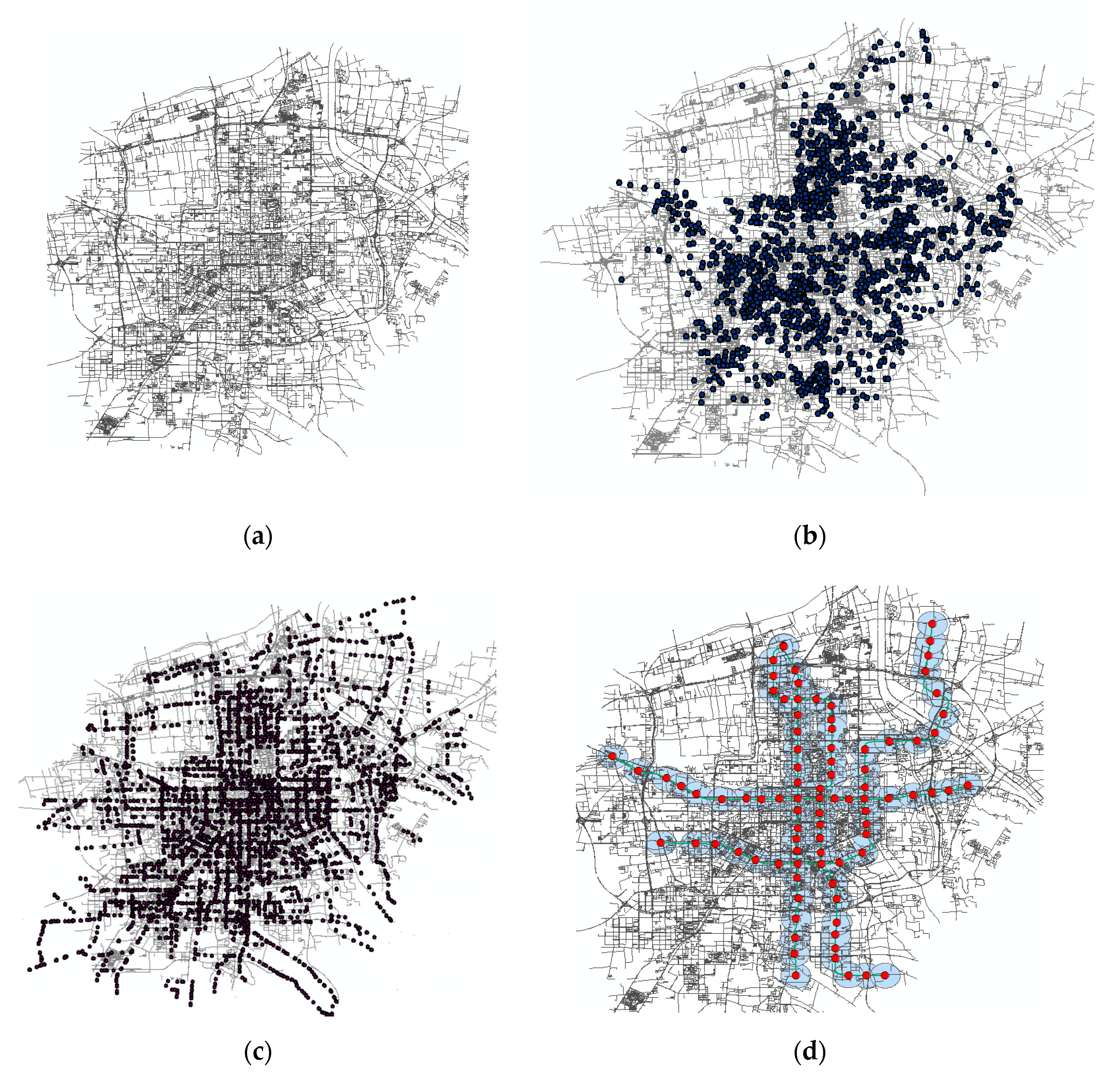
The data source and data composition were described in this chapter. The data source is the house property data, house price data and urban symmetrical traffic data in the main urban area of Xi’an, China. The spatial projection distribution of data in a scalable, comprehensive GIS platform (ArcGIS) software is shown in Figure 1. The main collection method for the house attribute data is to capture the information of Lianjia (a house information publishing website), and the collection time is September 2019. For housing price data, the main collection method is to obtain information from Anjuke (a housing information service platform), and the collection time is September 2019. The data of urban symmetrical basic road network, urban bus and metro of urban symmetrical traffic data are obtained mainly through the application programming interface (API) interface of Gaud map, and the data collection time is August 2019.
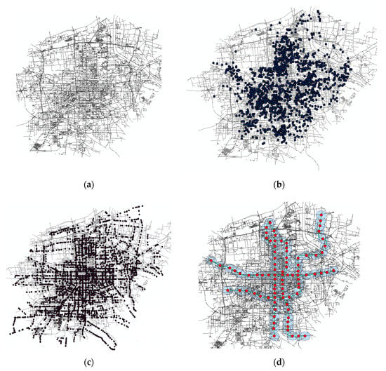
Figure 1.
Data spatial distribution in Xi’an, China. (a) Urban road network spatial distribution. (b) Housing spatial distribution. (c) Bus spatial distribution. (d) Metro spatial distribution.
Figure 1a shows the road network data map of Xi’an City, including urban main roads, auxiliary roads and branch roads. Figure 1b shows the property data of houses in the urban area with the road network as the base map. Figure 1c,d respectively project and mark the bus and metro data of Xi’an city. The acquisition of these data provides data support for the later construction of characteristic indicators.
Xi’an housing attribute data is selected from all the housing attribute data in the main urban area of Xi’an, including the internal attribute data, location data, etc. In this study, the initial housing attribute data collection amount reached 79,452 pieces of data. The amount of data used in this study was 29,180 pieces after removing the duplicate data, error data and missing information data. It provides a huge data support for the subsequent building of house price forecast model and lays a data foundation for the model research by establishing urban housing data table.
Urban traffic data can be divided into three categories: urban basic road network data table, urban bus data table, and urban metro data table. Urban traffic data has such characteristics of large amount and wide range. In this study, in order to collect data of Xi’an road network, the number of road network nodes has reached 210,000, the number of bus stations has reached 21,099, and for the metro data, 89 stations of 4 lines are collected. The collection of these data is mainly to provide data support for the establishment of traffic accessibility indicators in the next section for further analysis and research.
2.2. Analysis Framework
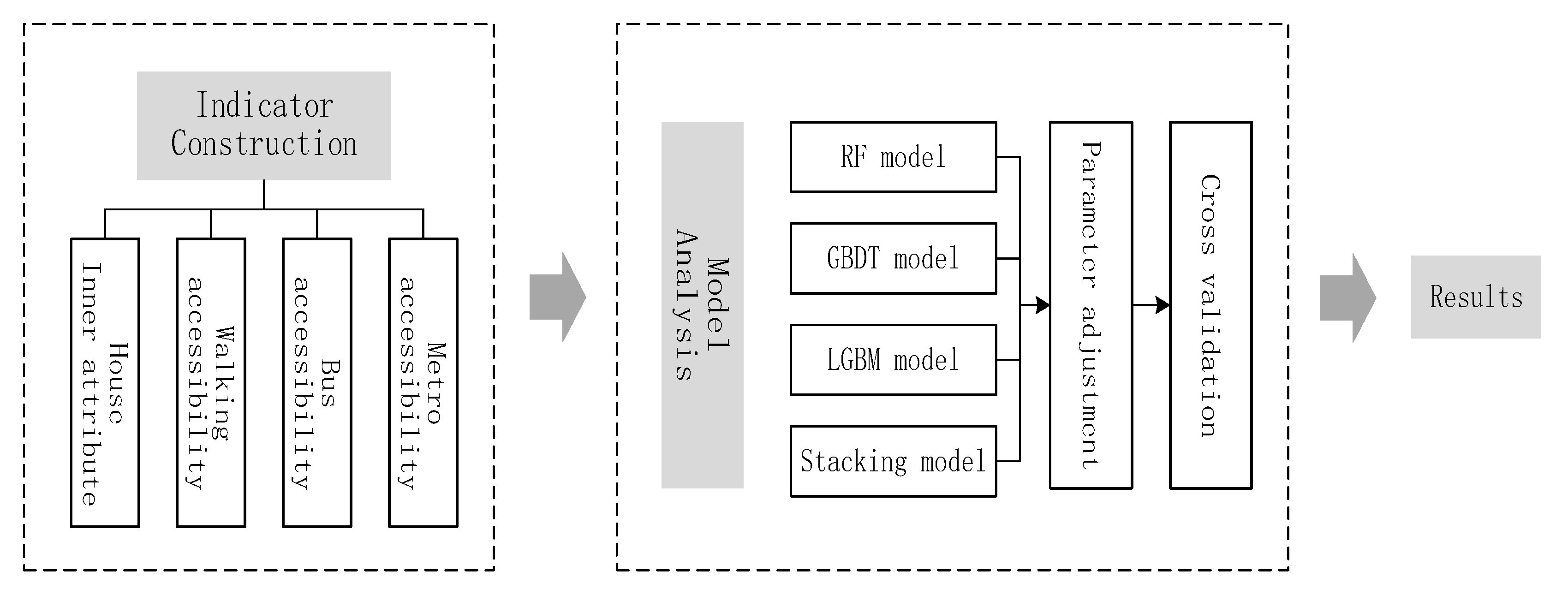
From the flow chart of house price prediction (Figure 2), it can be seen that this method has two advantages: one is to introduce traffic accessibility index, take walking, bus and metro as the carrier of urban spatial network, and analyze the causes of house price in the whole city. The other is to use a variety of machine learning algorithms to build a house price prediction model to ensure the prediction accuracy of the model.
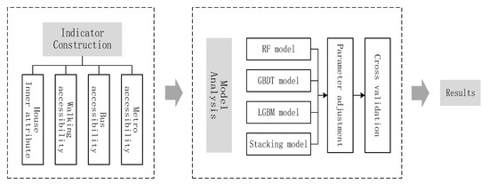
Figure 2.
Flow chart of housing price prediction.
2.3. Data Processing
This chapter will introduce the related technology and theoretical basis of traffic accessibility, as well as the traffic accessibility evaluation model used in this study. Traffic accessibility refers to the degree of traffic convenience when residents choose different modes of transportation to arrive at the destination from the starting point. Traffic accessibility plays an important role in road network optimization, land use planning, land use evaluation, and location analysis [31]. In this study, three traffic accessibility methods are based on spatial syntax theory.
2.3.1. Walking Accessibility
Walking accessibility reflects the convenience of people walking in the city. It refers to the measurement value of all point-to-point mobile walking in the road network calculated by the space syntax theory when the whole road network is accessible by walking.
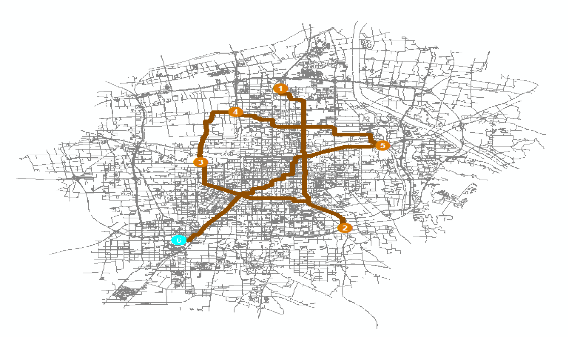
First of all, we need to obtain the basic road network map data of Xi’an city. In order to ensure the connectivity of the map, we need to break the line segment. In this paper, we break the line segment according to the distance of 100 m. In addition, we also break the line at the intersection of the road. In this way, all roads in Xi’an are connected. Next, the network topology of road network map is carried out in ArcGIS software to ensure that any two points on the map can be connected along the road. Figure 3 shows the basic road network and the connected road network after topology in Xi’an.
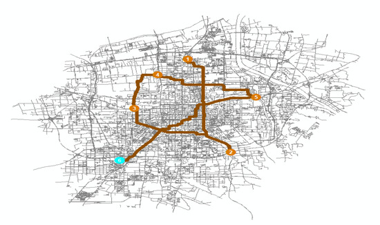
Figure 3.
Topologically connected road network diagram.
In Figure 3, six points are randomly selected on the road network map to solve the problem, and it is found that the path planning along the map route can be achieved. All lines can be connected after the road network is broken. Next, we need to convert the map to an axis map. The operation of this step is completed in Depthmap software (British Space Syntax Ltd), and the transformed axis map is shown in Figure 4.
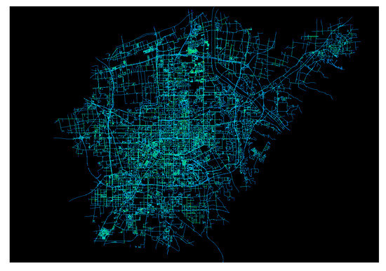
Figure 4.
Axis map of Xi’an.
After the transformation into the axis map, the integration calculation, that is, the walking accessibility calculation is needed. The calculation of walking accessibility is affected by the search radius. In this study, the radius range is selected as 1000–10,000 m, in which every 200 m is calculated. The calculation formula is as follows:
In Equation (1), represents the walking accessibility of node , represents the shortest path distance, and represents the number of summary points in the road network. Finally, the axis map is transformed into road network map, which is imported into ArcGIS software (American environmental systems research institute, Inc.), and the attribute table is opened to get the walking accessibility under different radius. At this time, the calculated pedestrian accessibility index is attached to the road network map of Xi’an city, then we need to associate it with the housing data and determine the optimal radius to get the pedestrian accessibility of each housing location. ArcGIS software will be used to associate the characteristics of pedestrian accessibility and housing data nextly.
Firstly, the road network map of Xi’an city with walking accessibility index is imported into ArcGIS software, and the point type data or line segment type data is transformed into trend surface data by kernel density analysis function, so that the accessibility plane covering the whole road map of Xi’an city can be obtained. Secondly, the accessibility plane is transformed into grid data, and then the grid data is transformed into point data to prepare for neighbor analysis. Finally, the grid turning point data and the house attribute data are analyzed in the neighborhood, and the walking accessibility indexes under different radii are related to the house attribute data table to get the walking accessibility characteristics of different radii under each house location.
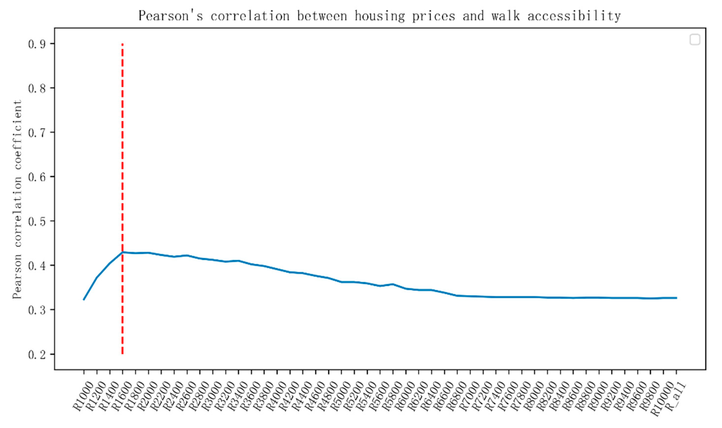
In the above calculation, there are several groups of walking accessibility values under different search radius, so it is necessary to determine the optimal search radius. In this paper, the Pearson correlation coefficient between house price and walking accessibility is calculated to judge, and the highest coefficient is selected as the best search radius and walking accessibility. In statistics, Pearson correlation coefficient is used to measure the degree of correlation between two groups of variables [32]. The calculation formula is shown in Equation (2). Figure 5 shows Pearson correlation coefficient between house price and pedestrian accessibility based on spatial syntax under different radius of pedestrian accessibility.

Figure 5.
Pearson correlation coefficient graph of house price and walk accessibility under different radii.
In Equation (2), is Pearson correlation coefficient of and variables, is total sample, and are sample mean, and is the standard deviation of the sample.
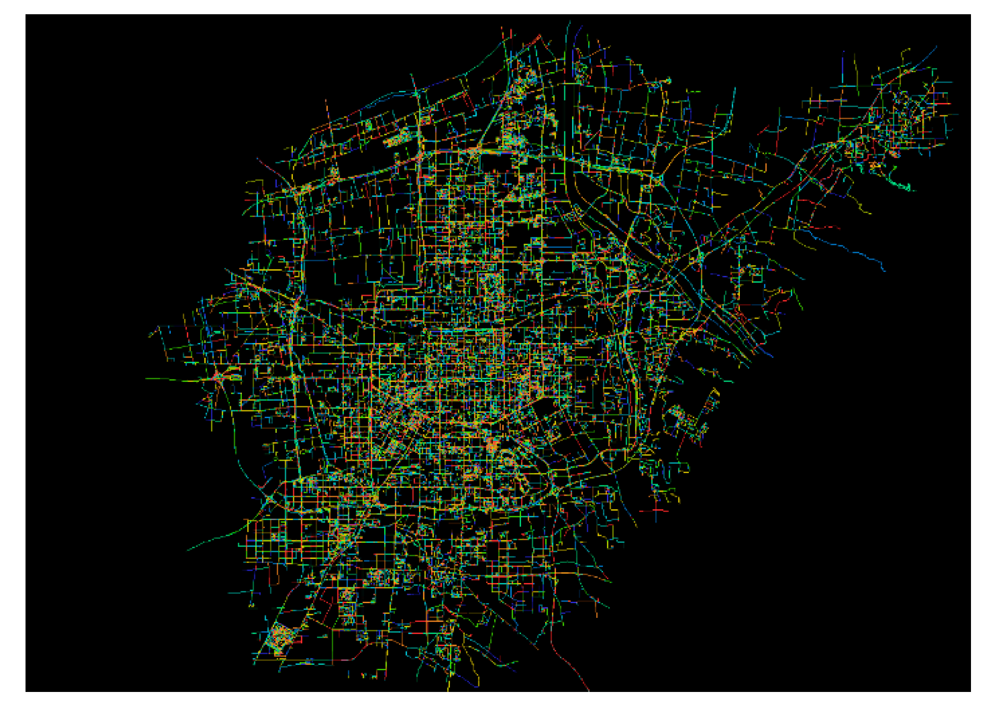
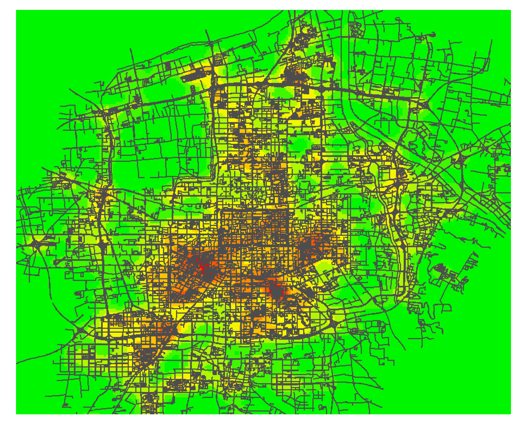
In Figure 5, the accessibility under the highest radius of Pearson correlation coefficient is selected, and the best search radius for pedestrian accessibility is determined as = 1600 m. Figure 6 shows the axis diagram under space syntax calculation when = 1600 m. The pedestrian accessibility under this radius is retained as the optimal pedestrian accessibility feature of the house. Figure 7 shows the heat distribution map of Xi’an road network axis and pedestrian accessibility when the search radius is = 1600 m.
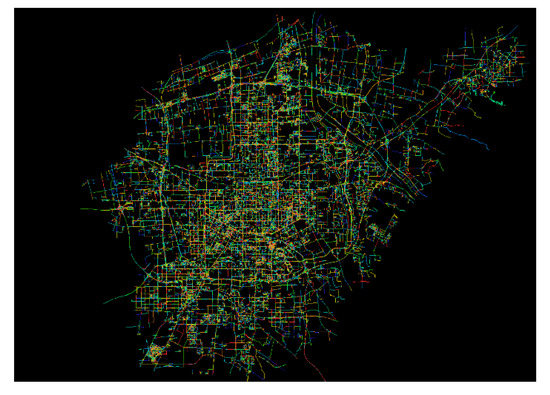
Figure 6.
Axis map of Xi’an road network.
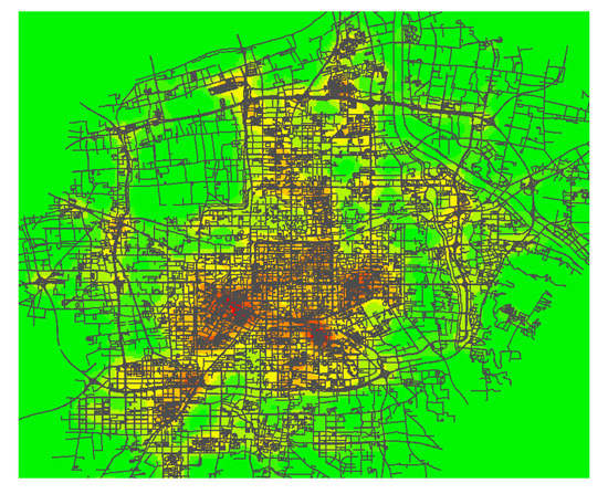
Figure 7.
Thermal map of walk accessibility.
2.3.2. Bus Accessibility
The bus accessibility based on spatial syntax refers to the measurement value of the connectivity of bus stations in urban road network by combining the spatial syntax theory. The calculation method of bus accessibility and walking accessibility is similar.
Firstly, the road network map of Xi’an city and the collected bus station data are merged in ArcGIS software, and the intersection of bus station and road network is used as the road node to break the road network and reconstruct the network topology. Secondly, transform the map into an axis map to calculate the integration degree under different search radius. The radius range is 1000–10,000 m, and calculate every 200 m. Next, the axis map is imported into ArcGIS inverted, and then the number of lines at each bus station is assigned as the weight. Finally, the bus accessibility of each bus station under different search radius is obtained. The calculation formula of public transport accessibility is shown in Equation (3).
In Equation (3), is the bus accessibility of node , represents the shortest path distance between two bus stations, and represents the number of bus stations in the road network. represents the number of bus lines at station . In this paper, the definition of bus accessibility, because no specific bus line operation diagram is obtained, can only be replaced by the basic road network, so there is no way to accurately calculate the real route between the station and station, use the shortest distance of the road network to replace.
At this time, we get that the bus accessibility under different radius is attached to bus station, and then we need to associate these features with the urban housing features. The association mode is the same as that in the previous section. Firstly, the calculated data of Xi’an bus station with bus accessibility index is imported into ArcGIS software, and the core density analysis function is applied to convert the point type data into trend surface data, so that the bus accessibility plane covering the whole Xi’an urban area can be obtained. Secondly, the accessibility plane is transformed into grid data, and then transform the grid data into point data to prepare for neighbor analysis. Finally, the grid turning point data and the house attribute data are analyzed in ArcGIS, and the bus accessibility indexes under different radii are related to the house attribute data table to get the bus accessibility characteristics of different radii under each house location.
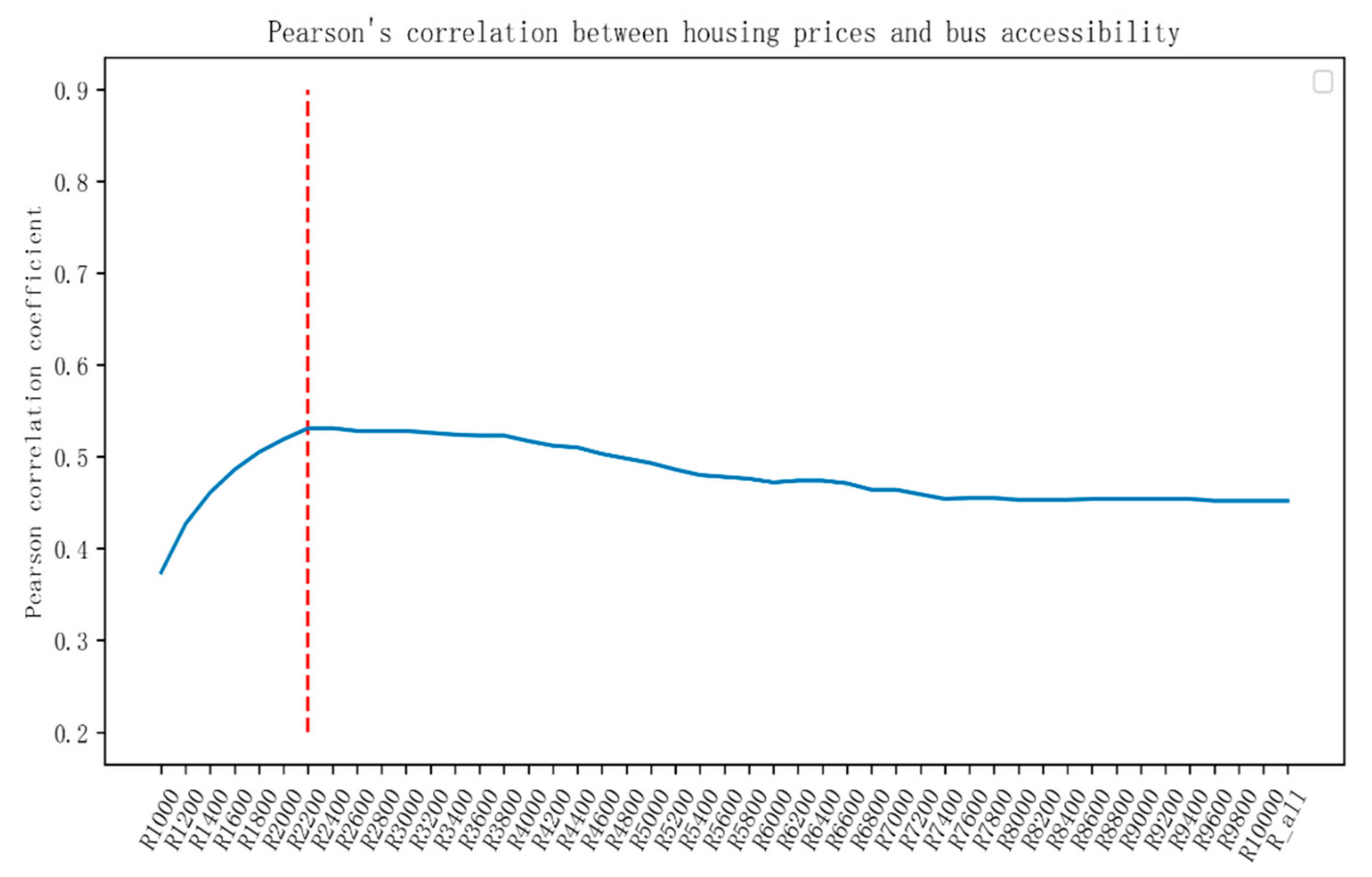
Next, we still need to analyze and determine the bus accessibility under the optimal radius. The Pearson correlation analysis method is still used to calculate the Pearson correlation coefficient between the house price and the bus accessibility under different radius, and the maximum coefficient is taken as the bus accessibility under the optimal radius. Figure 8 shows Pearson correlation coefficient of house price and bus accessibility under different radius.

Figure 8.
Pearson correlation coefficient graph of house price and bus accessibility under different radii.
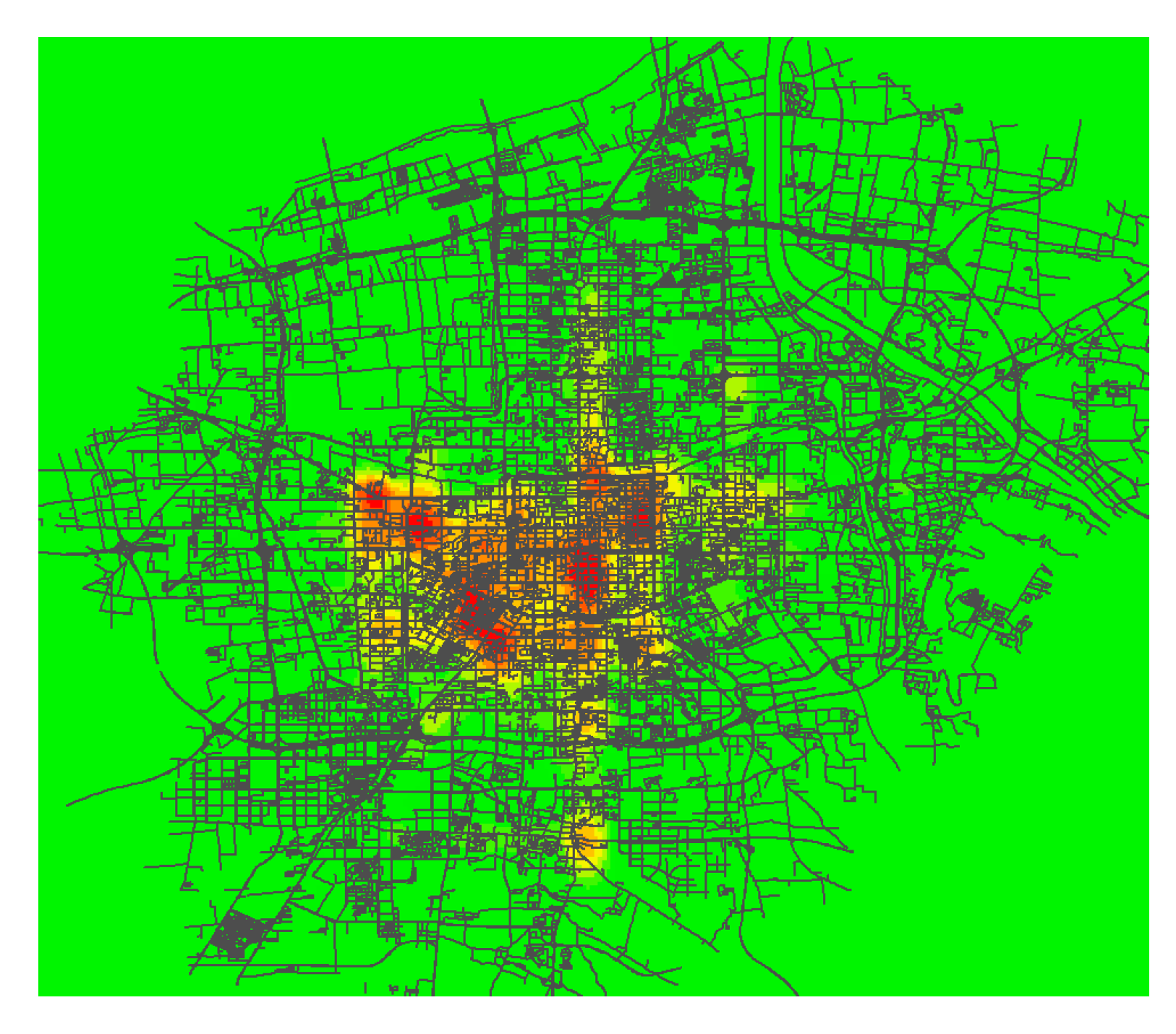
In Figure 8, select the bus accessibility under the highest radius of Pearson correlation coefficient, and then determine the best search radius of bus accessibility as = 2200 m. Therefore, the bus accessibility under this radius is retained as the optimal bus accessibility feature of the house. Figure 9 shows the thermal distribution of bus accessibility in Xi’an when the search radius is = 2200 m.
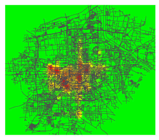
Figure 9.
Thermal map of bus accessibility.
2.3.3. Metro Accessibility
The metro accessibility based on spatial syntax is calculated based on Xi’an subway line map and station data, combined with spatial syntax theory. The calculation process is similar to walking accessibility and bus accessibility.
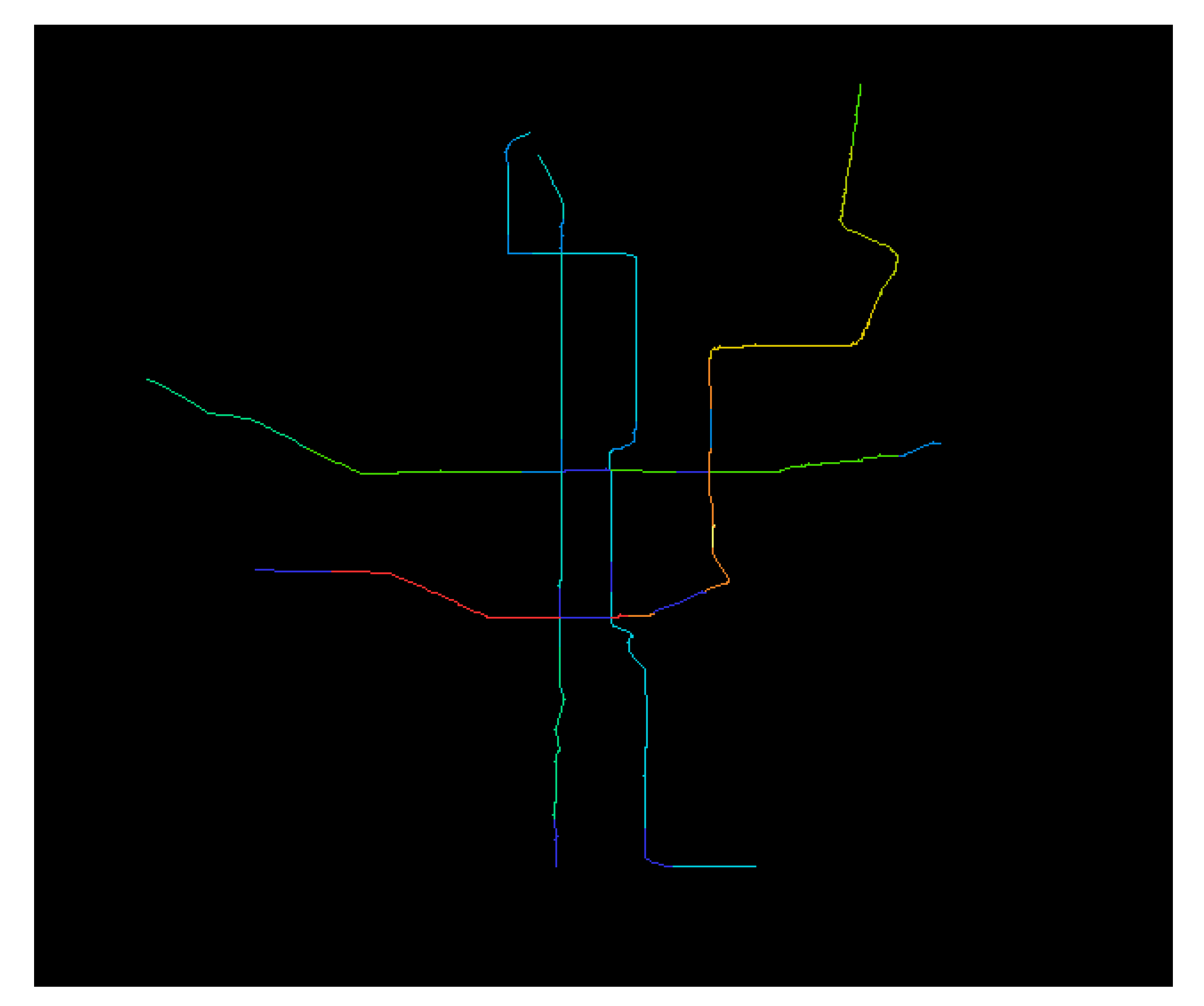
Firstly, the Xi’an subway line map is broken at the station, and the connectivity map is obtained after network topology. Then transform it into an axis map, and the integration degree under different radii is calculated in the Depthmap software, the radius range is 1000–10,000 m and the global range and the calculation interval is 200 m once. Next, import the inverse transformation of the axis map with the integration degree calculation into ArcGIS. Figure 10 shows the metro axis under the global calculation integration. The calculation results of other radii are similar. Finally, the metro accessibility of each station under different search radius is obtained.

Figure 10.
Axis map of metro lines.
As can be seen in Figure 10, the distribution of the axis map does not conform to the accessibility distribution of metro lines in subjective experience. The accessibility should be higher at the passenger and exchange stations of the four lines, and the integration degree cannot truly reflect the subway accessibility. It is considered to distinguish the transfer station from the common station and give different weight values. Therefore, after the integration degree is calculated, converted back the axis map to the original map and opened in ArcGIS, the integration degree attribute value of each metro station will be obtained. Assign the weight of the station again, and the weight is the number of transfer lines at the station. The metro accessibility under different radius of subway station is obtained. The calculation formula is shown in Equation (4).
In Equation (4), represents the metro accessibility of node , represents the running distance between two metro stations, and represents the number of metro stations in the road network. refers to the number of transfer lines at station .
Like walking accessibility and bus accessibility, metro accessibility also needs to be related to house price characteristics, and the method of association still uses the nearest neighbor analysis function in ArcGIS. Firstly, import the calculated data of Xi’an public transport station with metro accessibility index into ArcGIS software, and apply the core density analysis function is to convert the point type data into trend surface data, so that the metro accessibility plane covering the whole Xi’an urban area can be obtained. Secondly, transform the accessibility plane into grid data, and then transform the grid data into point data to prepare for neighbor analysis. Finally, the grid turning point data and the house attribute data are analyzed in ArcGIS, and the metro accessibility indexes under different radii are related to the house attribute data table to get the metro accessibility characteristics of different radii under each house location.
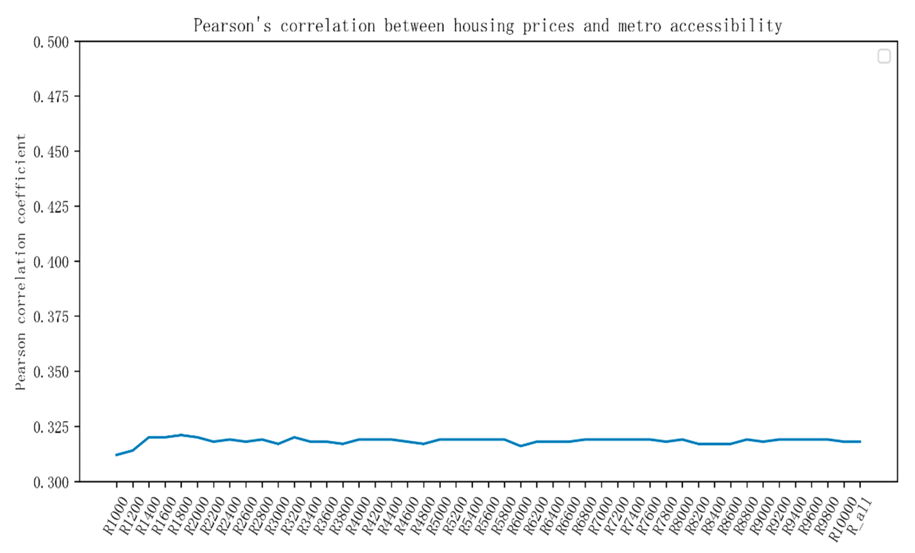
Next, we need to determine the optimal search radius. Figure 11 shows Pearson correlation coefficient of house price and metro accessibility under different radii. Select the radius with the largest coefficient as the best radius.
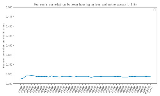
Figure 11.
Pearson correlation coefficient graph of house price and metro accessibility under different radii.
It can be seen from Figure 11 that the Pearson correlation coefficient of subway accessibility and house price is stably distributed with low value, which basically does not change with the change of radius which is because there are fewer subway lines and the distribution of interval distance between stations is average, which is not as complex as road network and bus station, so the change is small. At present, Xi’an has only opened four lines, which cannot completely cover the whole urban space. Most of the houses are far away from the subway station, so Pearson correlation value is low. In this paper, the global scope is selected as the final metro accessibility index.
3. Experimental Results
The walking accessibility, bus accessibility, and metro accessibility indexes are related to the house property form, and the data used to analyze the house price are obtained. Using the RF, GDBT, LGBM, and Stacking algorithms of machine learning algorithm to build the housing price prediction model. First of all, divide the data set into two groups, one group takes the traffic accessibility calculated by the spatial syntax theory as the traffic characteristic index. Second, the two groups of data sets are respectively applied to four machine learning algorithms to build the housing price prediction model, and the optimal model is selected through five indexes, including the prediction accuracy R², root mean square error RMSE, model volume, model training time, and prediction time. Finally, the optimal models under the two sets of data are compared and analyzed to determine the merits of the traffic accessibility calculation, and the final housing price prediction model is determined, which provides the model basis for the subsequent application research.
3.1. Real Estate Price Estimation for RF
The process of building a real estate price prediction model based on the random forest algorithm (RF) is: firstly, the training set data is put into the model, and adjust the parameters of random forest. Secondly, K-fold cross validation is introduced to judge whether the model is over fitted, and the average validation accuracy and error of the model are obtained. Finally, save the model, and the price is predicted with the test set data to get the prediction accuracy of the model. Among them, Equations (5) and (6) are used to evaluate the accuracy and error of the model.
represents the number of samples; represents the real value of the sample; represents the predicted value of the sample; and represents the mean value of the samples. is used to measure the prediction accuracy of the algorithm model, the closer the value is to 0, the more inaccurate it is, and the closer the value is to 1, the more accurate it is. RMSE is the root mean square error, and the smaller the value is, the better the model is.
First, adjust the model parameters. In the RF algorithm, the mesh parameters of n_estimators and max_features are adjusted, and the other parameters are the default values. Based on RMSE, the parameter adjustment diagram is shown in Figure 12.
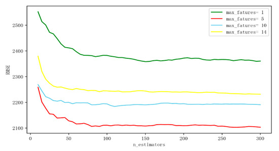
Figure 12.
Parameter adjustment diagram of random forest algorithm (RF) model.
In Figure 12, the abscissa represents the number of trees in the random forest, and the ordinate represents the root mean square error. It can be seen that the error tends to be stable when the n_estimators is greater than 150, and the effect of the model is better when the max_features = 5. Therefore, n_estimators = 150 and max_features = 5 are selected as the fixed parameters of the RF model.
Secondly, K-fold Cross Validation is used in the process of model parameter adjustment to prevent model over fitting. In this paper, K = 10 is selected, and the training set is randomly divided into 10 parts. 9 of them are taken as the training set each time, and the remaining 1 is taken as the verification set. After training the model for 10 times, the training accuracy and root mean square error of 10 times are shown in Table 1 below.

Table 1.
Results of RF algorithm with K-fold Cross Validation.
According to the results in Table 1, in the 10 verifications of the model, there is no obvious low prediction accuracy, and the average prediction accuracy of the model reaches 0.8852. This shows that it has a good prediction ability, and there is no over fitting. Therefore, the current trained RF model is used as the housing price prediction model, and the model is saved.
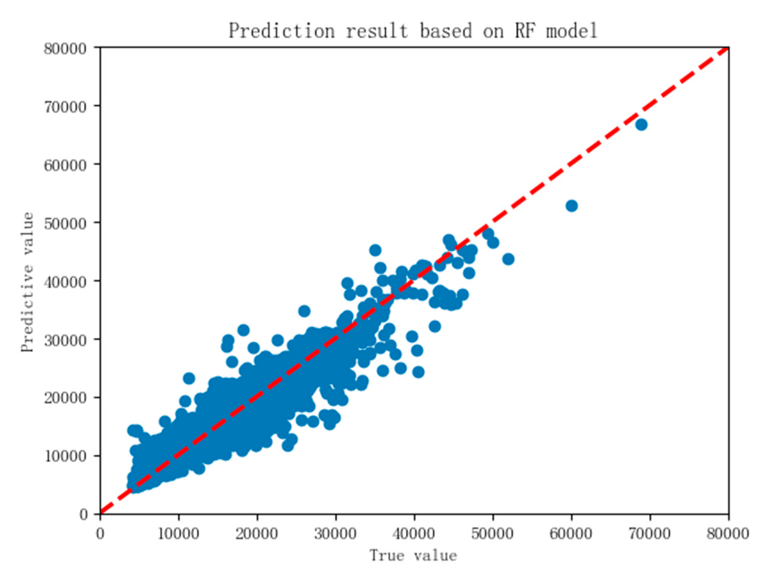
Finally, the RF model is tested with 30% of the test set data separated in advance, because the test set data does not participate in the model training at all, the data results have certain objectivity. Put the test set data into the RF housing price prediction model, and the final scatter diagram of the prediction results is shown in Figure 13, the R² score is 0.891 and the RMSE is 1776.79.

Figure 13.
Scatterplot of RF house price prediction.
In Figure 13, the abscissa represents the real value of the house price, and the ordinate represents the predicted value of the house price. When the point distribution is closer to the center line, the closer the predicted value is to the real value, the smaller the error between them is, and the higher the prediction accuracy of the model is. From the prediction results, when the house price is less than 25,000, the points have a good distribution, concentrated near the middle line, and the prediction results are very good. When the house price is more than 30,000, the distribution of points is relatively discrete, which shows that the prediction results are general, which is due to the fact that the data of high house price in the sample is relatively small. From the whole point of view, the points are basically distributed along the diagonal, which shows that the predicted value is not much different from the real value, and the prediction result of the model on the test set is good.
3.2. Real Estate Price Estimation for GBDT
The process of building house price prediction model based on gradient lifting regression tree algorithm (GBDT) is similar to that of random forest. It is also divided into three parts: parameter adjustment, cross validation and result prediction. There are three parameters to be adjusted in this model, namely n_estimators, max_features, and learning_rate. The method of parameter adjustment is the same as that of random forest. Finalize n_estimators = 46, max_features = 15, learning_rate = 0.5, the model has the best performance. At the same time, through the K-fold Cross Validation, the model is judged to be over fitted, and the results under the cross validation are shown in Table 2.

Table 2.
Results of the gradient lifting regression tree algorithm (GBDT) with K-fold Cross Validation.
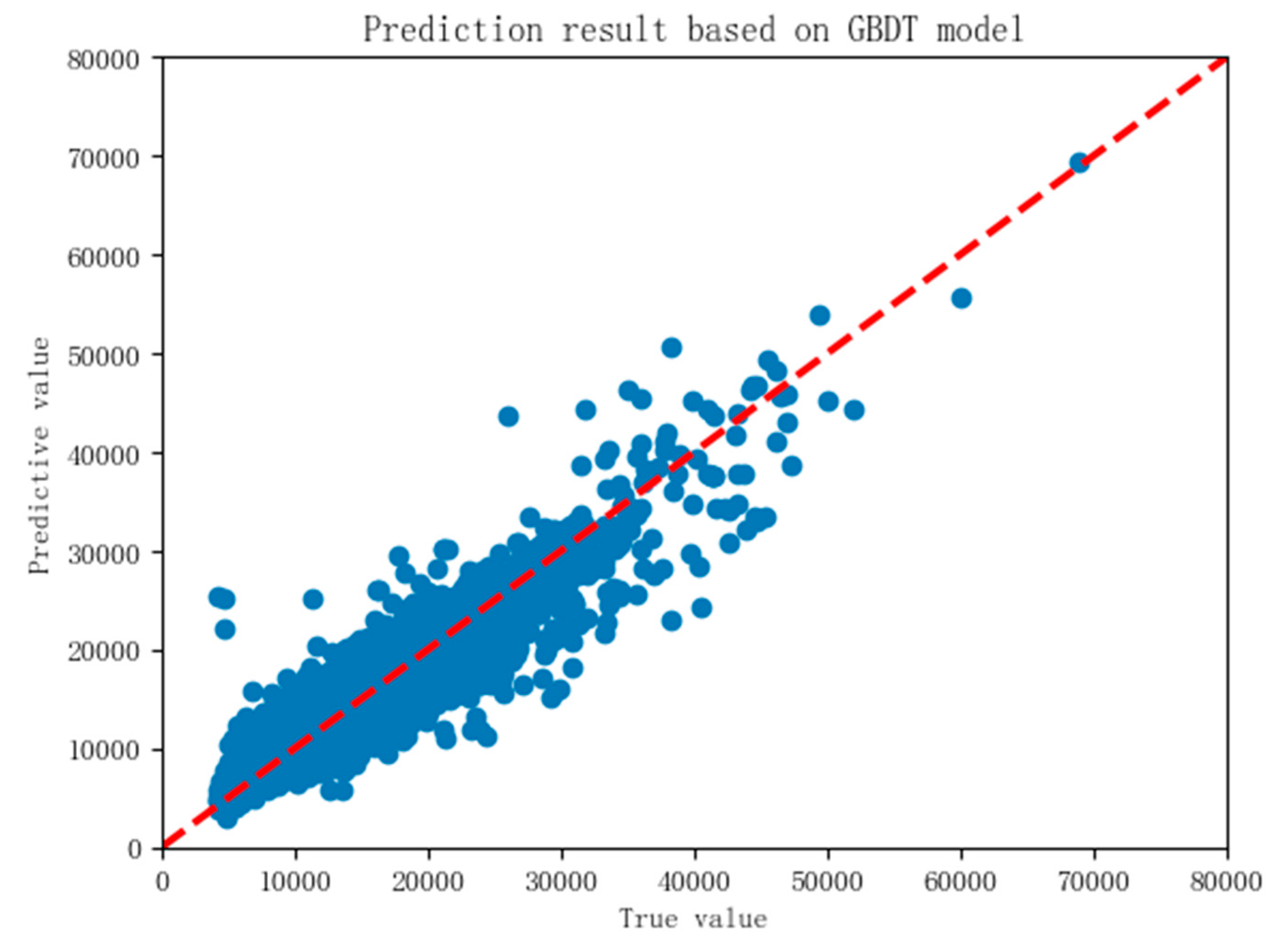
According to the results in Table 2, in the 10 verifications of GBDT model, there is no obvious case of low prediction accuracy, and the average prediction accuracy of the model has reached 0.8632. This shows that it has a good prediction ability, and there is no over fitting. Therefore, the current trained GBDT model is used as the housing price prediction model, and save the model. Finally, the price prediction model based on GBDT algorithm is used to predict the test set data. The predicted results are shown in Figure 14. The R² score is 0.863 and the RMSE is 1979.78.

Figure 14.
Scatterplot of GBDT house price prediction.
In Figure 14, scattered points are basically distributed along the middle line, showing a “shuttle” shape, which shows that GBDT algorithm can make a good prediction of house price. However, from the perspective of model accuracy, GBDT is not as good as RF in predicting housing prices.
3.3. Real Estate Price Estimation for LGBM
The building process of the housing price prediction model based on lightweight gradient lift algorithm (LGBM) is to adjust the parameters first. The three parameters to be adjusted are n_estimators, feature_fraction, and learning_rate, the rest of the parameters use the default value. After adjusting the parameters by the grid parameter adjustment method, it is found that when n_estimators = 350, feature_fraction = 0.25, learning_rate = 0.1, the model performs best. The next step is K-fold Cross Validation. The validation results are shown in Table 3 below.

Table 3.
Results of the lightweight gradient lift algorithm (LGBM) with K-fold Cross Validation.
According to the results in Table 3, the price prediction model based on LGBM has not been fitted, and the average prediction accuracy for the validation set is 0.8503, which is inferior to RF and GBDT models. Next, send the test set into the model for prediction, and the predicted results are shown in Figure 15. The R² score was 0.873 and the RMSE was 1912.71.
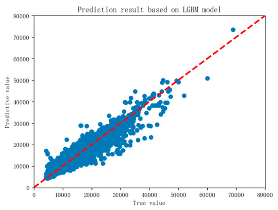
Figure 15.
Scatterplot of LGBM house price prediction.
It can be seen from Figure 15 that the prediction result of the model is good, slightly lower than that of RF. In terms of accuracy and error, it deviates from the researcher’s prediction.
3.4. Real Estate Price Estimation for Stacking
When building the housing price prediction model of stacking algorithm, we need to determine the number of building layers, basic learners, and meta learners. In this paper, we used a two-tier model, and take RF, GBDT, and LGBM as the basic learners, and multiple linear regression as the meta learners to build the housing price prediction model.
Because the first three models are fused, the parameters of the model follow the previous results. Table 4 shows the results of Stacking algorithm under K-fold (K = 10) Cross Validation.

Table 4.
Results of stacking algorithm with K-fold Cross Validation.
According to the results in Table 4, the housing price prediction model based on Stacking has not been fitted, and it performs well for the prediction of the validation set. After saving the model, because the meta model is encapsulated by multiple linear regression equation, the function expression is obtained as shown in Equation (7).
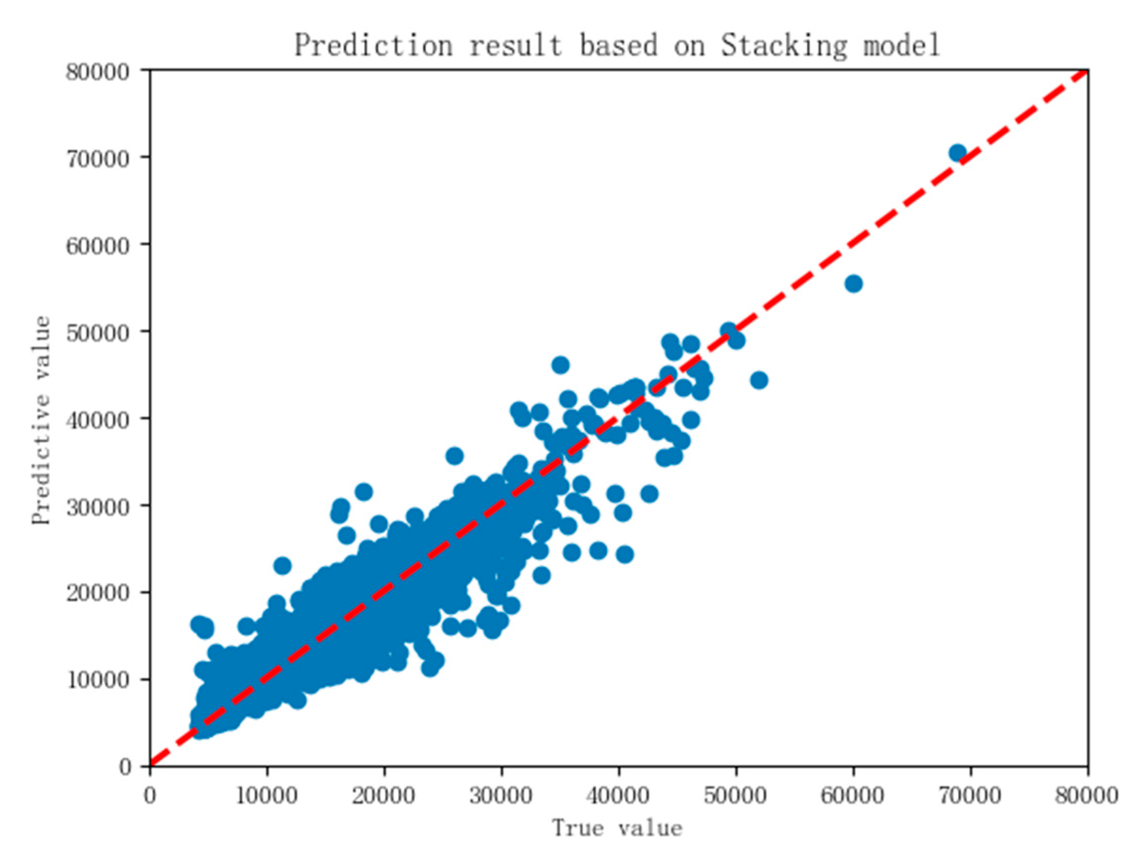
In Equation (7), represents the housing price predicted by the Stacking algorithm, represents the predicted value of RF model, represents the predicted value of GBDT model, and represents the predicted value of LGBM model. In the formula, the input features have the same dimension, so their coefficients can be considered as the proportion of each model in the Stacking algorithm. The model is used to predict the test set data. The forecast results are shown in Figure 16 below, where the R²score is 0.892 and RMSE is 1761.84.

Figure 16.
Scatterplot of stacking house price prediction.
According to the prediction results in Figure 16, the accuracy of housing price prediction model based on stacking is significantly higher than that of GBDT and LGBM single model, slightly higher than that of RF, and the error is lower. The performance of the model is better, which shows that the model stacking method can improve the accuracy of the model to a certain extent. However, in the process of model building, it takes longer.
3.5. Model Comparison
In the previous research, four kinds of house price prediction models are built according to RF algorithm, GBDT algorithm, GBDT algorithm and Stacking algorithm. Then, four models will be compared and analyzed to determine the optimal housing price prediction model. Next, we will make a comparative analysis from five aspects: model accuracy, model error, model scale, model training time, and model running time. Table 5 shows the comparison of various effects of four models. Among them, model size refers to the space size of the generated model. Model training time refers to the time that each model uses 20,426 pieces of training data to build a model. Model running time refers to the time taken to predict 8754 test set data with the model.

Table 5.
Comparison of Model Effect.
In terms of model prediction accuracy and error, Stacking algorithm is superior to the other three, but in terms of real-time performance of model operation, because Stacking algorithm integrates the other three models, the complexity of the model is higher, so the real-time performance is very poor. The prediction accuracy of LGBM algorithm is slightly lower than that of Stacking algorithm, better than RF and GBDT algorithm, and it is the best in real-time performance. In practical application, although the prediction accuracy is important, but also we need to ensure the real-time prediction, so we can consider the housing price prediction model based on RF algorithm. In this paper, the analysis of housing price is still in the stage of theoretical research, it need to better ensure the accuracy of the model, so finally choose the housing price prediction model based on the stacking algorithm as the final model of the follow-up study.
4. Discussion
Although 3.5 determines the best housing price prediction model, and also proves the superiority of calculating traffic accessibility through spatial syntax, however in order to better explore the impact of traffic on housing price, the content of this section will analyze the common characteristics of the model based on the proportion of the characteristics of the four types of machine learning algorithms previously determined. Figure 17 shows the importance percentage of each of the 20 features of the four models in the model building process.
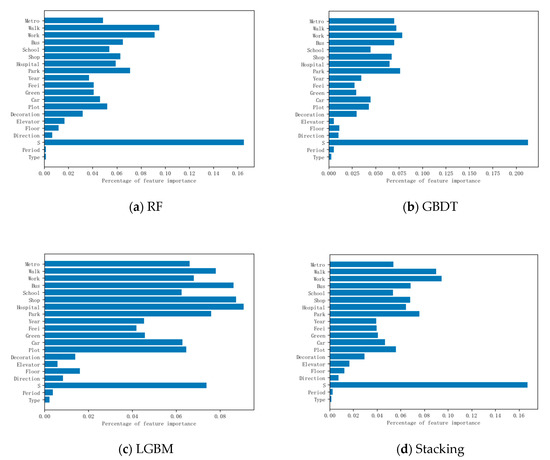
Figure 17.
Importance ratio of the multi-model feature.
It can be found from the characteristic importance proportion in Figure 17 that in the four models, the importance proportion of house area is the largest. In addition, the traffic factors, which are composed of road network accessibility, bus accessibility and metro accessibility calculated by spatial syntax, also account for a large proportion of the importance of the model. After statistics, the proportion of traffic factors in the four models is 21.043%, 20.71%, 22.04%, and 21.68% respectively. This shows that in the housing price analysis, traffic has a great influence on the housing price, which is one of the important factors that cannot be ignored.
To sum up, the spatial syntax theory has more advantages than the simple distance calculation. Three indexes, pedestrian accessibility, public transportation accessibility, and subway accessibility, which are calculated by space syntax theory, cannot be ignored for the impact of house price, and they play a very important role in the building process of house price prediction model.
5. Conclusions
In this study, three characteristic indexes of walking accessibility, bus accessibility and metro accessibility are calculated, which are introduced into the influencing factors of real estate price, and four machine algorithms are used to predict the real estate price in the whole city, good prediction results have been obtained. The research results show that the traffic accessibility calculated according to the space syntax theory can truly reflect the operation of walking, bus and metro in the city, and accurately represent the convenience of public transport in different areas of the city. The walking accessibility and traffic accessibility are introduced into the housing price prediction analysis, and the prediction accuracy of the model reaches 89.2%, At the same time, the important contribution of traffic accessibility to the model reaches nearly 30%, which shows that urban public transport factors have an important impact on urban housing prices
In the model selection, only the relevant algorithms of machine learning are selected for comparative analysis. In recent years, deep learning, neural network, and other model algorithms have better development. In the follow-up research, more and more extensive algorithms will be considered to build the housing price prediction model.
In the future, the research will be carried out from three aspects: first, a more detailed description of the traffic accessibility index. In this paper, the calculation of the bus accessibility index does not fully reflect the real situation, because the actual operation route data of the bus is not obtained, so it is only replaced by the shortest path. Secondly, it is believed that the factors affecting the real estate price are far more than the 24 features mentioned in the paper, we hoped that more influencing factors can be taken into consideration to further improve the model accuracy and prediction effect. Thirdly, it is hoped that the development of urban public transport can be cross studied with other fields, such as location planning of urban business district, medical treatment, school, etc., to explore more possibilities of urban public transport for promoting the vigorous development of the city.
Author Contributions
C.X., S.L., and Y.J. conceived and designed the experiments; C.X., Q.Z., and Q.L. presented tools and carried out the data analysis; C.X. wrote the paper. Y.J. and S.L. guided and revised the paper. C.X. rewrote and improved the theoretical part. Q.Z. and Q.L. collected the materials and did a lot of format editing work. All authors have read and agreed to the published version of the manuscript.
Funding
This research was funded by the General Program of National Natural Science Foundation of China (NSFC) under Grant No.61603057 and No.60804049. This research was also partially supported by the Natural Science Basic Research Plan in Shaanxi Province of China (Grant no.2020JM-255). This research was supported by Xi’an Science and Technology Bureau Project Funding 2019218514GXRC021CG022-GXYD21.3. The Special Funded for Basic Scientific Research of Central Colleges by Chang’an University under Grant No. 300102328402 and No.300102320201.
Acknowledgments
The authors are grateful for the comments and reviews from the reviewers and editors.
Conflicts of Interest
The authors declare no conflict of interest.
Data Availability
The data used to support the findings of this paper are available from the corresponding author upon request. All data are included within the manuscript.
References
- Yiuc, Y.; Wong, S.K. The effects of expected transport improvements on housing prices. Urban Stud. 2005, 42, 113–125. [Google Scholar]
- Dube, J.; Legros, D.; Theriault, M. A Spatial Difference-in-differences estimator to evaluate the effect of change in public mass transit systems on house prices. Transp. Res. Part B 2014, 64, 24–40. [Google Scholar] [CrossRef]
- Levkovich, O.; Rouwendal, J.; Van, M.R. The effects of highway development on housing prices. Transportation 2015, 43, 379–405. [Google Scholar]
- Shyr, O.; Andersson, D.E.; Wang, J.; Huang, T.; Liu, O. Where do home buyers pay most for relative transit accessibility? Hong Kong, Taipei and Kaohsiung Compared. Urban. Stud. 2013, 50, 2553–2568. [Google Scholar] [CrossRef]
- Mitra, S.K.; Saphores, J.D.M. The value of transportation accessibility in a least developed country city—The case of Rajshahi City, Bangladesh. Transp. Res. Part A Policy Pract. 2016, 89, 184–200. [Google Scholar] [CrossRef]
- Alonso, W. A reformulation of classical location theory and its relation to rent theory. Pap. Reg. Sci. Assoc. 1967, 19, 22–44. [Google Scholar] [CrossRef]
- Hansen, W.G. How Accessibility shapes land use. J. Am. Plan. Assoc. 1959, 25, 73–76. [Google Scholar] [CrossRef]
- Yue, X.; Xu, J.J.; Zhong, Y. Study on the share ratio between a service provider and two carriers. J. China Univ. Posts Telecommun. 2007, 14, 120–124. [Google Scholar] [CrossRef]
- Shin, K.; Washington, S.; Choi, K. Effects of transportation accessibility on residential property values. Transp. Res. Rec. J. Transp. Res. Board 2007, 1994, 66–73. [Google Scholar] [CrossRef]
- Zhang, M.; Wang, L. The impacts of mass transit on land development in China: The case of Beijing. Res. Transp. Econ. 2013, 40, 124–133. [Google Scholar] [CrossRef]
- Salon, D.; (Dora) Wu, J.; Shewmake, S. Impact of bus rapid transit and metro rail on property values in Guangzhou, China. Transp. Res. Rec. J. Transp. Res. Board 2014, 2452, 36–45. [Google Scholar] [CrossRef]
- Li, S.; Chen, L.; Zhao, P. The impact of metro services on housing prices: A case study from Beijing. Transportation 2017, 46, 1291–1317. [Google Scholar] [CrossRef]
- Waugh, F.V. Quality Factors influencing vegetable prices J. Farm Econ. 1928, 10, 185. [Google Scholar] [CrossRef]
- Lancaster, K.J. A new approach to consumer theory. J. Political Econ. 1966, 74, 132–157. [Google Scholar] [CrossRef]
- Rosen, S. Hedonic Prices and implicit markets: Product differentiation in pure competition. J. Political Econ. 1974, 82, 34–55. [Google Scholar] [CrossRef]
- Xinru, L.; Chaoqun, M.; Changjun, L. A Research of Benchmark Town Land Price Based on the Hedonic Price Model. Syst. Eng. 2005, 23, 115–119. [Google Scholar]
- Gao, X.; Asami, Y. Influence of spatial features on land and housing prices. Tsinghua Sci. Technol. 2005, 10, 344–353. [Google Scholar] [CrossRef]
- Durganjali, P.; Pujitha, M.V. House Resale Price Prediction Using Classification Algorithms. In Proceedings of the 6th IEEE International Conference on Smart Structures and Systems, ICSSS 2019, Chennai, India, 14–15 March 2019; pp. 1–4. [Google Scholar]
- Qian, D.; Nana, S.; Wei, L. Real estate price prediction based on web search data. Stat. Res. 2014, 31, 81–88. [Google Scholar]
- Bowen, Y.; Buyang, C. Housing price prediction model based on integrated learning. Comput. Knowl. Technol. 2017, 13, 191–194. [Google Scholar]
- Ke, G.; Meng, Q.; Finley, T.W. LightGBM: A highly efficient gradient boosting decision tree. In Proceedings of the Neural Information Processing Systems Annual Conference, Long Beach, CA, USA, 4–9 December 2017. [Google Scholar]
- Li, C.; Chen, Z.; Liu, J.; Gao, X.; Di, F.; Li, L.; Ji, X. Power Load Forecasting Based on the Combined Model of LSTM and XGBoost. 2019. Available online: https://dl.acm.org/doi/pdf/10.1145/3357777.3357792 (accessed on 1 July 2020).
- Banerjee, D.; Dutta, S. Predicting the housing price direction using machine learning techniques. In Proceedings of the 2017 IEEE International Conference on Power, Control, Signals and Instrumentation Engineering, Chennai, India, 21–22 September 2017. [Google Scholar]
- Vineeth, N.; Ayyappa, M.; Bharathi, B. House price prediction using machine learning algorithms. Commun. Comput. Inf. Sci. 2018, 423–433. [Google Scholar]
- Phan, T.D. Housing price prediction using machine learning algorithms: The case of Melbourne city, Australia. In Proceedings of the International Conference on Machine Learning and Data Engineering, Sydney, Australia, 3–7 December 2018; 2019; pp. 8–13. [Google Scholar]
- Brueckner, J.K. Chapter 20 The structure of urban equilibria: A unified treatment of the muth-mills model. Handb. Reg. Urban Econ. 1987, 2, 821–845. [Google Scholar]
- Evans, R.D.; Rayburn, W. The Effect of school desegregation decisions on single-family housing prices. J. Real Estate Res. 1991, 6, 107–216. [Google Scholar]
- Malpezzi, S. Hedonic Pricing Models: A Selective and Applied Review. In Housing Economics and Public Policy; Wiley: Hoboken, NJ, USA, 2002; Volume 10, pp. 67–89. [Google Scholar]
- Diaz, R.B. Impacts of Rail Transit on Property Values; Booz Allen & Hamilton Inc.: McLean, VA, USA, 1999. [Google Scholar]
- Wenjie, W.; Zhilin, L.; Wenzhong, Z. Evaluation of factors influencing residential land price in Beijing based on structural equation model. Acta Geogr. Sin. 2011, 065, 676–684. [Google Scholar]
- Zhang, W.; Chen, Y. Analysing commerce traffic accessibility based on GIS. In Proceedings of the ITS 14th World Congress on Intelligent Transport Systems, Beijing, China, 9–13 October 2007; pp. 2662–2670. [Google Scholar]
- Wardlaw, A.C. Practical Statistics; John Wiley & Sons Ltd.: West Sussex, UK, 2000. [Google Scholar]
© 2020 by the authors. Licensee MDPI, Basel, Switzerland. This article is an open access article distributed under the terms and conditions of the Creative Commons Attribution (CC BY) license (http://creativecommons.org/licenses/by/4.0/).

