Article

Performance Evaluation of an Independent Time Optimized Infrastructure for Big Data Analytics that Maintains Symmetry

1
Computer Science and Engineering, Birla Institute of Technology, Mesra, Ranchi 835215, India
2
School of Computer & Systems Sciences, Jawaharlal Nehru University, New Delhi 110067, India
3
Institute of Industry Revolution 4.0, The National University of Malaysia, Bangi, UKM 43600, Malaysia
4
DiGiES & Decisions Lab, Mediterranea University of Reggio Calabria, 89124 Reggio Calabria, Italy
*
Authors to whom correspondence should be addressed.
Symmetry 2020, 12(8), 1274; https://doi.org/10.3390/sym12081274
Submission received: 30 June 2020 / Revised: 20 July 2020 / Accepted: 21 July 2020 / Published: 2 August 2020
(This article belongs to the Section Computer)

Abstract

:
Traditional data analytics tools are designed to deal with the asymmetrical type of data i.e., structured, semi-structured, and unstructured. The diverse behavior of data produced by different sources requires the selection of suitable tools. The restriction of recourses to deal with a huge volume of data is a challenge for these tools, which affects the performances of the tool’s execution time. Therefore, in the present paper, we proposed a time optimization model, shares common HDFS (Hadoop Distributed File System) between three Name-node (Master Node), three Data-node, and one Client-node. These nodes work under the DeMilitarized zone (DMZ) to maintain symmetry. Machine learning jobs are explored from an independent platform to realize this model. In the first node (Name-node 1), Mahout is installed with all machine learning libraries through the maven repositories. The second node (Name-node 2), R connected to Hadoop, is running through the shiny-server. Splunk is configured in the third node (Name-node 3) and is used to analyze the logs. Experiments are performed between the proposed and legacy model to evaluate the response time, execution time, and throughput. K-means clustering, Navies Bayes, and recommender algorithms are run on three different data sets, i.e., movie rating, newsgroup, and Spam SMS data set, representing structured, semi-structured, and unstructured data, respectively. The selection of tools defines data independence, e.g., Newsgroup data set to run on Mahout as others cannot be compatible with this data. It is evident from the outcome of the data that the performance of the proposed model establishes the hypothesis that our model overcomes the limitation of the resources of the legacy model. In addition, the proposed model can process any kind of algorithm on different sets of data, which resides in its native formats.

1. Introduction

The term Big Data reflects a volume of data that is huge and yet growing exponentially with time. Such large and complex data is too difficult to process and manage effectively, with the help of traditional data management tools. Big data has novel values, which originate out of necessity for hefty firms such as Yahoo, Google, and Facebook, to evaluate large amounts of information [1]. Due to a revolution in technology, these days, millions of people produce large amounts of data (for example via Facebook) using devices such as computers, cell phones, etc.; apart from that, remote sensors are also responsible for generating heterogeneous data at large scale. This kind of heterogeneous data may be in the structured form or unstructured form.
Since the creation of PCs, a lot of information has been produced at a quick rate. This situation is the key inspiration for present and imminent research boundaries. Present era devices such as mobile phones, digital sensors, communications devices, etc. have abilities to store bulk amounts of symmetrical (showing similarity) data [2]. From corporate pioneers to civil organizers and academics, a huge amount of information is the subject of consideration, and it is somewhat fearsome. The abrupt rise of this huge amount of information has made numerous researchers improvise. Within five years, the world’s total amount of data has increased nine times according to the IT company Industrial Development Corporation (IDC) [3], and it is expected to double every two years [4]. Several enlightenments from 3Vs (Volume, Variety, and Velocity) to 6Vs (Volume, Velocity, Variety, Veracity, Validity, and Value) have been introduced to outline big data [5,6,7,8,9,10,11].
The dimensions of datasets are growing at a very fast pace because of the expansion of digitalization. It involves four additional Vs consisting of the variability that denotes inconsistency speed in data, volatility shows the unstable or changeability of data, vulnerability to ensure the data privacy, and visualization, which define the image of the data. In this way, we are in the stage of 10Vs concept to express the big data as shown in Table 1.
Big data can be structured, semi-structured, or unstructured, which causes hurdles in handling. The solution to this problem is Hadoop, Hadoop with R and on Spark to enhance the performance of parallelism and scalability [12,13,14,15,16,17,18,19,20,21,22,23,24,25,26]. Data handling (catching and storing enormous information) has increased critical consideration in recent years, for example, the MapReduce model. Nowadays, the necessity of further development of platforms is realized, which can bridle these innovations to increase significant understanding to settle on knowledgeable commercial decisions. The usage of data analytics on such datasets is normally termed as big data analytics. Data mining and AI strategies are now utilized over a wide scope of enterprises to help associations in improving their business, reduce risks, and increment productivity. Areas utilizing these strategies incorporate venders, banking establishments, and insurance agencies as well as health-related fields [27,28]. In the present marketplace, data analytics has turned into a business prerequisite for many organizations hoping to increase a viable lead on virtualization and distributed computing [29]. This has been significantly perceived in the technical support space of leading multinationals. Call centers have considered the use of information application as an approach to streamlining the commercial and adding knowledge in esteems to client’s desires, a necessity in an industry-tested by financial weights, and prolonged challenges [30].
The requirement for proficient, scale-out responses to help component failures and give data consistency persuaded the advancement of the Google File System (GFS) [31] and the MapReduce [32] model in the mid-2000s. The reason behind the Google File System and MapReduce is to circulate data over the product servers to such an extent that computation of information is performed, where the information is stored. This methodology dispenses with the need to move the data over the network system to be prepared. Moreover, strategies for assuring the flexibility of the cluster and load adjustment of processing were indicated. GFS and MapReduce structure are the reason for the Apache Hadoop venture, involving two principal parts: the Hadoop Distributed File System (HDFS) and Hadoop MapReduce [33].
HDFS is the appropriate storage element of Hadoop with sharing nodes succeeding in a master/slave manner. All data is captured in HDFS [34] are divided into chunks, which are imitated and distributed across over various slave nodes on the cluster recognized as data nodes, with a master node recognized as name node, keeping metadata for example chunks involving files, wherein the cluster these chunks are found.
MapReduce [35] is a programming model of the Hadoop and governed by a software daemon recognized as the Job Tracker. A Job is a MapReduce program that includes the implementation of Map and Reduces function over a dataset. The MapReduce programming model also depends on a master/slave design. The Job Tracker runs on the master node and allocates Map and Reduce assignments to the slave node on the cluster. The slave nodes run different software daemon termed as Task-Tracker that is liable for starting up the Map and Reduce function and revealing the advancement back to the Job Tracker. The prolonged Hadoop ecosystem embraces a growing list of results that integrate or enlarge Hadoop’s competences, such as the mahout machine library (such as collaborative filtering, classification, and clustering algorithms), which is an open-source tool able to run on the top of the Hadoop, to deliver distributed analytics abilities [36]. HBase, which is a distributed database, gives real-time read/write ability for the dataset that resides in the HDFS [37]. Hive is a query language that alters the MapReduce task using HiveQL queries for execution on a cluster [38]. However, some studies have shown their experiments in machine learning such as Mahout k-means clustering used on a 1.1 GB data set for scalability quality assessment [39]. System performance is evaluated by clustering algorithms on an 11 GB Wikipedia data set [40], for the evaluation of the performance of the clustering algorithms over the Hadoop environment using the 1987 Reuters dataset [41]. However, some significant contribution, Discovery Information using Community detection (DICO) for online social networking to provide cyber security have been nicely discussed by various workers [42,43,44].
In the present era, traditional distributed techniques are not capable to store and capture data because of its less scalability of the environment. On the other hand, relational databases have limited schema and data warehouses are not capable to process its entire data due to huge size. Due to the above limitations, big data requires a novel model, which is flexible and perform equivalent processing efficiently. In the present paper, we proposed a model (A Three Master Node (Name Node) Model), which is platform-independent for big data analytics and delivers faster results in comparison to traditional systems. Performance test (such as response time of the system, execution time (time taken by the MapReduce programming model), and throughput) between the proposed model and the legacy model (existing model) is done on three different data sets. These sets have different behaviors and uses diverse algorithms such as K-Means clustering, Navies Bayes, and the Recommender system for inspection of its application capabilities.

2. Proposed Hybrid Framework: A Three Master Node (Name Node) Model

In the present proposed model (Figure 1), we attached three master nodes (Name-Nodes), three Data-Nodes and one client node, which works in the demilitarized zone (called an edge node), i.e., the Resource manager will run on the Master node and the Data-Node services, and application master and node manager will run on the Data-Node. Different tools are used for machine learning to make it suitable for any kind of data processing. The analytical tools are put on the master node (all the master nodes share their respective recourses with each other) to keep the services as well as data movement in a symmetrical synchronization. Mahout, R, and Splunk is installed on the system. Splunk is the log analytical tool, which has taken the logs of the system and help the user to analyze the logs for the error or any kind of security or data breaches.
The proposed model includes the High Availability (HA) concept, which comes out to be a scalable and enhanced model in terms of time and performance. Hadoop runs on the top of java. Thus, in the proposed model, there is no restriction on the Java Virtual Machine (JVM), as it depends on the number of sessions created by the user on the Name-Node, which actually works for user queries (read and write). Each write and read will create a JVM, which is the Application master container in our environment. There is no compulsion that only one application master can run on a data node. This means more than one JVM can run on a single Data-Node as per the data and the user request.
The present model includes the concept of the high availability, which means if one master server, which is the Active Name-Node, went down or somehow experienced a high load making it unable to work, then the standby Name-Node automatically changes its state to active and start to serve the user request. This happens because of an on daemon called the secondary Name-Node, which is basically the service that keeps track of edit logs and file system images (FS image), and whenever the Name-Node went down it provides the latest logs to help the standby Name-Node to get active.
All the master services are hosted on the master servers and three Data-Nodes are the nodes, where the real data will reside. In this experiment, the replication factor is 3, and block size we configured 128 MB. This value will help to run the job (Hadoop job or user query is called an application or job in Hadoop) in an efficient manner as the default size of a block is 64 MB. Block is a storage unit, where the data is kept on the HDFS. Data is in the form of the data blocks in the cluster. All the nodes, i.e., three Master nodes and three Data-Nodes share the common HDFS. The (HDFS) is a distributed file system designed to run on commodity hardware, which is highly fault-tolerant, designed, and developed to be deployed on low-cost hardware. HDFS provides high throughput access to application data. It is suitable for applications that have large data sets. HDFS enables symmetrical streaming access to file system data.
According to the working scenario of the proposed model, the Client node sends the request and the query to the name node, this request or query can be a read or write request. The Master service, Mahout, is deployed on Name-Node 1 (Active), R-Hadoop on Name-Node 2 (Standby), and Splunk on Name-Node 3 (standby). If a user opens a session of R-Hadoop and Mahout at the same time, then they can use both the services at the same time. After the processing, the processed data is sent to HDFS to get stored. Following equations is taken for setting up a Hadoop infrastructure/Proposed model. Size of the Data (Ds) is taken (where Ds ≥ 1 GB || Ds ≤ 10 GB) for the experimental outcomes, since the construction of Hadoop cluster data size and the resource size (RAM and cores) might vary as per the user’s needs. Equations defines the correct HDFS size (HS) and the Number of data nodes (ND) required when forming the new Hadoop infrastructure/Proposed model (see Algorithm 1):
HS = A*B*S(D)/(1−C) *120%
ND = HS/S(d)
In Equation (1), A symbolizes the Compression ratio. A = 1, when no compression is deployed and it can be changed if the specific type compression is applied (for example snappy, etc.) B signifies the Replication factor; commonly, it is 3 for the production cluster. S(D) describes the actual data size, when data is injected in Hadoop. C is the transitional data factor; typically, it is 1/3 or 1/4. This is the Hadoop’s Intermediate employed storage deployed to stacking transitional results of Map Jobs, which is 120% or 1.2 times of the entire size; this is due to fundamental of the HDFS that wishes possibility for the file system. For example, assume the total size of the cluster is 1200 TB but it is recommended to utilize up to 1000 TB. By Equation (2), S(d) expresses the disk space existing per node.
Algorithm 1. HYB_NAME_NODE for the Proposed Model
*//All the algorithms are implemented on DN (Data-Node), Controlled by the Name-Node (Master Node)//*
HYB_NAME_NODE (Ds, Ds ext, S(D), N1, N2, N3, CM, Sp, Bp, DN)
Ds = Data
Ds ext = Data extension
S(D) = Data Size
N1 = Name-Node (Master Node 1)//Shared resources
N2 = Name-Node (Master Node 2)//Shared resources
N3 = Name-Node (Master Node 3)//Shared resources
CM = Client-Node (Client Machine)
Sp = Stream Data
Bp = Batch Data
DN = Data-Node
Step 1- Input the Data Ds from CM
Step 2- If (S(D) ≤ 1 GB && Ds ∈ Sp || Ds ∈ Bp)
    Process N2
  Else if (S(D) >1 GB && Ds ∈ Sp || Ds ∈ Bp)
    Process N1
  Else if (Ds ext = “. Log”)
      Process N3
  Exit (0);
Step 3- Name-Node (M1, M2, M3) process the Job, given by the CN (User/Client machine)
Step 4- if (job request Algo = K-Means)//All 3 algorithms are used for the application purpose//
    {
    Launch = K-Means ()
    Result ()
      }
  Else if (job request Algo = Recommender)
    {
    Launch = Recommender ()
    Result ()
      }
  Else if (job request Algo = Naïve Bayes)
    {
    Launch = Naïve Bayes ()
    Result ()
      }
  Exit (0);
Step 5- If the result is final (result after reducer/completion of the algo)
      {
      Output stores in HDFS
      }
The proposed model follows the above algorithm, which work on three equations, i.e.:
(S(D) ≤ 1 GB && Ds ∈ Sp || Ds ∈ Bp)
(S(D) > 1 GB && Ds ∈ Sp || Ds ∈ Bp)
(Ds ext = “. Log”)
The above three equations are accountable for the selection of the one managerial (administrative) power from N1, N2, or N3. All three Name-Node has shared resources. According to Equation (3), the size of S(D) is 1 GB or less and Ds belongs to Sp or Bp processing, N2 administrative power will start processing the job. Similarly, in Equation (4) if S(D) is more than 1 GB and Ds belongs to Sp or Bp processing, N1 managerial power will start processing the job. Equation (5) is functional when Ds ext (extension) is “. Log”, which means, when Log analytics is needed, N3 administrative power will start working.
As stated above, respective recourses of all the three Name-Node, has shared with each other. Therefore, managerial (administrative) power of the one Name-Node will work as the collective three Name-Node. After the assortment of the administrative power, Master node (Name-Node) will start processing the Job provided by the CM. For this purpose, we have selected three different algorithms such as K-Means (Clustering), Naïve Bayes (classification), and Recommender (collaborative filtering). After finalizing the reducer phase/successful completion of the algorithm, the result are stored in HDFS.

Contribution

As per the traditional (legacy model) Hadoop infrastructure, there is one Name-Node (Master Node) that is coupled with the several Data-Node (worker nodes), which implement on compatible data sets, i.e., dedicated for the specific algorithm (expresses the dependency of the platform).
In the present proposed model, three frameworks, namely mahout to work on machine learning, R for machine learning as well as data analysis, and log analysis Splunk, were established:
  • For smooth running of the system, a maven repository for the mahout is build, which can easily use the machine learning library.
  • core-site.xml, yarn-site.xml arrangements are altered as per the requirement of cluster. This is Twisted for the HA (High Availability) formation.
  • To make R work on Linux and Hadoop, an R-server is built.
  • To simplify a feasible condition of this combined cluster requires multiple repositories and OS repository for accessing and building “YUM,” which can work on Linux.
Worker nodes elect the master based on availability (distance, i.e., the same rack would be given preference), available resources, i.e., cores and rams, and the connection that is the SSH (Secure shell) communication between the master and the worker nodes. This way, the ensemble (worker nodes) chose the master of the cluster.
5.
Serialization is tuned in yarn-site.xml with respect to the Data Node RPC (Remote Procedure Call, which is the heartbeat signal offers the communication among the Name-Node and Data-Node and accountable to allot job processing location) and movement of the data directly in the form of input splits from the HDFS.
By the mutual HDFS, any kind of data can be kept, which might come from diverse sources or nodes. In other words, the proposed model can manage the whole data lake. The data lake is just like a pond, which has numerous organisms, stones, gravels, and sand in its own native environment. The basic idea behind the data lake is to have a centralize storage for all the enterprise data in the captive from raw data (which is just generated and no transformation is applied on this data) to fully processed data, which is further utilized to have an insight from the data by applying analytics, machine learning techniques, and visualizations.

3. Legacy Model

In the legacy model, there is a single node, which is composed of all the demons (services) running in a single machine. It provides a full environment to run Hadoop related jobs. There is one JVM, i.e., java virtual machine, which helps to run the MapReduce jobs in the single node cluster. Whenever the job is submitted by the client (i.e., the user), first the job is analyzed by the Name-node and sent to the resource manager. The resource manager coordinates with the node manager and the application master for providing the container and the resources. Thereafter, the job proceeds with the different stages for processing.
As mentioned above, there is one JVM, which means one master node is applied. Furthermore if the master node went down somehow, then the whole cluster will be dissolved, i.e., the whole cluster will be destroyed, and to save this single point failure there is the concept of the secondary name node, which is responsible for taking the edit logs as well as the File system image (Fs image), but still, to make the master node or the Name-Node alive from dead, it takes a downtime in which the Hadoop admin figure out and analyze the edit logs and fs image to get the cause of the Name-Node down. Several forms of algorithms, such as frequent itemset mining, classification (Navies Bayes), Clustering (K-Means), and collaboration filtering (recommender algorithms), have been presented and executed separately by the legacy model to demonstrate the parallelism and scalability [12,13,14,15,16,17,18,19,20,21,22,23,24,25,26,45,46].
In traditional Hadoop infrastructure, there is one Name-Node (Master Node) that is connected with the multiple worker nodes (Data-Node) and creates a single HDFS, which executes a compatible data set, i.e., assigned for the particular algorithm (which shows the dependency of the platform), that restricts the performance to maintain the data streaming. Therefore, there is a need for a model that shares common HDFS, which enables the symmetrical streaming access of the data for the multiple nodes configured with the different variety of tools. The present proposed model reflects the novelty of performance with respect to job execution processing time on different data sets.

4. Results

4.1. Data Description

To perform this experiment, three-dummy data sets are considered from reliable sources. The size of each data sets is 9 GB (9216 MB) and the description of the data sets are as follows:
Data set 1:
Twenty News group data is the set of information, which contains a survey on persons through the website, i.e., what kind of updates they read and what they like [47].
Data set 2:
The movie dataset contains numerous files, which have a customer_id that describes who watches the movie, the movie id, and the year of release. These movies are separated as per the votes and score provided by the users. The movie id is in a range from 1 to 17,770 [48].
Data set 3:
The Spam SMS dataset consists of a message per line with the label and the raw text. This The SMS is not always spam, but can be a message between two individuals. This is a completely text-based dataset. It has 6000+ rows of messages and two columns. The spam message is mined from website with the help of a web crawler [49].

4.2. Job Execution Process in Hadoop Infrastructure

The Performance of the proposed and the existing model has also measured on the basis of response time, execution time (time taken by the MapReduce programing model), and throughput. In this experiment, in the system configuration of the proposed model, each node has 2 GB of memory and two cores for processing, whereas the legacy model memory and CPU size are increased up to 6 GB and four cores with stable 9 GB datasets of three different kinds. Each dataset between legacy and proposed model is run three times. Outputs of the experiment are given as mean ± SE. Student’s t-test is applied in between the output results of legacy and proposed model to observe Significance difference. Steps of the job execution is as follows
  • New stage: When a user provide instruction to the Name-Node to execute any job, it comes under a new stage.
  • Submitted stage: When the Name-Node accepts and submits the job to the Resource manager for further execution, it comes under submitted stage.
  • Analyzing stage: The Resource manager will do some validation and check for the input path and output path and the data.
  • Accepted stage: After completing the submitting and analyzing stage the job will wait for the Application Master (AM) container to be launched. This stage is just above the execution/running stage.
  • Running stage: When the Application master (AM) container assigned, the job starts running in the cluster, where the data resides, i.e., on the Data-Nodes.
    • Map stage: The map stage is the stage where the data is processed and converted in the Key Value pairs and these key value pairs are then given to reducer.
    • Reducer Stage: In the reducer stage, the key value pairs are club together as per the characteristics, such as what are the values associated with key 1 and so on.
    • Committer stage: In the committer stage, the output from the reducer process are clubbed into a single output file so that instead of having multiple part files user can have a single output file.
  • Finished stage: when the resource manager marked the job to be finished and AM container is cleaned up by the node manager in simple word the job is successfully completed.

4.2.1. Response Time Comparison between Proposed and Legacy Model

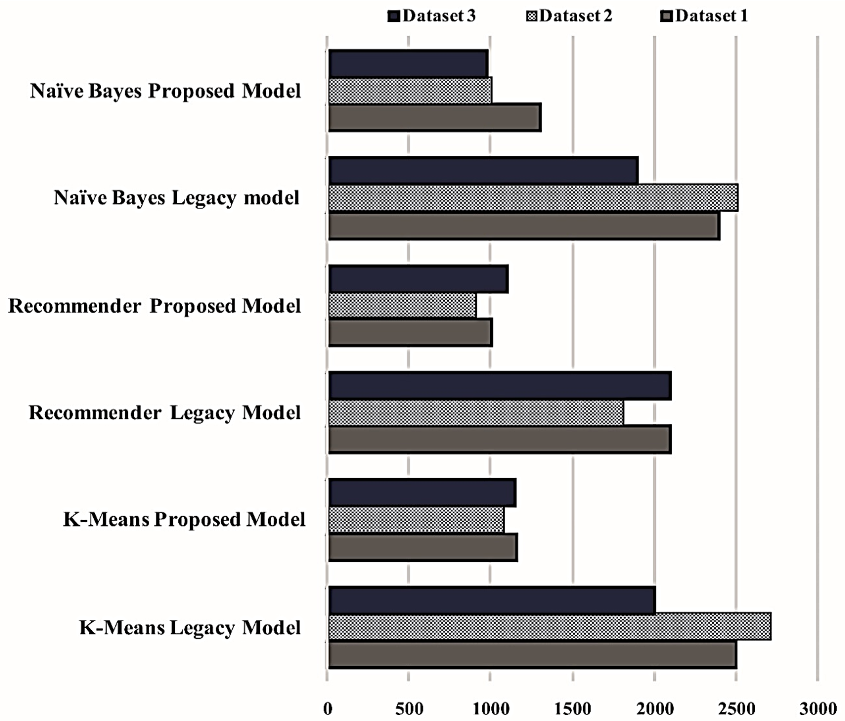
Response time is the total time taken by new stage, submitted stage, analyzing stage and accepted stage. Below, Table 2 defines the response time of K-Means, Naïve Bayes, and recommender algorithms using three different datasets of 9 GB on both models.
Response time defines the quick behavior towards the job instruction submitted to the Name-Node. It is clear from Figure 2 that performance of the proposed model is better than the legacy model in terms of response.

4.2.2. Time Taken (Running Time) by the MapReduce Programming Model

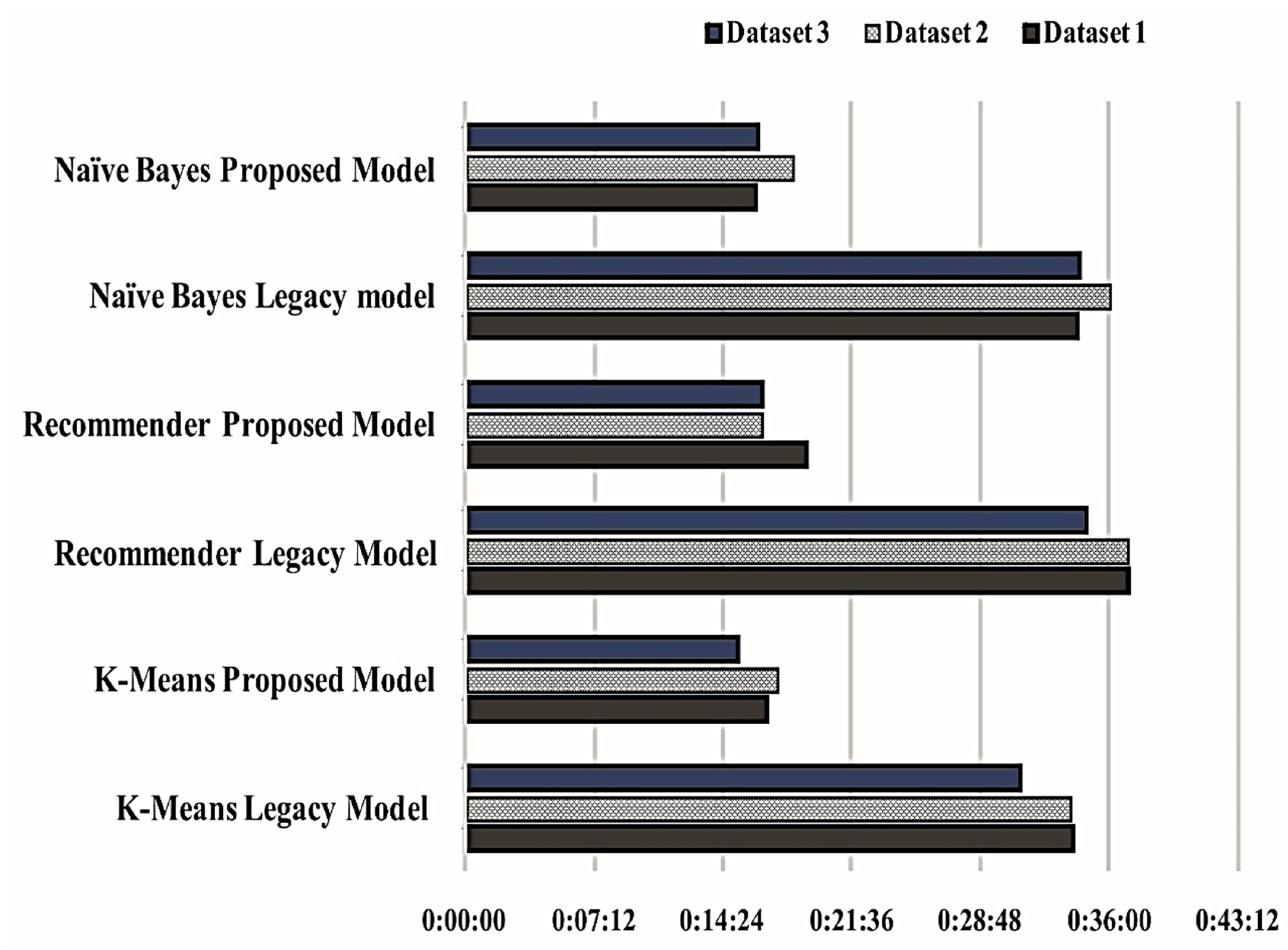
MapReduce programming model has three different phases such as Mapper, Reducer, and Committer. All are processed in a sequence manner. Table 3 shows the time taken by MapReduce programing model (running Stage), to complete three different algorithms using three different data sets on both models.
Figure 3 defines the total time taken by the MapReduce programming model on both models (Proposed and Legacy), while running the K-Means, Recommender, and Naïve Bayes algorithms using three different data sets of 9 GB.

4.2.3. Throughput (Time Taken by the Single Mapper of Map Function)

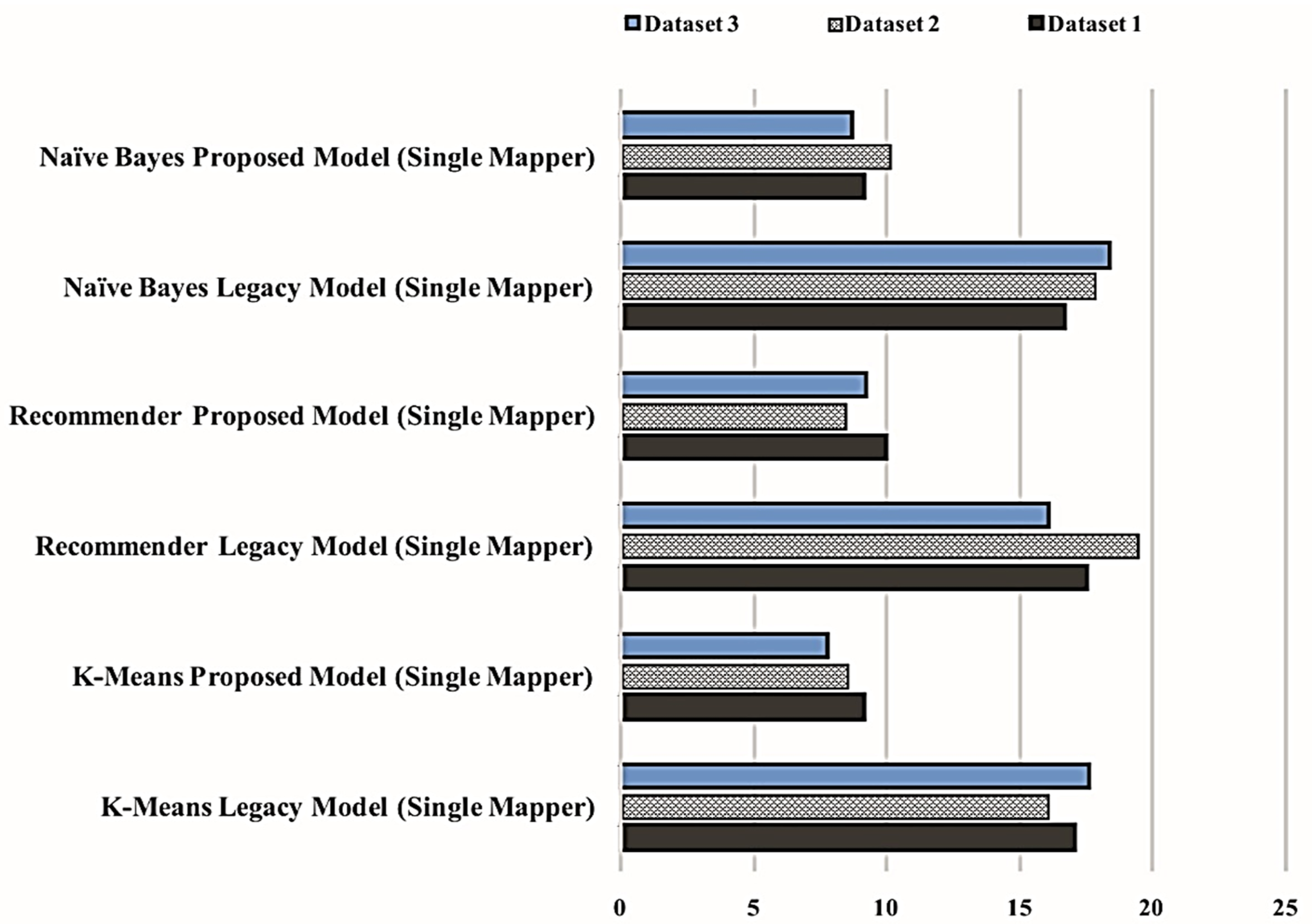
The throughput defines a single unit of work done over a specified time period to evaluate the efficiency of the system [50]. For this, we have calculated the execution time (shown in Table 4) for the single Mapper while executing three different algorithms using three different data sets on both models.
Figure 4 defines throughput measurement, that shows time taken by the single Mapper (single unit of work done) of the MapReduce programming model on both (Proposed and Legacy) models, while running the K-Means, Recommender, and Naïve Bayes algorithms using three different data sets of 9 GB.

5. Discussion

The present paper deals with the performance of the proposed model with respect to the legacy model to measure the difference of response time, running time (time taken by the MapReduce programing model), and throughput. The validation of the proposed model is the process and activities intended to verify its performance as expected, in line with their design objectives. The validation also identifies the potential limitations and assumptions, and assesses their possible impact. The proposed model system configuration, which contains three Name-Node, three Data-Node, and one client node, in which each node has 2 GB of memory and two cores for processing, whereas in the legacy model, memory and CPU size are increased up to 6 GB with four cores. In this way both models have stable 9 GB datasets of three different kinds. In the present work it was expected and assumed that the proposed model should be better response time, running time, and throughput.
Response time in data set 1 of the legacy model and proposed model on three algorithms, i.e., K-means, recommender, and Naïve Bayes, reduced from 2.5 to 1.1, 2.1 to 1.0, 2.4 to 1.3 s, respectively, which is also noticed in Data set 2 and Data set 3. It shows that the proposed model gives a quick response to the job process as compare to the legacy model. MapReduce (Running Time) completion time in data set 1 of the legacy model and proposed model on three algorithms, i.e., K-means, recommender, and Naïve Bayes reduced from 0.33 to 0.16, 0.37 to 0.19, 0.34 to 0.16 h, respectively. When Data set 2 and Data set 3 are run, the same trend of MapReduce completion time is found. It defines that the proposed model completed the Mapper, Reducer, and Committer phase of the MapReduce programming model in less time as compared to the legacy model. Throughput in data set 1 of the legacy model and proposed model on three algorithms, i.e., K-means, recommender, and Naïve Bayes reduced from 17.04 to 9.16, 17.5 to 10, 16.67 to 9.17 s, respectively. A similar pattern is observed in Data set 2 and Data set 3. It defines that the proposed model took less time to complete a single Mapper, which is 128 MB as compared to the Legacy model. The improved performance of the proposed model establishes the hypothesis that our model overcomes the limitation of the resources of the legacy model. The present proposed model configuration performance is given for the first time, so that comparative published/known findings are lacking.
Table 2 defines comparative response time of the both models. It is measured on the basis of total time taken by the four initial stages of the job execution, i.e., the new stage, submitted stage, analyzing stage, and accepted stage. It is evident from Table 2 and Figure 2 that the response time of the three algorithms (K-Means, Naïve Bayes, and recommender) using three different datasets on the proposed model is significantly (P < 0.01) less compared to the legacy model. That denotes the quick response of the proposed model (Infrastructure).
The experiment of the execution time/running stage (time taken by the MapReduce programming model) shown in Table 3 defines MapReduce programing model/running stage (total time taken by the MapReduce programming model) on both models (the proposed and the existing model), respectively. Table 3 clearly indicates that three algorithms (K-Means, Naïve Bayes, and recommender) on three different datasets for proposed model completed their jobs faster than the existing model. In fact, the proposed model took significantly (P < 0.01) less time as compare to the legacy model, as shown in Figure 3.
Table 4 defines the throughputs of the both models using three algorithms (K-Means, Naïve Bayes, and recommender) on three different datasets. According to the definition of the throughput, a single unit of work is done in the specified time period to evaluate the efficiency of the system, so that in this experiment the time taken to complete job by the single mapper of Map function is calculated. It is measured with the help of a data set with chunks the size of a single mapper, which is 128 MB in case of YARN (Yet Another Resource Negotiator). The present study demonstrates that the proposed model is significantly (P < 0.01) efficient compared to the legacy model, as shown in Figure 4.
Therefore, the above findings clearly indicate that the proposed model is better than the legacy model in terms of response time of the system, execution time/running stage (time taken by the MapReduce programing model), and throughput. In addition to this, the proposed model is highly efficient to configure any kind of algorithms and any kind of data of different size simultaneously.

6. Conclusions

Conclusively, the present paper demonstrates that a time-efficient proposed model that shares common HDFS with the integration of three Name-node (having Mahout, R-Hadoop, and Splunk), three Data-node, and one client node, can communicate and share their business demands with all three Name-nodes. Time optimization of our model is done by the performance evaluation of the response time, execution time, and throughput using three different algorithms (K-means clustering, Navies Bayes, and Recommender system) on three different data sets. With the outcome of the definition and the experiments in the present study, it can be concluded that the proposed model is highly efficient compared to the legacy model. In addition to this, by the common HDFS, all the Data-node and Name-node can access any data residing in the HDFS, whether it is processed or used by any other node. Any algorithms on the different types of data can be run efficiently with the help of our present proposed model for Big Data analytics. In the future, the performance of the model can be explored for a bigger number of master nodes as well as data nodes.

Author Contributions

S.V. and B.B.S. analyzed the data and wrote the first draft. K.S. and A.A. validated the results and check the final draft. B.A.P. check the final draft and provide the administration works. All authors have read and agreed to the published version of the manuscript.

Funding

This research was funded by Department of Law, Economics and Human Sciences-Decisions_LAB grant number 2/2020 and the APC was funded by Piano Dipartimento di Eccellenza L.232/2016.

Conflicts of Interest

The authors declare no conflict of interest

References

  1. Garlasu, D.; Sandulescu, V.; Halcu, I.; Neculoiu, G.; Grigoriu, O.; Marinescu, M.; Marinescu, V. A big data implementation based on Grid computing. In Proceedings of the 2013 11th RoEduNet International Conference, Sinaia, Romania, 17–19 January 2013; pp. 1–4. [Google Scholar]
  2. Bryant, R.; Katz, R.H.; Lazowska, E.D. Big-data computing: Creating revolutionary breakthroughs in commerce. Sci. Soc. 2008, 8, 1–15. [Google Scholar]
  3. Gantz, J.; Reinsel, D. Extracting value from chaos. IDC Iview 2011, 1142, 1–12. [Google Scholar]
  4. Chen, L.; Chen, C.P.; Lu, M. A multiple-kernel fuzzy c-means algorithm for image segmentation. IEEE Trans. Syst. Man Cybern. Part B (Cybern.) 2011, 41, 1263–1274. [Google Scholar] [CrossRef] [PubMed]
  5. Gandomi, A.; Haider, M. Beyond the hype: Big data concepts, methods, and analytics. Int. J. Inf. Manag. 2015, 35, 137–144. [Google Scholar] [CrossRef] [Green Version]
  6. Chen, C.P.; Zhang, C.-Y. Data-intensive applications, challenges, techniques and technologies: A survey on Big Data. Inf. Sci. 2014, 275, 314–347. [Google Scholar] [CrossRef]
  7. Rodríguez-Mazahua, L.; Rodríguez-Enríquez, C.-A.; Sánchez-Cervantes, J.L.; Cervantes, J.; García-Alcaraz, J.L.; Alor-Hernández, G. A general perspective of Big Data: Applications, tools, challenges and trends. J. Supercomput. 2016, 72, 3073–3113. [Google Scholar] [CrossRef]
  8. Hashem, I.A.T.; Yaqoob, I.; Anuar, N.B.; Mokhtar, S.; Gani, A.; Khan, S.U. The rise of “big data” on cloud computing: Review and open research issues. Inf. Syst. 2015, 47, 98–115. [Google Scholar] [CrossRef]
  9. Bhati, J.P.; Tomar, D.; Vats, S. Examining Big Data Management Techniques for Cloud-Based IoT Systems. In Examining Cloud Computing Technologies Through the Internet of Things; IGI Global: Hershey, PA, USA, 2018; pp. 164–191. [Google Scholar]
  10. Vats, S.; Sagar, B. Data Lake: A plausible Big Data science for business intelligence. In Proceedings of the 2nd International Conference on Communication and Computing Systems (ICCCS 2018), Gurgaon, India, 1–2 December 2018; p. 442. [Google Scholar]
  11. Agarwal, R.; Singh, S.; Vats, S. Review of Parallel Apriori Algorithm on MapReduce Framework for Performance Enhancement. In Big Data Analytics; Springer: Dordrecht, The Netherlands, 2018; pp. 403–411. [Google Scholar]
  12. Arias, J.; Gamez, J.A.; Puerta, J.M. Learning distributed discrete Bayesian network classifiers under MapReduce with Apache spark. Knowl. Based Syst. 2017, 117, 16–26. [Google Scholar] [CrossRef]
  13. Semberecki, P.; Maciejewski, H. Distributed classification of text documents on Apache Spark platform. In Proceedings of the International Conference on Artificial Intelligence and Soft Computing, Zakapane, Poland, 12–16 June 2016; pp. 621–630. [Google Scholar]
  14. Shen, P.; Wang, H.; Meng, Z.; Yang, Z.; Zhi, Z.; Jin, R.; Yang, A. An improved parallel Bayesian text classification algorithm. Rev. Comput. Eng. Stud. 2016, 3, 6–10. [Google Scholar]
  15. Prabhat, A.; Khullar, V. Sentiment classification on big data using Naïve Bayes and logistic regression. In Proceedings of the 2017 International Conference on Computer Communication and Informatics (ICCCI), Coimbatore, India, 5–7 January 2017; pp. 1–5. [Google Scholar]
  16. Kotwal, A.; Fulari, P.; Jadhav, D.; Kad, R. Improvement in sentiment analysis of twitter data using hadoop. In Proceedings of the International Conference on “Computing for Sustainable Global Development”, New Delhi, India, 16–18 March 2016. [Google Scholar]
  17. Sheela, L.J. A review of sentiment analysis in twitter data using Hadoop. Int. J. Database Theory Appl. 2016, 9, 77–86. [Google Scholar] [CrossRef]
  18. Hou, X. An Improved K-means Clustering Algorithm Based on Hadoop Platform. In Proceedings of the International Conference on Cyber Security Intelligence and Analytics, Shenyang, China, 21–22 February 2019; pp. 1101–1109. [Google Scholar]
  19. Ansari, Z.; Afzal, A.; Sardar, T.H. Data Categorization Using Hadoop MapReduce-Based Parallel K-Means Clustering. J. Inst. Eng. India Ser. B 2019, 100, 95–103. [Google Scholar] [CrossRef]
  20. Shaikh, T.A.; Shafeeque, U.B.; Ahamad, M. An Intelligent Distributed K-means Algorithm over Cloudera/Hadoop. Int. J. Educ. Manag. Eng. 2018, 8, 61. [Google Scholar] [CrossRef]
  21. Yang, M.; Mei, H.; Huang, D. An effective detection of satellite image via K-means clustering on Hadoop system. Int. J. Innov. Comput. Inf. Control 2017, 13, 1037–1046. [Google Scholar]
  22. Wang, Y.; Wang, M.; Xu, W. A sentiment-enhanced hybrid recommender system for movie recommendation: A big data analytics framework. Wirel. Commun. Mob. Comput. 2018, 2018, 8263740. [Google Scholar] [CrossRef] [Green Version]
  23. Zhang, H.; Huang, T.; Lv, Z.; Liu, S.; Zhou, Z. MCRS: A course recommendation system for MOOCs. Multimed. Tools Appl. 2018, 77, 7051–7069. [Google Scholar] [CrossRef]
  24. McClay, W. A Magnetoencephalographic/encephalographic (MEG/EEG) brain-computer interface driver for interactive iOS mobile videogame applications utilizing the Hadoop Ecosystem, MongoDB, and Cassandra NoSQL databases. Diseases 2018, 6, 89. [Google Scholar] [CrossRef] [Green Version]
  25. Bharti, R.; Gupta, D. Recommending top N movies using content-based filtering and collaborative filtering with hadoop and hive framework. In Recent Developments in Machine Learning and Data Analytics; Springer: Dordrecht, The Netherlands, 2019; pp. 109–118. [Google Scholar]
  26. Contratres, F.G.; Alves-Souza, S.N.; Filgueiras, L.V.L.; DeSouza, L.S. Sentiment analysis of social network data for cold-start relief in recommender systems. In Proceedings of the World Conference on Information Systems and Technologies, Galicia, Spain, 16–19 April 2018; pp. 122–132. [Google Scholar]
  27. Sherman, B.T.; Lempicki, R.A. Systematic and integrative analysis of large gene lists using DAVID bioinformatics resources. Nat. Protoc. 2009, 4, 44. [Google Scholar]
  28. Lavrac, N.; Keravnou, E.; Zupan, B. Intelligent data analysis in medicine. Encycl. Comput. Sci. Technol. 2000, 42, 113–157. [Google Scholar]
  29. Sharma, I.; Tiwari, R.; Rana, H.S.; Anand, A. Analysis of mahout big data clustering algorithms. In Intelligent Communication, Control and Devices; Springer: Dordrecht, The Netherlands, 2018; pp. 999–1008. [Google Scholar]
  30. Almeida, F.; Calistru, C. The main challenges and issues of big data management. Int. J. Res. Stud. Comput. 2013, 2, 11–20. [Google Scholar] [CrossRef]
  31. Ghemawat, S.; Gobioff, H.; Leung, S.-T. The Google file system. In Proceedings of the nineteenth ACM symposium on Operating systems principles, Bolton Landing, NY, USA, 19–22 October 2003; pp. 29–43. [Google Scholar]
  32. Dean, J.; Ghemawat, S. MapReduce: Simplified data processing on large clusters. Commun. ACM 2008, 51, 107–113. [Google Scholar] [CrossRef]
  33. Apache Hadoop (2012). Available online: http://hadoop.apache.org/ (accessed on 21 June 2020).
  34. Shvachko, K.; Kuang, H.; Radia, S.; Chansler, R. The hadoop distributed file system. In Proceedings of the 2010 IEEE 26th Symposium on Mass Storage Systems and Technologies (MSST), Incline Village, NV, USA, 3–7 May 2010; pp. 1–10. [Google Scholar]
  35. Bhandarkar, M. MapReduce programming with apache Hadoop. In Proceedings of the 2010 IEEE International Symposium on Parallel & Distributed Processing (IPDPS), Atlanta, GA, USA, 19–23 April 2010; p. 1. [Google Scholar]
  36. Apache Mahout (2019). Available online: https://mahout.apache.org/ (accessed on 21 June 2020).
  37. Apache Hbase (2019). Available online: http://hbase.apache.org/ (accessed on 21 June 2020).
  38. Apache Hive (2019). Available online: http://hive.apache.org/ (accessed on 21 June 2020).
  39. Esteves, R.M.; Pais, R.; Rong, C. K-means clustering in the cloud—A Mahout test. In Proceedings of the 2011 IEEE Workshops of International Conference on Advanced Information Networking and Applications, Biopolis, Singapore, 22–25 March 2011; pp. 514–519. [Google Scholar]
  40. Rong, C. Using Mahout for clustering Wikipedia’s latest articles: A comparison between k-means and fuzzy c-means in the cloud. In Proceedings of the 2011 IEEE Third International Conference on Cloud Computing Technology and Science, Washington, DC, USA, 5–10 July 2011; pp. 565–569. [Google Scholar]
  41. Ericson, K.; Pallickara, S. On the performance of high dimensional data clustering and classification algorithms. Future Gener. Comput. Syst. 2013, 29, 1024–1034. [Google Scholar] [CrossRef] [Green Version]
  42. Chakraborty, T.; Jajodia, S.; Katz, J.; Picariello, A.; Sperli, G.; Subrahmanian, V. FORGE: A fake online repository generation engine for cyber deception. In IEEE Transactions on Dependable and Secure Computing; IEEE: Piscataway, NJ, USA, 2019. [Google Scholar] [CrossRef]
  43. Mercorio, F.; Mezzanzanica, M.; Moscato, V.; Picariello, A.; Sperli, G. DICO: A graph-db framework for community detection on big scholarly data. In IEEE Transactions on Emerging Topics in Computing; IEEE: Piscataway, NJ, USA, 2019. [Google Scholar] [CrossRef]
  44. Moscato, V.; Picariello, A.; Sperlí, G. Community detection based on game theory. Eng. Appl. Artif. Intell. 2019, 85, 773–782. [Google Scholar] [CrossRef]
  45. Agarwal, R.; Singh, S.; Vats, S. Implementation of an improved algorithm for frequent itemset mining using Hadoop. In Proceedings of the 2016 International Conference on Computing, Communication and Automation (ICCCA), Greater Noida, India, 29–30 April 2016; pp. 13–18. [Google Scholar]
  46. Vats, S.; Sagar, B. Performance evaluation of K-means clustering on Hadoop infrastructure. J. Discret. Math. Sci. Cryptogr. 2019, 22, 1349–1363. [Google Scholar] [CrossRef]
  47. News Group. Available online: https://www.kaggle.com/crawford/20-newsgroups (accessed on 21 June 2020).
  48. Netflix. Available online: https://www.kaggle.com/laowingkin/netflix-movie-recommendation/data (accessed on 21 June 2020).
  49. Sms-spam-classification. Available online: https://www.kaggle.com/jeandsantos/sms-spam-classification/activity (accessed on 21 June 2020).
  50. Landset, S.; Khoshgoftaar, T.M.; Richter, A.N.; Hasanin, T. A survey of open source tools for machine learning with big data in the Hadoop ecosystem. J. Big Data 2015, 2, 24. [Google Scholar] [CrossRef] [Green Version]
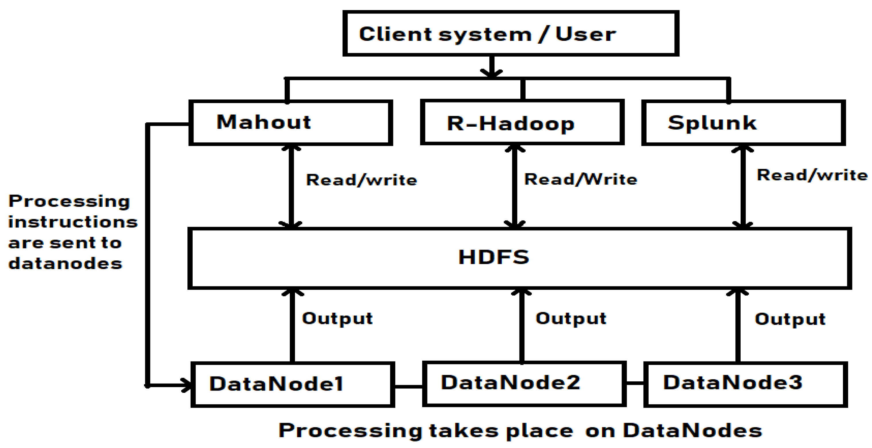
Figure 1. Block diagram of the proposed model.
Symmetry 12 01274 g001
Figure 2. Response time of both models.
Symmetry 12 01274 g002
Figure 3. Total time taken by the MapReduce Programming Model.
Symmetry 12 01274 g003
Figure 4. Throughput measurement of the Proposed and Legacy model.
Symmetry 12 01274 g004
Table 1. 10Vs of Big Data.
VolumeData at rest
VelocityData in motion
VarietyData in many form
VeracityData in doubt
VariabilityData in inconsistency speed
ValidityData for accuracy
VolatilityData is unstable or changeable
VulnerabilityData for privacy
VisualizationData for imagination
ValueData for benefits
Table 2. Response time (in millisecond).
Algorithms with EnvironmentDataset 1Dataset 2Dataset 3
K-Means Legacy Model* 2500 ± 2.59* 2700 ± 2.82* 2000 ± 2.72
K-Means Proposed Model* 1155 ± 3.57* 1075 ± 1.86* 1150 ± 1.41
Recommender Legacy Model* 2100 ± 1.41* 1800 ± 0.94* 2100 ± 1.41
Recommender Proposed Model* 1009 ± 1.86* 900 ± 2.82* 1100 ± 2.82
Naïve Bayes Legacy model* 2400 ± 2.35* 2500 ± 1.88* 1900 ± 1.41
Naïve Bayes Proposed Model* 1300 ± 1.41* 1000 ± 0.94* 975 ± 1.41
Significant, when student’s t-test is applied in between response time of legacy and proposed model- * (P < 0.01). Values are given as mean ± SE.
Table 3. Total time taken by the MapReduce Programming Model.
Algorithms with EnvironmentDataset 1Dataset 2Dataset 3
K-Means Legacy Model* 0:33:55 ± 0.28* 0:33:46 ± 0.02* 0:31:00 ± 0.02
K-Means Proposed Model* 0:16:50 ± 0.24* 0:17:28 ± 0.04* 0:15:16 ± 0.02
Recommender Legacy Model* 0:37:00 ± 0.03* 0:37:01 ± 0.01* 0:34:46 ± 0.02
Recommender Proposed Model* 0:19:01 ± 0.01* 0:16:34 ± 0.02* 0:16:37 ± 0.03
Naïve Bayes Legacy model* 0:34:13 ± 0.01* 0:36:00 ± 0.01* 0:34:17 ± 0.03
Naïve Bayes Proposed Model* 0:16:15 ± 0.02* 0:18:15 ± 0.01* 0:16:20 ± 0.03
Significant when student’s t-test is applied in between response time of legacy and proposed model—* (P < 0.01). Values are given as mean ± SE.
Table 4. Execution time (for single Mapper) in seconds.
Algorithms with EnvironmentDataset 1Dataset 2Dataset 3
K-Means Legacy Model (Single Mapper)* 17.04 ± 0.01* 16.02 ± 0.01* 17.62 ± 0.01
K-Means Proposed Model (Single Mapper)* 9.16 ± 0.01* 8.51 ± 0.01* 7.75 ± 0.02
Recommender Legacy Model (Single Mapper)* 17.5 ± 0.18* 19.4 ± 0.18* 16.06 ± 0.02
Recommender Proposed Model (Single Mapper)* 10.0 ± 0.47* 8.45 ± 0.02* 9.2 ± 0.09
Naïve Bayes Legacy model (Single Mapper)* 16.67 ± 0.07* 17.78 ± 0.03* 18.34 ± 0.01
Naïve Bayes Proposed Model (Single Mapper)* 9.17 ± 0.03* 10.1 ± 0.13* 8.67 ± 0.03
Significant when student’s t-test is applied in between response time of legacy and proposed model—* (P < 0.01). Values are given as mean ± SE.