Explicit Properties of q-Cosine and q-Sine Euler Polynomials Containing Symmetric Structures

Abstract

In this paper, we introduce q-cosine and q-sine Euler polynomials and determine identities for these polynomials. From these polynomials, we obtain some special properties using a power series of q-trigonometric functions, properties of q-exponential functions, and q-analogues of the binomial theorem. We investigate the approximate roots of q-cosine Euler polynomials that help us understand these polynomials. Moreover, we display the approximate roots movements of q-cosine Euler polynomials in a complex plane using the Newton method.

1. Introduction

In 1990, Jackson who published influential papers on the subject introduced the q-number and its notation stems, see [1]. Floreanini and Vinet found that some properties of q-orthogonal polynomials are connected to the q-oscillator algebra in [1,2,3,4]. We begin by introducing several definitions related to q-numbers used in this paper, see [3,5,6,7,8].

Throughout this paper, the symbols, $\mathbb{N},\mathbb{Z},\mathbb{R}$ and $\mathbb{C}$ denotes the set of natural numbers, the set of integers, the set of real numbers and the set of complex numbers, respectively.

For $a\in \mathbb{C}$, $n\in \mathbb{N}$ and $\left|q\right|<1$, the q-shifted factorial is defined by

$${(a;q)}_0=1,{(a;q)}_n={\displaystyle \prod _{j=0}^{n-1}}(1-q^{j}a),{(a;q)}_{\infty }={\displaystyle \prod _{j=0}^{\infty }}(1-q^{j}a).$$

(1)

It is well known that

$${(a;q)}_n={\displaystyle \sum _{k=0}^n}{\left[\begin{array}{l}n\\ k\end{array}\right]}_q{q}^{(1/2)k(k-1)}{(-1)}^k{a}^k.$$

(2)

Let $x,q\in \mathbb{R}$ with $q\ne 1$. The number

$${\left[x\right]}_q=\frac{1-q^x}{1-q}$$

(3)

is called q-number. We note that ${lim}_{q\to 1}{\left[x\right]}_q=x$. In particular, for $k\in \mathbb{Z}$, ${\left[k\right]}_q$ is a q-integer.

After the appearance of q-numbers, many mathematicians have studied topics such as q-differential equations, q-series, and q-trigonometric functions. Of course, mathematicians also constructed and researched q-Gaussian binomial coefficients, see [2,3,4,7,8,9,10,11].

Definition 1.

For $r\le m$ and $m,r\in \mathbb{N}$, the q-Gaussian binomial coefficients are defined by

$${\left[\begin{array}{l}m\\ r\end{array}\right]}_q=\frac{{(q;q)}_m}{{(q;q)}_{m-r}{(q;q)}_r}.$$

(4)

For $r=0$, we note that ${\left[\begin{array}{l}m\\ 0\end{array}\right]}_q=0$ with $0\le r\le m$, and also, we note that ${\left[n\right]}_q!={\left[n\right]}_q\cdots {\left[2\right]}_q{\left[1\right]}_q$ and ${\left[0\right]}_q$!=1.

Definition 2.

Let $0<\left|q\right|<1$ and $\left|z\right|<\frac{1}{|1-q|}$. Then, the q-exponential function is defined by

$$e_q\left(z\right)={\displaystyle \sum _{n=0}^{\infty }}\frac{z^n}{{\left[n\right]}_q!}={\displaystyle \prod _{k=0}^{\infty }}\frac{1}{(1-(1-q)q^{k}z)}.$$

(5)

For $0<q<1$ and $\left|z\right|<\frac{2}{1-q}$, the other form of q-exponential function can be defined as

$$E_q\left(z\right)=e_{q^{-1}}\left(z\right)={\displaystyle \sum _{n=0}^{\infty }}{q}^{\left(\genfrac{}{}{0pt}{}{n}{2}\right)}\frac{z^n}{{\left[n\right]}_q!}={\displaystyle \prod _{k=0}^{\infty }}(1+(1-q)q^{k}z).$$

(6)

We note that ${lim}_{q\to 1}{e}_q\left(z\right)=e^z$. Exponential function is expanded to the power series expressions of the two q-exponential functions by combining with q-numbers. Also, q-derivatives and q-integrals were extensively studied by many mathematicians, see [1,5,12]. Following the determination of the limit formulas for q-exponential functions taken from Rawlings [10], several other interesting q-series expansions were presented in the classical book by Andrews [5].

Theorem 1.

From Definition 2, we note that

$$\begin{array}{ll}\left(i\right)& e_q\left(x\right)e_q\left(y\right)=e_q(x+y),ifyx=qxy.\\ \left(ii\right)& e_q\left(x\right)E_q(-x)=1.\end{array}$$

(7)

The proof of Theorem 1 and more properties of q-exponential functions can be found in [2,13].

Definition 3.

For real variable function f where $x\ne 0$, the q-derivative operator is defined as

$$D_{q}f\left(x\right)=\frac{f\left(x\right)-f\left(qx\right)}{(1-q)x}.$$

(8)

We note that $D_{q}f\left(0\right)=f^{\prime }\left(0\right)$. It is possible to prove that f is differentiable at 0 and it is clear that $D_q{x}^n={\left[n\right]}_q{x}^{n-1}$.

In 2002, Kac and Pokman published a book about quantum calculus including q-derivatives and q-analogue of ${(x-a)}^n$ and q-trigonometric functions, see [14].

Definition 4.

Let n be a nonnegative integer. The q-analogues of subtraction and addition are defined by

$$\begin{array}{ll}\left(i\right) {(x\ominus a)}_q^n& =\{\begin{array}{ll}1\hfill & ifn=0\hfill \\ (x-a)(x-qa)\cdots (x-q^{n-1}a)\hfill & ifn\ge 1\hfill \end{array}\\ & ={\displaystyle \sum _{k=0}^n}{\left[\begin{array}{l}n\\ k\end{array}\right]}_q\frac{{(-1;q)}_k{(-1;q)}_{n-k}}{2^n}{x}^k{a}^{n-k},\\ \left(ii\right) {(x\oplus a)}_q^n& =\left\{\begin{array}{ll}1\hfill & ifn=0\hfill \\ (x+a)(x+qa)\cdots (x+q^{n-1}a)\hfill & ifn\ge 1\hfill \end{array}\right.\\ & ={\displaystyle \sum _{k=0}^n}{\left[\begin{array}{l}n\\ k\end{array}\right]}_q\frac{{(-1;q)}_k{(-1;q)}_{n-k}}{2^n}{x}^k{(-a)}^{n-k},\\ respectively.& \end{array}$$

(9)

Definition 5.

Let $x\in \mathbb{R}$ and $i=\sqrt{-1}$. Then, the q-trigonometric functions are defined by

$$\begin{array}{ll}{\mathit{sin}}_q\left(x\right)& =\frac{e_q\left(ix\right)-e_q(-ix)}{2i},{\mathit{sin}}_q\left(x\right)=\frac{E_q\left(ix\right)-E_q(-ix)}{2i}\\ {\mathit{cos}}_q\left(x\right)& =\frac{e_q\left(ix\right)+e_q(-ix)}{2},{\mathit{cos}}_q\left(x\right)=\frac{E_q\left(ix\right)+E_q(-ix)}{2},\end{array}$$

(10)

where ${\mathit{sin}}_q\left(x\right)={\mathit{sin}}_{q^{-1}}\left(x\right),{\mathit{cos}}_q\left(x\right)={\mathit{cos}}_{q^{-1}}\left(x\right)$.

Theorem 2.

Using Theorem 1 $\left(ii\right)$ and applying the chain rule, we have

$$\begin{array}{ll}\left(i\right)& {\mathit{cos}}_q\left(x\right){\mathit{cos}}_q\left(x\right)+{\mathit{sin}}_q\left(x\right){\mathit{sin}}_q\left(x\right)=1.\\ \left(ii\right)& \left\{\begin{array}{ll}{D}_q{\mathit{sin}}_q\left(x\right)={\mathit{cos}}_q\left(x\right),\hfill & D_q{\mathit{sin}}_q\left(x\right)={\mathit{cos}}_q\left(x\right),\hfill \\ D_q{\mathit{cos}}_q\left(x\right)=-{\mathit{sin}}_q\left(x\right),\hfill & D_q{\mathit{cos}}_q\left(x\right)=-{\mathit{sin}}_q\left(x\right).\hfill \end{array}\right.\end{array}$$

(11)

Moreover, we note Theorem 2 $\left(i\right)$ is the q-analogue of the identity ${\mathit{sin}}^{2}x+{\mathit{cos}}^{2}x=1$, see [3,4,7].

In 2004, Gasper and Rahman introduced a comprehensive account of the basic q-hypergeometric series, see [4]. During the last three decades, one of the bridges between science and applied mathematics has been q-calculus, see [10]. Based on the above concepts, many mathematicians explored various fields of mathematics including q-differential equations, q-series, q-hypergeometric functions, and q-gamma and q-beta functions. Moreover, various discrete distributions combining q-numbers can be found in [2]. Therefore, q-calculus plays an important role in many different areas of mathematics.

Many researchers who studied the Bernoulli, Euler, and Genocchi polynomials in various fields realized the important role of q-calculus in mathematics. For a long time, the topics of Bernoulli, Euler, and Genocchi polynomials have been extensively researched in many mathematical applications including analytical number theory, combinatorial analysis, p-adic analytic number theory, and other fields. Therefore, many mathematicians have started researching Bernoulli, Euler, and Genocchi polynomials combining q-numbers, see [9,13,15,16,17,18,19,20,21].

The following diagram briefly explains the relation between the various types of degenerate Euler polynomials, Euler polynomials, and q-Euler polynomials. The polynomials in the first row are researched by Calitz [21], Kim and Ryoo [16], respectively. The study of the second row of the diagram has brought about beneficial results in combinatorics and number theory. In particular, the cosine and sine Euler polynomials in the second row of the diagram contain a motive in this paper. This is because we hold several questions regarding what is a definition form of q-cosine and q-sine Euler polynomials and what is different properties between the q-cosine, q-sine Euler polynomials and the cosine, sine Euler polynomials.

The main subject of this paper is to construct q-cosine and q-sine Euler polynomials using Definitions 4 and 5. Also, we derive identities and properties for these polynomials in the third row of the diagram.

The definition of q-Euler polynomials of the third row are as follows.

Definition 6.

The q-Euler numbers and polynomials are defined respectively as see [19]

$${\displaystyle \sum _{n=0}^{\infty }}{E}_{n,q}\frac{t^n}{n!}=\frac{2}{e_q\left(t\right)+1},{\displaystyle \sum _{n=0}^{\infty }}{E}_{n,q}\left(z\right)\frac{t^n}{n!}=\frac{2}{e_q\left(t\right)+1}{e}_q\left(tz\right),$$

(12)

.

Recently, Kim and Ryoo introduced the basic concepts of cosine and sine Euler polynomials. In [16], the definitions and representative properties of cosine and sine Euler polynomials are as follows.

Definition 7.

The cosine Euler polynomials $E_n^{\left(C\right)}(x,y)$ and the sine Euler polynomials $E_n^{\left(S\right)}(x,y)$ are defined by means of the generating functions

$${\displaystyle \sum _{n=0}^{\infty }}{E}_n^{\left(C\right)}(x,y)\frac{t^n}{n!}=\frac{2}{e^t+1}{e}^{tx}\mathit{cos}\left(ty\right),{\displaystyle \sum _{n=0}^{\infty }}{E}_n^{\left(S\right)}(x,y)\frac{t^n}{n!}=\frac{2}{e^t+1}{e}^{tx}\mathit{sin}\left(ty\right).$$

(13)

In this paper, we denote that $E_n^{\left(C\right)}(x,y)={}_C{\mathcal{E}}_n(x,y)$ and $E_n^{\left(S\right)}(x,y)={}_S{\mathcal{E}}_n(x,y)$.

Theorem 3.

For $n\ge 1$, we have

$$\begin{array}{ll}\left(i\right)& E_n^{\left(C\right)}(x+1,y)-E_n^{\left(C\right)}(x,y)=2C_n(x,y),\\ \left(ii\right)& E_n^{\left(S\right)}(x+1,y)-E_n^{\left(S\right)}(x,y)=2S_n(x,y).\end{array}$$

(14)

Based on [16], which contains Definition 7 and Theorem 3, many researchers found various expanded numbers and polynomials and their identities, see [15,20].

The main goal of this paper is to find various properties of q-cosine and q-sine Euler polynomials such as addition theorem, partial q-derivative, basic symmetric properties so on. In Section 2, we construct q-cosine and q-sine Euler polynomials. Then, using q-calculus, we identify basic properties of these polynomials. Section 3 presents an investigation of the special properties of q-cosine and q-sine Euler polynomials such as the identity of q-sine Euler polynomials using q-analogues of subtraction and addition. This is based on the properties of q-trigonometric and q-exponential functions. Moreover, we derive relationships between q-cosine and q-sine Euler polynomials and q-cosine and q-sine Bernoulli polynomials. In Section 4, we display the structure of approximate roots for q-cosine and q-sine Euler polynomials and find properties of these polynomials. We present some figures of the approximate roots of these polynomials in a complex plane using Newton’s method.

2. Some Basic Properties of q-cosine and q-sine Euler Polynomials

In this section, we construct the q-cosine and q-sine Euler polynomials by using Theorem 4. From the generating functions of these polynomials, we obtain some basic properties and identities. Moreover, we derive symmetric properties and partial q-derivatives for q-cosine and q-sine Euler polynomials.

Definition 8.

The generating functions of q-cosine Euler polynomials and q-sine Euler polynomials are correspondingly defined by

$$\begin{gathered} {\displaystyle \sum _{n=0}^{\infty }}{}_C{\mathcal{E}}_{n,q}(x,y)\frac{t^n}{{\left[n\right]}_q!}=\frac{2}{e_q\left(t\right)+1}{e}_q\left(tx\right)CO{S}_q\left(ty\right) \\ and \\ {\displaystyle \sum _{n=0}^{\infty }}{}_S{\mathcal{E}}_{n,q}(x,y)\frac{t^n}{{\left[n\right]}_q!}=\frac{2}{e_q\left(t\right)+1}{e}_q\left(tx\right)SI{N}_q\left(ty\right). \end{gathered}$$

(15)

From Definition 8, q-sine Euler polynomials can be confirmed as the following:

$$\begin{array}{lll}{}_S{\mathcal{E}}_{0,q}(x,y)& =& 0,\\ {}_S{\mathcal{E}}_{1,q}(x,y)& =& -\frac{y}{1+q},\\ {}_S{\mathcal{E}}_{2,q}(x,y)& =& -\frac{(1+q+q^2-2x)y}{2(1+q+q^2)},\\ {}_S{\mathcal{E}}_{3,q}(x,y)& =& -\frac{y(1+2x+2qx-4x^2+q^2(1+2x)+q^5(-1+4y^2)+q^3(-1+2x+4y^2))}{4(1+q)(1+q^2)},\\ \cdots .\end{array}$$

We will introduce the certain form of q-cosine Euler polynomials in Section 4. The motivation to derive the definition of q-cosine Euler polynomials and q-sine Euler polynomials can be found in Theorem 4.

Theorem 4.

For $x,y\in \mathbb{R}$ and $i=\sqrt{-1}$, we have

$$\begin{array}{ll}\left(i\right)& {\displaystyle \sum _{n=0}^{\infty }}\left(\frac{{\mathcal{E}}_{n,q}\left({(x\oplus iy)}_q\right)+{\mathcal{E}}_{n,q}\left({(x\ominus iy)}_q\right)}{2}\right)\frac{t^n}{{\left[n\right]}_q!}=\frac{2}{e_q\left(t\right)+1}{e}_q\left(tx\right)CO{S}_q\left(ty\right),\\ \left(ii\right)& {\displaystyle \sum _{n=0}^{\infty }}\left(\frac{{\mathcal{E}}_{n,q}\left({(x\oplus iy)}_q\right)-{\mathcal{E}}_{n,q}\left({(x\ominus iy)}_q\right)}{2i}\right)\frac{t^n}{{\left[n\right]}_q!}=\frac{2}{e_q\left(t\right)+1}{e}_q\left(tx\right)SI{N}_q\left(ty\right).\end{array}$$

(16)

Proof. 

$\left(i\right)$ We defined the generating function of q-Euler polynomials in Definition 6. Let us substitute ${(x\oplus iy)}_q$ instead of z in the q-Euler polynomials. By using a property of q-analogues of the sine and cosine functions and by using Definition 1, we can find

$$\begin{array}{lll}{\displaystyle \sum _{n=0}^{\infty }}{\mathcal{E}}_{n,q}\left({(x\oplus iy)}_q\right)\frac{t^n}{{\left[n\right]}_q!}& =& \frac{2}{e_q\left(t\right)+1}{\displaystyle \sum _{n=0}^{\infty }}{(x\oplus iy)}_q^n\frac{t^n}{{\left[n\right]}_q!}\\ & =& \frac{2}{e_q\left(t\right)+1}{\displaystyle \sum _{n=0}^{\infty }}\left({\displaystyle \sum _{k=0}^n}{\left[\begin{array}{l}n\\ k\end{array}\right]}_q{q}^{\left(\genfrac{}{}{0pt}{}{n-k}{2}\right)}{x}^k{\left(iy\right)}^{n-k}\right)\frac{t^n}{{\left[n\right]}_q!}\\ & =& \frac{2}{e_q\left(t\right)+1}{e}_q\left(tx\right)E_q\left(ity\right)\\ & =& \frac{2}{e_q\left(t\right)+1}{e}_q\left(tx\right)\left(CO{S}_q\left(ty\right)+iSI{N}_q\left(ty\right)\right).\end{array}$$

(17)

By using a similar method as when finding Equation (17), we can also obtain

$$\begin{array}{lll}{\displaystyle \sum _{n=0}^{\infty }}{\mathcal{E}}_{n,q}\left({(x\ominus iy)}_q\right)\frac{t^n}{{\left[n\right]}_q!}& =& \frac{2}{e_q\left(t\right)+1}{e}_q\left(tx\right)E_q(-ity)\\ & =& \frac{2}{e_q\left(t\right)+1}{e}_q\left(tx\right)\left(CO{S}_q\left(ty\right)-iSI{N}_q\left(ty\right)\right).\end{array}$$

(18)

$\left(ii\right)$ We can prove Theorem 4 $\left(ii\right)$ through Equations (17) and (18). ☐

Remark 1.

From the Theorem 4 and Definition 8, the following holds

$$\begin{array}{ll}\left(i\right)& {}_C{\mathcal{E}}_{n,q}(x,y)=\frac{{\mathcal{E}}_{n,q}\left({(x\oplus iy)}_q\right)+{\mathcal{E}}_{n,q}\left({(x\ominus iy)}_q\right)}{2}\\ \left(ii\right)& {}_S{\mathcal{E}}_{n,q}(x,y)=\frac{{\mathcal{E}}_{n,q}\left({(x\oplus iy)}_q\right)-{\mathcal{E}}_{n,q}\left({(x\ominus iy)}_q\right)}{2i}.\end{array}$$

(19)

In [15], $C_{n,q}(x,y)$ and $S_{n,q}(x,y)$ are defined as follows:

$$\begin{array}{ll}\left(i\right)& {\displaystyle \sum _{n=0}^{\infty }}{C}_{n,q}(x,y)\frac{t^n}{{\left[n\right]}_q!}=e_q\left(tx\right)CO{S}_q\left(ty\right),\\ \left(ii\right)& {\displaystyle \sum _{n=0}^{\infty }}{S}_{n,q}(x,y)\frac{t^n}{{\left[n\right]}_q!}=e_q\left(tx\right)SI{N}_q\left(ty\right).\end{array}$$

(20)

Theorem 5.

For any real numbers $x,y$, we have

$$\begin{array}{ll}\left(i\right)& {}_C{\mathcal{E}}_{n,q}(x,y)={\displaystyle \sum _{k=0}^n}{\left[\begin{array}{l}n\\ k\end{array}\right]}_q{E}_{k,q}{C}_{n-k,q}(x,y),\\ \left(ii\right)& {}_S{\mathcal{E}}_{n,q}(x,y)={\displaystyle \sum _{k=0}^n}{\left[\begin{array}{l}n\\ k\end{array}\right]}_q{E}_{k,q}{S}_{n-k,q}(x,y),\end{array}$$

(21)

where $E_{n,q}$ is the q-Euler numbers.

Proof. 

$\left(i\right)$ From the generating function of q-cosine Euler polynomials, we can find a relation between the q-Euler numbers and $C_{n,q}(x,y)$ as follows.

$$\begin{array}{lll}{\displaystyle \sum _{n=0}^{\infty }}{}_C{\mathcal{E}}_{n,q}(x,y)\frac{t^n}{{\left[n\right]}_q!}& =& {\displaystyle \sum _{n=0}^{\infty }}{}_C{E}_{n,q}\frac{t^n}{{\left[n\right]}_q!}{\displaystyle \sum _{n=0}^{\infty }}{C}_{n,q}(x,y)\frac{t^n}{{\left[n\right]}_q!}\\ & =& {\displaystyle \sum _{n=0}^{\infty }}\left({\displaystyle \sum _{k=0}^n}{\left[\begin{array}{l}n\\ k\end{array}\right]}_q{E}_{k,q}{C}_{n-k,q}(x,y)\right)\frac{t^n}{{\left[n\right]}_q!},\end{array}$$

(22)

and we obtain the required result of Theorem 5 $\left(i\right)$.

$\left(ii\right)$ We also find a relation between the q-Euler numbers and $S_{n,q}(x,y)$ in a similar way as in the proof of $\left(i\right)$ and we have the required result. ☐

Theorem 6.

For a nonnegative integer k and $\left|q\right|<1$, we derive

$$\begin{array}{ll}\left(i\right)& {}_C{\mathcal{E}}_{n,q}(x,y)={\displaystyle \sum _{k=0}^{\left[\frac{n}{2}\right]}}{\left[\begin{array}{l}n\\ 2k\end{array}\right]}_q{(-1)}^k{q}^{(2k-1)k}{y}^{2k}{E}_{n-2k,q}\left(x\right),\\ \left(ii\right)& {}_S{\mathcal{E}}_{n,q}(x,y)={\displaystyle \sum _{k=0}^{\left[\frac{n-1}{2}\right]}}{\left[\begin{array}{l}n\\ 2k+1\end{array}\right]}_q{(-1)}^k{q}^{(2k+1)k}{y}^{2k+1}{E}_{n-(2k+1),q}\left(x\right),\end{array}$$

(23)

where $\left[x\right]$ is the greatest integer not exceeding x and $E_{n,q}\left(x\right)$ is the q-Euler polynomials.

Proof. 

$\left(i\right)$ From the generating function of q-Euler polynomials, we can change the q-cosine Euler polynomials as follows

$${\displaystyle \sum _{n=0}^{\infty }}{}_C{\mathcal{E}}_{n,q}(x,y)\frac{t^n}{{\left[n\right]}_q!}={\displaystyle \sum _{n=0}^{\infty }}{E}_{n,q}\left(x\right)\frac{t^n}{{\left[n\right]}_q!}CO{S}_q\left(ty\right).$$

(24)

By using the power series of $CO{S}_q\left(x\right)$, the right-hand side of Equation (24) is transformed as

$$\begin{array}{l}{\displaystyle \sum _{n=0}^{\infty }}{E}_{n,q}\left(x\right)\frac{t^n}{{\left[n\right]}_q!}{\displaystyle \sum _{n=0}^{\infty }}{(-1)}^n{q}^{(2n-1)n}{y}^{2n}\frac{t^{2n}}{{\left[2n\right]}_q!}\\ ={\displaystyle \sum _{n=0}^{\infty }}\left({\displaystyle \sum _{k=0}^n}{\left[\begin{array}{l}n+k\\ 2k\end{array}\right]}_q{(-1)}^k{q}^{(2k-1)k}{y}^{2k}{E}_{n-k,q}\left(x\right)\right)\frac{t^{n+k}}{{[n+k]}_q!}\\ ={\displaystyle \sum _{n=0}^{\infty }}\left({\displaystyle \sum _{k=0}^{\left[\frac{n}{2}\right]}}{\left[\begin{array}{l}n\\ 2k\end{array}\right]}_q{(-1)}^k{q}^{(2k-1)k}{y}^{2k}{E}_{n-2k,q}\left(x\right)\right)\frac{t^n}{{\left[n\right]}_q!},\end{array}$$

(25)

and we complete the proof of Theorem 6 $\left(i\right)$.

$\left(ii\right)$ By applying the power series of $SI{N}_q\left(x\right)$ in the generating function of q-sine Euler polynomials, we have

$$\begin{array}{lll}{\displaystyle \sum _{n=0}^{\infty }}{}_S{\mathcal{E}}_{n,q}(x,y)\frac{t^n}{{\left[n\right]}_q!}& =& {\displaystyle \sum _{n=0}^{\infty }}{E}_{n,q}\left(x\right)\frac{t^n}{{\left[n\right]}_q!}{\displaystyle \sum _{n=0}^{\infty }}{(-1)}^n{q}^{(2n+1)n}{y}^{2n+1}\frac{t^{2n+1}}{{[2n+1]}_q!}\\ & =& {\displaystyle \sum _{n=0}^{\infty }}\left({\displaystyle \sum _{k=0}^{\left[\frac{n-1}{2}\right]}}{\left[\begin{array}{l}n\\ 2k+1\end{array}\right]}_q{(-1)}^k{q}^{(2k+1)k}{y}^{2k+1}{E}_{n-2(k+1),q}\left(x\right)\right)\frac{t^n}{{\left[n\right]}_q!},\end{array}$$

(26)

and we finish the proof of Theorem 6 $\left(ii\right)$. ☐

Corollary 1.

Let $y=1$ in Theorem 6. Then, the following holds

$$\begin{array}{ll}\left(i\right)& {}_C{\mathcal{E}}_{n,q}(x,1)={\displaystyle \sum _{k=0}^{\left[\frac{n}{2}\right]}}{\left[\begin{array}{l}n\\ 2k\end{array}\right]}_q{(-1)}^k{q}^{(2k-1)k}{E}_{n-2k,q}\left(x\right),\\ \left(ii\right)& {}_S{\mathcal{E}}_{n,q}(x,1)={\displaystyle \sum _{k=0}^{\left[\frac{n-1}{2}\right]}}{\left[\begin{array}{l}n\\ 2k+1\end{array}\right]}_q{(-1)}^k{q}^{(2k+1)k}{E}_{n-(2k+1),q}\left(x\right),\end{array}$$

(27)

where $\left[x\right]$ is the greatest integer not exceeding x and $E_{n,q}\left(x\right)$ is the q-Euler polynomials.

Theorem 7.

Let $x,y\in \mathbb{R}$, $\left|q\right|<1$, and $e_q\left(t\right)\ne -1$. Then, we have

$$\begin{array}{ll}\left(i\right)& C_{n,q}(x,y)=\frac{1}{2}\left({\displaystyle \sum _{k=0}^n}{\left[\begin{array}{l}n\\ k\end{array}\right]}_q{}_C{\mathcal{E}}_{k,q}(x,y)+{}_C{\mathcal{E}}_{n,q}(x,y)\right),\\ \left(ii\right)& S_{n,q}(x,y)=\frac{1}{2}\left({\displaystyle \sum _{k=0}^n}{\left[\begin{array}{l}n\\ k\end{array}\right]}_q{}_S{\mathcal{E}}_{k,q}(x,y)+{}_S{\mathcal{E}}_{n,q}(x,y)\right).\end{array}$$

(28)

Proof. 

$\left(i\right)$ When $e_q\left(t\right)\ne -1$, we can consider the generating function of the q-cosine Euler polynomials to be

$${\displaystyle \sum _{n=0}^{\infty }}{}_C{\mathcal{E}}_{n,q}(x,y)\frac{t^n}{{\left[n\right]}_q!}(e_q\left(t\right)+1)=2e_q\left(tx\right)CO{S}_q\left(ty\right).$$

(29)

The left-hand side of Equation (29) is changed as follows.

$${\displaystyle \sum _{n=0}^{\infty }}\left({\displaystyle \sum _{k=0}^n}{\left[\begin{array}{l}n\\ k\end{array}\right]}_q{}_C{\mathcal{E}}_{k,q}(x,y)+{}_C{\mathcal{E}}_{n,q}(x,y)\right)\frac{t^n}{{\left[n\right]}_q!}={\displaystyle \sum _{n=0}^{\infty }}{}_C{\mathcal{E}}_{n,q}(x,y)\frac{t^n}{{\left[n\right]}_q!}(e_q\left(t\right)+1).$$

(30)

The right-hand side of (29) is transformed as

$$2e_q\left(tx\right)CO{S}_q\left(ty\right)=2{\displaystyle \sum _{n=0}^{\infty }}{C}_{n,q}(x,y)\frac{t^n}{{\left[n\right]}_q!}.$$

(31)

By using Equations (30) and (31), we find the required result.

$\left(ii\right)$ In a similar method as in the proof of $\left(i\right)$, we have

$${\displaystyle \sum _{n=0}^{\infty }}{}_S{\mathcal{E}}_{n,q}(x,y)\frac{t^n}{{\left[n\right]}_q!}(e_q\left(t\right)+1)=2e_q\left(tx\right)SI{N}_q\left(ty\right).$$

(32)

Then, we obtain

$${\displaystyle \sum _{n=0}^{\infty }}\left({\displaystyle \sum _{k=0}^n}{\left[\begin{array}{l}n\\ k\end{array}\right]}_q{}_S{\mathcal{E}}_{k,q}(x,y)+{}_S{\mathcal{E}}_{n,q}(x,y)\right)\frac{t^n}{{\left[n\right]}_q!}=2{\displaystyle \sum _{n=0}^{\infty }}{S}_{n,q}(x,y)\frac{t^n}{{\left[n\right]}_q!}.$$

(33)

Therefore, we finish the proof of Theorem 7 $\left(ii\right)$. ☐

Corollary 2.

If $q\to 1$ in Theorem 7, we have

$$\begin{gathered} \left(i\right)C_n(x,y)=\frac{1}{2}\left({\displaystyle \sum _{k=0}^n}\left(\genfrac{}{}{0pt}{}{n}{k}\right){}_C{\mathcal{E}}_k(x,y)+{}_C{\mathcal{E}}_n(x,y)\right), \\ \left(ii\right)S_n(x,y)=\frac{1}{2}\left({\displaystyle \sum _{k=0}^n}\left(\genfrac{}{}{0pt}{}{n}{k}\right){}_S{\mathcal{E}}_k(x,y)+{}_S{\mathcal{E}}_n(x,y)\right), \end{gathered}$$

(34)

where ${}_C{\mathcal{E}}_n(x,y)$ is the cosine Euler polynomials and ${}_S{\mathcal{E}}_n(x,y)$ is the sine Euler polynomials.

Theorem 8.

For any real number $x,y$ and $\left|q\right|<1$, we have

$$\begin{array}{ll}\left(i\right)& \frac{\partial }{\partial x}{}_C{\mathcal{E}}_{n,q}(x,y)={\left[n\right]}_q{}_C{\mathcal{E}}_{n-1,q}(x,y),\frac{\partial }{\partial y}{}_C{\mathcal{E}}_{n,q}(x,y)=-{\left[n\right]}_q{}_S{\mathcal{E}}_{n-1,q}(x,qy).\\ \left(ii\right)& \frac{\partial }{\partial x}{}_S{\mathcal{E}}_{n,q}(x,y)={\left[n\right]}_q{}_S{\mathcal{E}}_{n-1,q}(x,y),\frac{\partial }{\partial y}{}_S{\mathcal{E}}_{n,q}(x,y)={\left[n\right]}_q{}_C{\mathcal{E}}_{n-1,q}(x,qy).\end{array}$$

(35)

Proof. 

$\left(i\right)$ For any real number x, we can find the partial q-derivative for q-cosine Euler polynomials as

$${\displaystyle \sum _{n=0}^{\infty }}\frac{\partial }{\partial x}{}_C{\mathcal{E}}_{n,q}(x,y)\frac{t^n}{{\left[n\right]}_q!}=\frac{2}{e_q\left(t\right)+1}CO{S}_q\left(ty\right)\frac{\partial }{\partial x}{e}_q\left(tx\right)=\frac{2t}{e_q\left(t\right)+1}{e}_q\left(tx\right)CO{S}_q\left(ty\right).$$

(36)

Using the q-derivative of the q-cosine function, we find

$$D_{q}CO{S}_q\left(ty\right)=-tSI{N}_q\left(qty\right).$$

(37)

From Equation (37), we get

$${\displaystyle \sum _{n=0}^{\infty }}\frac{\partial }{\partial y}{}_C{\mathcal{E}}_{n,q}(x,y)\frac{t^n}{{\left[n\right]}_q!}=\frac{2}{e_q\left(t\right)+1}{e}_q\left(tx\right)\frac{\partial }{\partial y}CO{S}_q\left(ty\right)=-\frac{2t}{e_q\left(t\right)+1}{e}_q\left(tx\right)SI{N}_q\left(qty\right)$$

(38)

and we obtain the required results.

$\left(ii\right)$ We also consider the partial q-derivative of q-sine Euler polynomials as

$${\displaystyle \sum _{n=0}^{\infty }}\frac{\partial }{\partial x}{}_S{\mathcal{E}}_{n,q}(x,y)\frac{t^n}{{\left[n\right]}_q!}=\frac{2t}{e_q\left(t\right)+1}{e}_q\left(tx\right)SI{N}_q\left(ty\right),$$

(39)

and note that $D_{q}SI{N}_q\left(ty\right)=tCO{S}_q\left(qty\right)$. Then, we obtain the results of Theorem 8. ☐

In [18], Liu and Wang studied some symmetric properties of the Bernoulli and Euler polynomials. Based on the above paper, we observe some symmetric properties of the q-cosine and q-sine Euler polynomials. Moreover, symmetric properties can be found in the cosine and sine Euler polynomials.

Theorem 9.

For any integers $a,b$, we have

$$\begin{array}{ll}\left(i\right)& {\displaystyle \sum _{k=0}^n}{\left[\begin{array}{l}n\\ k\end{array}\right]}_q{a}^{n-k}{b}^k{}_C{\mathcal{E}}_{n-k,q}(bx,by){}_C{\mathcal{E}}_{k,q}(ax,ay)\\ & ={\displaystyle \sum _{k=0}^n}{\left[\begin{array}{l}n\\ k\end{array}\right]}_q{b}^{n-k}{a}^k{}_C{\mathcal{E}}_{n-k,q}(ax,ay){}_C{\mathcal{E}}_{k,q}(bx,by),\\ \left(ii\right)& {\displaystyle \sum _{k=0}^n}{\left[\begin{array}{l}n\\ k\end{array}\right]}_q{a}^{n-k}{b}^k{}_S{\mathcal{E}}_{n-k,q}(bx,by){}_S{\mathcal{E}}_{k,q}(ax,ay)\\ & ={\displaystyle \sum _{k=0}^n}{\left[\begin{array}{l}n\\ k\end{array}\right]}_q{b}^{n-k}{a}^k{}_S{\mathcal{E}}_{n-k,q}(ax,ay){}_S{\mathcal{E}}_{k,q}(bx,by).\end{array}$$

(40)

Proof. 

$\left(i\right)$ To find a symmetric property, we assume form A such that

$$A:=\frac{4{\left(e_q\left(abtx\right)CO{S}_q\left(abty\right)\right)}^2}{(e_q\left(at\right)+1)(e_q\left(bt\right)+1)}.$$

(41)

By considering the generating function of q-cosine Euler polynomials in Equation (41), we can find the following equation:

$$\begin{array}{lll}A& =& \frac{2}{e_q\left(at\right)+1}{e}_q\left(abtx\right)CO{S}_q\left(abty\right)\frac{2}{e_q\left(bt\right)+1}{e}_q\left(abtx\right)CO{S}_q\left(abty\right)\\ & =& {\displaystyle \sum _{n=0}^{\infty }}\left({\displaystyle \sum _{k=0}^n}{\left[\begin{array}{l}n\\ k\end{array}\right]}_q{a}^{n-k}{b}^k{}_C{\mathcal{E}}_{n-k,q}(bx,by){}_C{\mathcal{E}}_{k,q}(ax,ay)\right)\frac{t^n}{{\left[n\right]}_q!},\end{array}$$

(42)

and

$$\begin{array}{lll}A& =& \frac{2}{e_q\left(bt\right)+1}{e}_q\left(abtx\right)CO{S}_q\left(abty\right)\frac{2}{e_q\left(at\right)+1}{e}_q\left(abtx\right)CO{S}_q\left(abty\right)\\ & =& {\displaystyle \sum _{n=0}^{\infty }}\left({\displaystyle \sum _{k=0}^n}{\left[\begin{array}{l}n\\ k\end{array}\right]}_q{b}^{n-k}{a}^k{}_C{\mathcal{E}}_{n-k,q}(ax,ay){}_C{\mathcal{E}}_{k,q}(bx,by)\right)\frac{t^n}{{\left[n\right]}_q!}.\end{array}$$

(43)

From Equations (42) and (43), we can find the required result.

$\left(ii\right)$ In a similar way as with form A, we can make form $A^{\prime }$ such that

$$A^{\prime }:=\frac{4{\left(e_q\left(abtx\right)SI{N}_q\left(abty\right)\right)}^2}{(e_q\left(at\right)+1)(e_q\left(bt\right)+1)},$$

(44)

and we can find Theorem 9 $\left(ii\right)$ in a same manner as $\left(i\right)$. ☐

Corollary 3.

Assume $a=1$ in Theorem 9. Then, the following holds

$$\begin{array}{ll}\left(i\right)& {\displaystyle \sum _{k=0}^n}{\left[\begin{array}{l}n\\ k\end{array}\right]}_q{b}^k{}_C{\mathcal{E}}_{n-k,q}(bx,by){}_C{\mathcal{E}}_{k,q}(x,y)={\displaystyle \sum _{k=0}^n}{\left[\begin{array}{l}n\\ k\end{array}\right]}_q{b}^{n-k}{}_C{\mathcal{E}}_{n-k,q}(x,y){}_C{\mathcal{E}}_{k,q}(bx,by),\\ \left(ii\right)& {\displaystyle \sum _{k=0}^n}{\left[\begin{array}{l}n\\ k\end{array}\right]}_q{b}^k{}_S{\mathcal{E}}_{n-k,q}(bx,by){}_S{\mathcal{E}}_{k,q}(x,y)={\displaystyle \sum _{k=0}^n}{\left[\begin{array}{l}n\\ k\end{array}\right]}_q{b}^{n-k}{}_S{\mathcal{E}}_{n-k,q}(x,y){}_S{\mathcal{E}}_{k,q}(bx,by).\end{array}$$

(45)

Corollary 4.

Assume $q\to 1$ in Theorem 9. Then, the following holds

$$\begin{array}{ll}\left(i\right)& {\displaystyle \sum _{k=0}^n}\left(\genfrac{}{}{0pt}{}{n}{k}\right)a^{n-k}{b}^k{}_C{\mathcal{E}}_{n-k}(bx,by){}_C{\mathcal{E}}_k(ax,ay)={\displaystyle \sum _{k=0}^n}\left(\genfrac{}{}{0pt}{}{n}{k}\right)b^{n-k}{a}^k{}_C{\mathcal{E}}_{n-k}(ax,ay){}_C{\mathcal{E}}_k(bx,by),\\ \left(ii\right)& {\displaystyle \sum _{k=0}^n}\left(\genfrac{}{}{0pt}{}{n}{k}\right)a^{n-k}{b}^k{}_S{\mathcal{E}}_{n-k}(bx,by){}_S{\mathcal{E}}_k(ax,ay)={\displaystyle \sum _{k=0}^n}\left(\genfrac{}{}{0pt}{}{n}{k}\right)b^{n-k}{a}^k{}_S{\mathcal{E}}_{n-k}(ax,ay){}_S{\mathcal{E}}_k(bx,by),\end{array}$$

(46)

where ${}_C{\mathcal{E}}_n$ is the cosine Euler polynomials and ${}_S{\mathcal{E}}_n$ is the sine Euler polynomials.

Theorem 10.

For any integers $a,b$, and $\left|q\right|<1$. Then, we obtain

$$\begin{array}{ll}{\displaystyle \sum _{k=0}^n}& {\left[\begin{array}{l}n\\ k\end{array}\right]}_q{a}^{n-k}{b}^k{}_C{\mathcal{E}}_{n-k,q}(bx,by){}_S{\mathcal{E}}_{k,q}(ax,ay)\\ =& {\displaystyle \sum _{k=0}^n}{\left[\begin{array}{l}n\\ k\end{array}\right]}_q{b}^{n-k}{a}^k{}_C{\mathcal{E}}_{n-k,q}(ax,ay){}_S{\mathcal{E}}_{k,q}(bx,by).\end{array}$$

(47)

Proof. 

To derive a symmetric relation mixing the q-cosine Euler polynomials and the q-sine Euler polynomials, we take form B as the following.

$$B:=\frac{4CO{S}_q\left(abty\right)SI{N}_q\left(abty\right){\left(e_q\left(abtx\right)\right)}^2}{(e_q\left(at\right)+1)(e_q\left(bt\right)+1)}.$$

(48)

From form B, we can find the following equations:

$$\begin{array}{lll}B& =& \frac{2}{e_q\left(at\right)+1}{e}_q\left(abtx\right)CO{S}_q\left(abty\right)\frac{2}{e_q\left(bt\right)+1}{e}_q\left(abtx\right)SI{N}_q\left(abty\right)\\ & =& {\displaystyle \sum _{n=0}^{\infty }}\left({\displaystyle \sum _{k=0}^n}{\left[\begin{array}{l}n\\ k\end{array}\right]}_q{a}^{n-k}{b}^k{}_C{\mathcal{E}}_{n-k,q}(bx,by){}_S{\mathcal{E}}_{k,q}(ax,ay)\right)\frac{t^n}{{\left[n\right]}_q!},\end{array}$$

(49)

and

$$\begin{array}{ll}B& =\frac{2}{e_q\left(bt\right)+1}{e}_q\left(abtx\right)CO{S}_q\left(abty\right)\frac{2}{e_q\left(at\right)+1}{e}_q\left(abtx\right)SI{N}_q\left(abty\right)\\ & ={\displaystyle \sum _{n=0}^{\infty }}\left({\displaystyle \sum _{k=0}^n}{\left[\begin{array}{l}n\\ k\end{array}\right]}_q{b}^{n-k}{a}^k{}_C{\mathcal{E}}_{n-k,q}(ax,ay){}_S{\mathcal{E}}_{k,q}(bx,by)\right)\frac{t^n}{{\left[n\right]}_q!}.\end{array}$$

(50)

From (49) and (50), we can immediately complete the proof of Theorem 10. ☐

Corollary 5.

Suppose $q\to 1$ in Theorem 10. Then the following holds

$${\displaystyle \sum _{k=0}^n}\left(\genfrac{}{}{0pt}{}{n}{k}\right)a^{n-k}{b}^k{}_C{\mathcal{E}}_{n-k}(bx,by){}_S{\mathcal{E}}_k(ax,ay)={\displaystyle \sum _{k=0}^n}\left(\genfrac{}{}{0pt}{}{n}{k}\right)b^{n-k}{a}^k{}_C{\mathcal{E}}_{n-k}(ax,ay){}_S{\mathcal{E}}_k(bx,by).$$

(51)

3. Some Special Properties of q-cosine Euler Polynomials and q-sine Euler Polynomials

In this section, we obtain some special properties of q-cosine and q-sine Euler polynomials using the properties of q-trigonometric functions, ${(x\oplus y)}_q$, and so on. Moreover, we find various types of relationships between q-cosine, sine Euler polynomials and other polynomials.

Theorem 11.

For $\left|q\right|<1$, we obtain

$$\begin{array}{ll}\left(i\right)& {}_C{\mathcal{E}}_{n,q}(1,y)={\displaystyle \sum _{k=0}^n}{\left[\begin{array}{l}n\\ k\end{array}\right]}_q{(-1)}^{n-k}{q}^{\left(\genfrac{}{}{0pt}{}{n-k}{2}\right)}\left(2C_{k,q}(x,y)-{}_C{\mathcal{E}}_{k,q}(x,y)\right)x^{n-k},\\ \left(ii\right)& {}_S{\mathcal{E}}_{n,q}(1,y)={\displaystyle \sum _{k=0}^n}{\left[\begin{array}{l}n\\ k\end{array}\right]}_q{(-1)}^{n-k}{q}^{\left(\genfrac{}{}{0pt}{}{n-k}{2}\right)}(2S_{k,q}(x,y)-{}_S{\mathcal{E}}_{k,q}(x,y))x^{n-k}.\end{array}$$

(52)

Proof. 

$\left(i\right)$ When $x=1$ in the generating function of q-cosine Euler polynomials, ${}_C{\mathcal{E}}_{n,q}(x,y)$, we have

$${\displaystyle \sum _{n=0}^{\infty }}{}_C{\mathcal{E}}_{n,q}(1,y)\frac{t^n}{{\left[n\right]}_q!}=2CO{S}_q\left(ty\right)-\frac{2}{e_q\left(t\right)+1}CO{S}_q\left(ty\right).$$

(53)

Using $e_q\left(x\right)E_q(-x)=1$ and ${\left[n\right]}_{q^{-1}}!=q^{-\left(\genfrac{}{}{0pt}{}{n}{2}\right)}{\left[n\right]}_q!$, the left-hand side of Equation (53) can be written as the following:

$$\begin{array}{lll}{\displaystyle \sum _{n=0}^{\infty }}{}_C{\mathcal{E}}_{n,q}(1,y)\frac{t^n}{{\left[n\right]}_q!}& =& \left(2e_q\left(tx\right)CO{S}_q\left(ty\right)-\frac{2}{e_q\left(t\right)+1}{e}_q\left(tx\right)CO{S}_q\left(ty\right)\right)E_q(-tx)\\ & =& {\displaystyle \sum _{n=0}^{\infty }}(2C_{n,q}(x,y)-{}_C{\mathcal{E}}_{n,q}(x,y))\frac{t^n}{{\left[n\right]}_q!}{\displaystyle \sum _{n=0}^{\infty }}{(-1)}^n{q}^{\left(\genfrac{}{}{0pt}{}{n}{2}\right)}{x}^n\frac{t^n}{{\left[n\right]}_q!}\\ & =& {\displaystyle \sum _{n=0}^{\infty }}\left({\displaystyle \sum _{k=0}^n}{\left[\begin{array}{l}n\\ k\end{array}\right]}_q{(-1)}^{n-k}{q}^{\left(\genfrac{}{}{0pt}{}{n-k}{2}\right)}(2C_{k,q}(x,y)-{}_C{\mathcal{E}}_{k,q}(x,y))x^{n-k}\right)\frac{t^n}{{\left[n\right]}_q!}.\end{array}$$

(54)

Comparing the both sides of Equation (54), we obtain the required result.

$\left(ii\right)$ By using the same method as in the proof of $\left(i\right)$, we have the proof of Theorem 11 $\left(ii\right)$. ☐

Corollary 6.

When $q\to 1$ in Theorem 11, the following holds

$$\begin{array}{ll}\left(i\right)& {}_C{\mathcal{E}}_n(1,y)={\displaystyle \sum _{k=0}^n}\left(\genfrac{}{}{0pt}{}{n}{k}\right){(-1)}^{n-k}\left((2C_k(x,y)-{}_C{\mathcal{E}}_k(x,y)\right)x^{n-k},\\ \left(ii\right)& {}_S{\mathcal{E}}_n(1,y)={\displaystyle \sum _{k=0}^n}\left(\genfrac{}{}{0pt}{}{n}{k}\right){(-1)}^{n-k}\left(2S_k(x,y)-{}_S{\mathcal{E}}_k(x,y)\right)x^{n-k},\end{array}$$

(55)

where ${}_C{\mathcal{E}}_n(x,y)$ is the cosine Euler polynomials and ${}_S{\mathcal{E}}_n(x,y)$ is the sine Euler polynomials.

Lemma 1.

For $\left|q\right|<1$ and a real number r, we have

$$\begin{array}{ll}\left(i\right)& {}_C{\mathcal{E}}_{n,q}({(x\oplus r)}_q,y)={\displaystyle \sum _{k=0}^n}{\left[\begin{array}{l}n\\ k\end{array}\right]}_q{q}^{\left(\genfrac{}{}{0pt}{}{n-k}{2}\right)}{}_C{\mathcal{E}}_{k,q}(x,y)r^{n-k},\\ \left(ii\right)& {}_C{\mathcal{E}}_{n,q}({(x\ominus r)}_q,y)={\displaystyle \sum _{k=0}^n}{\left[\begin{array}{l}n\\ k\end{array}\right]}_q{(-1)}^{n-k}{q}^{\left(\genfrac{}{}{0pt}{}{n-k}{2}\right)}{}_C{\mathcal{E}}_{k,q}(x,y)r^{n-k},\\ \left(iii\right)& {}_S{\mathcal{E}}_{n,q}({(x\oplus r)}_q,y)={\displaystyle \sum _{k=0}^n}{\left[\begin{array}{l}n\\ k\end{array}\right]}_q{q}^{\left(\genfrac{}{}{0pt}{}{n-k}{2}\right)}{}_S{\mathcal{E}}_{k,q}(x,y)r^{n-k},\\ \left(iv\right)& {}_S{\mathcal{E}}_{n,q}({(x\ominus r)}_q,y)={\displaystyle \sum _{k=0}^n}{\left[\begin{array}{l}n\\ k\end{array}\right]}_q{(-1)}^{n-k}{q}^{\left(\genfrac{}{}{0pt}{}{n-k}{2}\right)}{}_S{\mathcal{E}}_{k,q}(x,y)r^{n-k}.\end{array}$$

(56)

Proof. 

$\left(i\right)$ By substituting ${(x\oplus r)}_q$ instead of x in the generating function of q-cosine Euler polynomials and using q-exponential functions, we derive

$$\begin{array}{lll}{\displaystyle \sum _{n=0}^{\infty }}{}_C{\mathcal{E}}_{n,q}({(x\oplus r)}_q,y)\frac{t^n}{{\left[n\right]}_q!}& =& \frac{2}{e_q\left(t\right)+1}{e}_q\left(tx\right)CO{S}_q\left(ty\right)E_q\left(tr\right)\\ & =& {\displaystyle \sum _{n=0}^{\infty }}\left({\displaystyle \sum _{k=0}^n}{\left[\begin{array}{l}n\\ k\end{array}\right]}_q{q}^{\left(\genfrac{}{}{0pt}{}{n-k}{2}\right)}{}_C{\mathcal{E}}_{k,q}(x,y)r^{n-k}\right)\frac{t^n}{{\left[n\right]}_q!},\end{array}$$

(57)

Thus, we find the required result immediately.

$\left(ii\right)$ Putting ${(x\ominus r)}_q$ into x in the generating function of q-cosine Euler polynomials and using q-exponential functions, we have

$${\displaystyle \sum _{n=0}^{\infty }}{}_C{\mathcal{E}}_{n,q}({(x\ominus r)}_q,y)\frac{t^n}{{\left[n\right]}_q!}=\frac{2}{e_q\left(t\right)+1}{e}_q\left(tx\right)CO{S}_q\left(ty\right)E_q(-tr).$$

(58)

We find the required result in a similar way as in the proof of $\left(i\right)$.

$\left(iii\right)$ We consider that

$${\displaystyle \sum _{n=0}^{\infty }}{}_S{\mathcal{E}}_{n,q}({(x\oplus r)}_q,y)\frac{t^n}{{\left[n\right]}_q!}=\frac{2}{e_q\left(t\right)+1}{e}_q\left(tx\right)SI{N}_q\left(ty\right)E_q\left(tr\right).$$

(59)

Then, we have the following result.

$\left(iv\right)$ If we set $(x\ominus r)$ in x in the generating function of q-sine Euler polynomials, then we have

$${\displaystyle \sum _{n=0}^{\infty }}{}_S{\mathcal{E}}_{n,q}({(x\ominus r)}_q,y)\frac{t^n}{{\left[n\right]}_q!}=\frac{2}{e_q\left(t\right)+1}{e}_q\left(tx\right)SI{N}_q\left(ty\right)E_q(-tr).$$

(60)

From Equation (60), we obtain the desired result. ☐

Theorem 12.

Let $\left|q\right|<1$ and $r,x,y\in \mathbb{R}$. From the Lemma 1, we have

$$\begin{array}{ll}\left(i\right)& {}_C{\mathcal{E}}_{n,q}({(x\oplus r)}_q,y)+{}_C{\mathcal{E}}_{n,q}({(x\ominus r)}_q,y)\\ =& \left\{\begin{array}{ll}2{\sum }_{k=0}^n{\left[\begin{array}{l}n\\ 2k+1\end{array}\right]}_q{q}^{\left(\genfrac{}{}{0pt}{}{n-(2k+1)}{2}\right)}{}_C{\mathcal{E}}_{2k+1,q}(x,y)r^{n-(2k+1)},\hfill & ifn=odd\hfill \\ 2{\sum }_{k=0}^n{\left[\begin{array}{l}n\\ 2k\end{array}\right]}_q{q}^{\left(\genfrac{}{}{0pt}{}{n-2k}{2}\right)}{}_C{\mathcal{E}}_{2k,q}(x,y)r^{n-2k},\hfill & ifn=even\hfill \end{array}\right..\\ \left(ii\right)& {}_S{\mathcal{E}}_{n,q}({(x\oplus r)}_q,y)+{}_S{\mathcal{E}}_{n,q}({(x\ominus r)}_q,y)\\ =& \left\{\begin{array}{ll}2{\sum }_{k=0}^n{\left[\begin{array}{l}n\\ 2k+1\end{array}\right]}_q{q}^{\left(\genfrac{}{}{0pt}{}{n-(2k+1)}{2}\right)}{}_S{\mathcal{E}}_{2k+1,q}(x,y)r^{n-(2k+1)},\hfill & ifn=odd\hfill \\ 2{\sum }_{k=0}^n{\left[\begin{array}{l}n\\ 2k\end{array}\right]}_q{q}^{\left(\genfrac{}{}{0pt}{}{n-2k}{2}\right)}{}_S{\mathcal{E}}_{2k,q}(x,y)r^{n-2k},\hfill & ifn=even\hfill \end{array}\right..\end{array}$$

(61)

Proof. 

$\left(i\right)$ By using Lemma 1 $\left(i\right)$ and $\left(ii\right)$, we obtain

$$\begin{array}{l}{}_C{\mathcal{E}}_{n,q}({(x\oplus r)}_q,y)+{}_C{\mathcal{E}}_{n,q}({(x\ominus r)}_q,y)\\ ={\displaystyle \sum _{k=0}^n}{\left[\begin{array}{l}n\\ k\end{array}\right]}_q{q}^{\left(\genfrac{}{}{0pt}{}{n-k}{2}\right)}\left({}_C{\mathcal{E}}_{k,q}(x,y)+{(-1)}^{n-k}{}_C{\mathcal{E}}_{k,q}(x,y)\right)r^{n-k}.\end{array}$$

(62)

If n is an odd or even number, then we derive the required result.

$\left(ii\right)$ We omit the proof of Theorem 12 $\left(ii\right)$ because we obtain the desired result in the same manner. ☐

Corollary 7.

Let $r=1$ in Theorem 12. Then, we have

$$\begin{array}{ll}\left(i\right)& {}_C{\mathcal{E}}_{n,q}({(x\oplus 1)}_q,y)+{}_C{\mathcal{E}}_{n,q}({(x\ominus 1)}_q,y)\\ =& \left\{\begin{array}{ll}2{\sum }_{k=0}^n{\left[\begin{array}{l}n\\ 2k+1\end{array}\right]}_q{q}^{\left(\genfrac{}{}{0pt}{}{n-(2k+1)}{2}\right)}{}_C{\mathcal{E}}_{2k+1,q}(x,y),\hfill & ifn=odd\hfill \\ 2{\sum }_{k=0}^n{\left[\begin{array}{l}n\\ 2k\end{array}\right]}_q{q}^{\left(\genfrac{}{}{0pt}{}{n-2k}{2}\right)}{}_C{\mathcal{E}}_{2k,q}(x,y),\hfill & ifn=even\hfill \end{array}\right.,\\ \left(ii\right)& {}_S{\mathcal{E}}_{n,q}({(x\oplus 1)}_q,y)+{}_S{\mathcal{E}}_{n,q}({(x\ominus 1)}_q,y)\\ =& \left\{\begin{array}{ll}2{\sum }_{k=0}^n{\left[\begin{array}{l}n\\ 2k+1\end{array}\right]}_q{q}^{\left(\genfrac{}{}{0pt}{}{n-(2k+1)}{2}\right)}{}_S{\mathcal{E}}_{2k+1,q}(x,y),\hfill & ifn=odd\hfill \\ 2{\sum }_{k=0}^n{\left[\begin{array}{l}n\\ 2k\end{array}\right]}_q{q}^{\left(\genfrac{}{}{0pt}{}{n-2k}{2}\right)}{}_S{\mathcal{E}}_{2k,q}(x,y),\hfill & ifn=even\hfill \end{array}\right..\end{array}$$

(63)

Corollary 8.

Let $q\to 1$ in Theorem 12. Then, we have

$$\begin{array}{ll}\left(i\right)& {}_C{\mathcal{E}}_n(x+r,y)+{}_C{\mathcal{E}}_n(x-r,y)\\ =& \left\{\begin{array}{ll}2{\sum }_{k=0}^n\left(\genfrac{}{}{0pt}{}{n}{2k+1}\right){}_C{\mathcal{E}}_{2k+1}(x,y)r^{n-(2k+1)},\hfill & ifn=odd\hfill \\ 2{\sum }_{k=0}^n\left(\genfrac{}{}{0pt}{}{n}{2k}\right){}_C{\mathcal{E}}_{2k}(x,y)r^{n-2k},\hfill & ifn=even\hfill \end{array}\right.,\\ \left(ii\right)& {}_S{\mathcal{E}}_n(x+r,y)+{}_S{\mathcal{E}}_n(x-r,y)\\ =& \left\{\begin{array}{ll}2{\sum }_{k=0}^n\left(\genfrac{}{}{0pt}{}{n}{2k+1}\right){}_S{\mathcal{E}}_{2k+1}(x,y)r^{n-(2k+1)},\hfill & ifn=odd\hfill \\ 2{\sum }_{k=0}^n\left(\genfrac{}{}{0pt}{}{n}{2k}\right){}_S{\mathcal{E}}_{2k}(x,y)r^{n-2k},\hfill & ifn=even\hfill \end{array}\right..\end{array}$$

(64)

Corollary 9.

From Lemma 1, one holds

$$\begin{array}{ll}\left(i\right)& {}_C{\mathcal{E}}_{n,q}({(x\oplus r)}_q,y)+{}_S{\mathcal{E}}_{n,q}({(x\oplus r)}_q,y)\\ =& {\displaystyle \sum _{k=0}^n}{\left[\begin{array}{l}n\\ k\end{array}\right]}_q{q}^{\left(\genfrac{}{}{0pt}{}{n-k}{2}\right)}\left({}_C{\mathcal{E}}_{k,q}(x,y)+{}_C{\mathcal{E}}_{k,q}(x,y)\right)r^{n-k},\\ \left(ii\right)& {}_C{\mathcal{E}}_{n,q}({(x\ominus r)}_q,y)+{}_S{\mathcal{E}}_{n,q}({(x\ominus r)}_q,y)\\ =& {\displaystyle \sum _{k=0}^n}{\left[\begin{array}{l}n\\ k\end{array}\right]}_q{(-1)}^{n-k}{q}^{\left(\genfrac{}{}{0pt}{}{n-k}{2}\right)}\left({}_C{\mathcal{E}}_{k,q}(x,y)+{}_C{\mathcal{E}}_{k,q}(x,y)\right)r^{n-k}.\end{array}$$

(65)

Theorem 13.

For $\left|q\right|<1$, we have the following relation:

$${\mathcal{E}}_{n,q}\left(x\right)={\displaystyle \sum _{k=0}^{\left[\frac{n}{2}\right]}}{\left[\begin{array}{l}n\\ 2k\end{array}\right]}_q{(-1)}^k{y}^{2k}{}_C{\mathcal{E}}_{n-k,q}(x,y)+{\displaystyle \sum _{k=0}^{\left[\frac{n-1}{2}\right]}}{\left[\begin{array}{l}n\\ 2k+1\end{array}\right]}_q{(-1)}^k{y}^{2k+1}{}_S{\mathcal{E}}_{n-(2k+1),q}(x,y),$$

(66)

where ${\mathcal{E}}_{n,q}\left(x\right)$ is the q-Euler polynomials and $\left[x\right]$ is the greatest integer not exceeding x.

Proof. 

$\left(i\right)$ We consider a multiplication between the generating function of q-cosine Euler polynomials and the q-cosine function such as

$${\displaystyle \sum _{n=0}^{\infty }}{}_C{\mathcal{E}}_{n,q}(x,y)\frac{t^n}{{\left[n\right]}_q!}co{s}_q\left(ty\right)=\frac{2}{e_q\left(t\right)+1}{e}_q\left(tx\right)CO{S}_q\left(ty\right)co{s}_q\left(ty\right).$$

(67)

By using the power series of a q-cosine function, the left-hand side of Equation (67) is written as

$$\begin{array}{lll}{\displaystyle \sum _{n=0}^{\infty }}{}_C{\mathcal{E}}_{n,q}(x,y)\frac{t^n}{{\left[n\right]}_q!}co{s}_q\left(ty\right)& =& {\displaystyle \sum _{n=0}^{\infty }}{}_C{\mathcal{E}}_{n,q}(x,y)\frac{t^n}{{\left[n\right]}_q!}{\displaystyle \sum _{n=0}^{\infty }}{(-1)}^n{y}^{2n}\frac{t^{2n}}{{\left[2n\right]}_q!}\\ & =& {\displaystyle \sum _{n=0}^{\infty }}\left({\displaystyle \sum _{k=0}^n}{\left[\begin{array}{l}n+k\\ 2k\end{array}\right]}_q{(-1)}^k{y}^{2k}{}_C{\mathcal{E}}_{n-k,q}(x,y)\right)\frac{t^{n+k}}{{[n+k]}_q!}\\ & =& {\displaystyle \sum _{n=0}^{\infty }}\left({\displaystyle \sum _{k=0}^{\left[\frac{n}{2}\right]}}{\left[\begin{array}{l}n\\ 2k\end{array}\right]}_q{(-1)}^k{y}^{2k}{}_C{\mathcal{E}}_{n-k,q}(x,y)\right)\frac{t^n}{{\left[n\right]}_q!}.\end{array}$$

(68)

From Equations (67) and (68), we have

$${\displaystyle \sum _{n=0}^{\infty }}\left({\displaystyle \sum _{k=0}^{\left[\frac{n}{2}\right]}}{\left[\begin{array}{l}n\\ 2k\end{array}\right]}_q{(-1)}^k{y}^{2k}{}_C{\mathcal{E}}_{n-k,q}(x,y)\right)\frac{t^n}{{\left[n\right]}_q!}=\frac{2}{e_q\left(t\right)+1}{e}_q\left(tx\right)CO{S}_q\left(ty\right)co{s}_q\left(ty\right).$$

(69)

In a similar way, we find the multiplication between the q-sin Euler polynomials and the q-sin function as follows.

$${\displaystyle \sum _{n=0}^{\infty }}{}_S{\mathcal{E}}_{n,q}(x,y)\frac{t^n}{{\left[n\right]}_q!}si{n}_q\left(ty\right)=\frac{2}{e_q\left(t\right)+1}{e}_q\left(tx\right)SI{N}_q\left(ty\right)si{n}_q\left(ty\right).$$

(70)

Applying the power series of a q-sine function, the left-hand side of Equation (70) is obtained as

$$\begin{array}{lll}{\displaystyle \sum _{n=0}^{\infty }}{}_S{\mathcal{E}}_{n,q}(x,y)\frac{t^n}{{\left[n\right]}_q!}si{n}_q\left(ty\right)& =& {\displaystyle \sum _{n=0}^{\infty }}{}_S{\mathcal{E}}_{n,q}(x,y)\frac{t^n}{{\left[n\right]}_q!}{\displaystyle \sum _{n=0}^{\infty }}{(-1)}^n{y}^{2n+1}\frac{t^{2n+1}}{{[2n+1]}_q!}\\ & =& {\displaystyle \sum _{n=0}^{\infty }}\left({\displaystyle \sum _{k=0}^{\left[\frac{n-1}{2}\right]}}{\left[\begin{array}{l}n\\ 2k+1\end{array}\right]}_q{(-1)}^k{y}^{2k+1}{}_S{\mathcal{E}}_{n-(2k+1),q}(x,y)\right)\frac{t^n}{{\left[n\right]}_q!}.\end{array}$$

(71)

We can find (72) by using $co{s}_q\left(ty\right)CO{S}_q\left(ty\right)+si{n}_q\left(ty\right)SI{N}_q\left(ty\right)=1$, which is a property of q-trigonometric functions.

$$\begin{array}{ll}{\displaystyle \sum _{n=0}^{\infty }}& \left({\displaystyle \sum _{k=0}^{\left[\frac{n}{2}\right]}}{\left[\begin{array}{l}n\\ 2k\end{array}\right]}_q{(-1)}^k{y}^{2k}{}_C{\mathcal{E}}_{n-k,q}(x,y)+{\displaystyle \sum _{k=0}^{\left[\frac{n-1}{2}\right]}}{\left[\begin{array}{l}n\\ 2k+1\end{array}\right]}_q{(-1)}^k{y}^{2k+1}{}_S{\mathcal{E}}_{n-(2k+1),q}(x,y)\right)\frac{t^n}{{\left[n\right]}_q!}\\ =& \frac{2}{e_q\left(t\right)+1}{e}_q\left(tx\right)\left(co{s}_q\left(ty\right)CO{S}_q\left(ty\right)+si{n}_q\left(ty\right)SI{N}_q\left(ty\right)\right)\\ =& {\displaystyle \sum _{n=0}^{\infty }}{\mathcal{E}}_{n,q}\left(x\right)\frac{t^n}{{\left[n\right]}_q!}.\end{array}$$

(72)

From Equation (72), we can find the required result of Theorem 13. ☐

Corollary 10.

If $q\to 1$ in Theorem 13, then we have

$${\mathcal{E}}_n\left(x\right)={\displaystyle \sum _{k=0}^{\left[\frac{n}{2}\right]}}\left(\genfrac{}{}{0pt}{}{n}{2k}\right){(-1)}^k{y}^{2k}{}_C{\mathcal{E}}_{n-k}(x,y)+{\displaystyle \sum _{k=0}^{\left[\frac{n-1}{2}\right]}}\left(\genfrac{}{}{0pt}{}{n}{2k+1}\right){(-1)}^k{y}^{2k+1}{}_S{\mathcal{E}}_{n-(2k+1)}(x,y).$$

(73)

Corollary 11.

Setting $y=1$ in Theorem 13, one holds

$${\mathcal{E}}_{n,q}\left(x\right)={\displaystyle \sum _{k=0}^{\left[\frac{n}{2}\right]}}{\left[\begin{array}{l}n\\ 2k\end{array}\right]}_q{(-1)}^k{}_C{\mathcal{E}}_{n-k,q}(x,1)+{\displaystyle \sum _{k=0}^{\left[\frac{n-1}{2}\right]}}{\left[\begin{array}{l}n\\ 2k+1\end{array}\right]}_q{(-1)}^k{}_S{\mathcal{E}}_{n-(2k+1),q}(x,1).$$

(74)

Corollary 12.

From the Theorem 13 and Corollary 11, we have

$$\begin{array}{l}{\displaystyle \sum _{k=0}^{\left[\frac{n}{2}\right]}}{\left[\begin{array}{l}n\\ 2k\end{array}\right]}_q{(-1)}^k\left(y^{2k}{}_C{\mathcal{E}}_{n-k,q}(x,y)-{}_C{\mathcal{E}}_{n-k,q}(x,1)\right)\\ ={\displaystyle \sum _{k=0}^{\left[\frac{n-1}{2}\right]}}{\left[\begin{array}{l}n\\ 2k+1\end{array}\right]}_q{(-1)}^k\left({}_S{\mathcal{E}}_{n-(2k+1),q}(x,1)-y^{2k+1}{}_S{\mathcal{E}}_{n-(2k+1),q}(x,y)\right).\end{array}$$

(75)

To find a relationship between the q-cosine Euler polynomials and the q-cosine Bernoulli polynomials, we recall the definitions of q-cosine and q-sine Bernoulli polynomials, see [15]. The q-cosine Bernoulli polynomials ${}_C{B}_n(x,y)$ and q-cosine Bernoulli polynomials ${}_S{B}_n(x,y)$ are defined by means of the generating functions

$$\begin{array}{l}{\displaystyle \sum _{n=0}^{\infty }}{}_C{B}_{n,q}(x,y)\frac{t^n}{n!}=\frac{t}{e_q\left(t\right)-1}{e}_q\left(tx\right){\mathit{cos}}_q\left(ty\right),\\ {\displaystyle \sum _{n=0}^{\infty }}{}_S{B}_{n,q}(x,y)\frac{t^n}{n!}=\frac{t}{e_q\left(t\right)-1}{e}_q\left(tx\right){\mathit{sin}}_q\left(ty\right).\end{array}$$

(76)

Theorem 14.

Let $x,y\in \mathbb{R}$ and $\left|q\right|<1$. Then we derive

$$\begin{array}{lll}\left(i\right)& {\left[n\right]}_q& {}_C{\mathcal{E}}_{n-1,q}(x,y)+2{}_C{B}_{n,q}(x,y)\\ & =& {\displaystyle \sum _{k=0}^n}{\left[\begin{array}{l}n\\ k\end{array}\right]}_q\left(2{}_C{B}_{k,q}(x,y)-{\left[k\right]}_q{}_C{\mathcal{E}}_{k-1,q}(x,y)\right),\\ \left(ii\right)& {\left[n\right]}_q& {}_S{\mathcal{E}}_{n-1,q}(x,y)+2{}_S{B}_{n,q}(x,y)\\ & =& {\displaystyle \sum _{k=0}^n}{\left[\begin{array}{l}n\\ k\end{array}\right]}_q\left(2{}_S{B}_{k,q}(x,y)-{\left[k\right]}_q{}_S{\mathcal{E}}_{k-1,q}(x,y)\right),\end{array}$$

(77)

where ${}_C{B}_{n,q}(x,y)$ is the q-cosine Bernoulli polynomials and ${}_S{B}_{n,q}(x,y)$ is the q-sine Bernoulli polynomials.

Proof. 

$\left(i\right)$ We substitute the generating function of q-cosine Euler polynomials with an expression that is related to the q-cosine Bernoulli polynomials as

$${\displaystyle \sum _{n=0}^{\infty }}{}_C{\mathcal{E}}_{n,q}(x,y)\frac{t^n}{{\left[n\right]}_q!}=\frac{2(e_q\left(t\right)-1)}{t(e_q\left(t\right)+1)}{\displaystyle \sum _{n=0}^{\infty }}{}_C{B}_{n,q}(x,y)\frac{t^n}{{\left[n\right]}_q!}.$$

(78)

From Equation (78), we have

$${\displaystyle \sum _{n=0}^{\infty }}{}_C{\mathcal{E}}_{n,q}(x,y)\frac{t^{n+1}}{{\left[n\right]}_q!}\left({\displaystyle \sum _{n=0}^{\infty }}\frac{t^n}{{\left[n\right]}_q!}+1\right)=2{\displaystyle \sum _{n=0}^{\infty }}{}_C{B}_{n,q}(x,y)\frac{t^n}{{\left[n\right]}_q!}\left({\displaystyle \sum _{n=0}^{\infty }}\frac{t^n}{{\left[n\right]}_q!}-1\right).$$

(79)

We replace the left-hand side of (79) with the following equation.

$$\begin{array}{ll}{\displaystyle \sum _{n=0}^{\infty }}& {}_C{\mathcal{E}}_{n,q}(x,y)\frac{t^{n+1}}{{\left[n\right]}_q!}\left({\displaystyle \sum _{n=0}^{\infty }}\frac{t^n}{{\left[n\right]}_q!}+1\right)\\ =& {\displaystyle \sum _{n=0}^{\infty }}{\left[n\right]}_q{}_C{\mathcal{E}}_{n-1,q}(x,y)\frac{t^n}{{\left[n\right]}_q!}\left({\displaystyle \sum _{n=0}^{\infty }}\frac{t^n}{{\left[n\right]}_q!}+1\right)\\ =& {\displaystyle \sum _{n=0}^{\infty }}\left({\displaystyle \sum _{k=0}^n}{\left[\begin{array}{l}n\\ k\end{array}\right]}_q{\left[k\right]}_q{}_C{\mathcal{E}}_{k-1,q}(x,y)+{\left[n\right]}_q{}_C{\mathcal{E}}_{n-1,q}(x,y)\right)\frac{t^n}{{\left[n\right]}_q!}.\end{array}$$

(80)

Then, the right-hand side of (79) is transformed as

$$2{\displaystyle \sum _{n=0}^{\infty }}{}_C{B}_{n,q}(x,y)\frac{t^n}{{\left[n\right]}_q!}\left({\displaystyle \sum _{n=0}^{\infty }}\frac{t^n}{{\left[n\right]}_q!}-1\right)=2{\displaystyle \sum _{n=0}^{\infty }}\left({\displaystyle \sum _{k=0}^n}{\left[\begin{array}{l}n\\ k\end{array}\right]}_q{}_C{B}_{k,q}(x,y)-{}_C{B}_{n,q}(x,y)\right)\frac{t^n}{{\left[n\right]}_q!}.$$

(81)

By comparing Equations (80) and (81), we investigate a relation between the q-cosine Euler polynomials and q-cosine Bernoulli polynomials and complete the proof of Theorem 14.

$\left(ii\right)$ By using a similar method as in $\left(i\right)$, we derive the required result. ☐

Corollary 13.

When $q\to 1$ in Theorem 14, the following holds

$$\begin{array}{ll}\left(i\right)& n{}_C{\mathcal{E}}_{n-1}(x,y)+2{}_C{B}_n(x,y)={\displaystyle \sum _{k=0}^n}\left(\genfrac{}{}{0pt}{}{n}{k}\right)\left(2{}_C{B}_k(x,y)-k{}_C{\mathcal{E}}_{k-1}(x,y)\right),\\ \left(ii\right)& n{}_S{\mathcal{E}}_{n-1}(x,y)+2{}_S{B}_n(x,y)={\displaystyle \sum _{k=0}^n}\left(\genfrac{}{}{0pt}{}{n}{k}\right)\left(2{}_S{B}_k(x,y)-k{}_S{\mathcal{E}}_{k-1}(x,y)\right),\end{array}$$

(82)

where ${}_C{B}_n(x,y)$ is the cosine Bernoulli polynomials, and ${}_S{B}_n(x,y)$ is the sine Bernoulli polynomials.

4. Symmetric Structures of Approximate Roots for q-cosine Euler Polynomials and Their Application

In this section, we show the actual forms for q-cosine and q-sine Euler polynomials using the theorems from Section 2 and the Mathematica program. We observe the structure of the approximate roots of these polynomials and find some properties. We also show examples of q-cosine Euler polynomials using Newton’s method.

First, we discuss q-cosine Euler polynomials. A few forms of q-cosine Euler polynomials are as follows:

$$\begin{array}{lll}{}_C{\mathcal{E}}_{0,q}(x,y)& =& 1,\\ {}_C{\mathcal{E}}_{1,q}(x,y)& =& -\frac{1}{2}+x,\\ {}_C{\mathcal{E}}_{2,q}(x,y)& =& \frac{1}{4}(-1+q-2x-2qx+4x^2-4q{y}^2),\\ {}_C{\mathcal{E}}_{3,q}(x,y)& =& \frac{1}{8}(-1+2q+2q^2-q^3-2x+2q^{3}x-4x^2-4q{x}^2-4q^2{x}^2+8x^3)\\ & -& \frac{1}{8}\left(4q(1+q+q^2)(-1+2x)y^2\right),\\ {}_C{\mathcal{E}}_{4,q}(x,y)& =& \frac{1}{16}(-1+3q+3q^2-3q^4-3q^5+q^6-2x+2qx+6q^{2}x+4q^{3}x+6q^{4}x)\\ & +& \frac{1}{16}(2q^{5}x-2q^{6}x-4x^2-4q^2{x}^2+4q^3{x}^2+4q^5{x}^2-8x^3-8q{x}^3-8q^2{x}^3)\\ & -& \frac{1}{16}(8q^3{x}^3-16x^4+4q(1+q^2)(1+q+q^2)(1-q+2(1+q)x-4x^2)y^2)\\ & +& q^6{y}^4,\\ \cdots .\end{array}$$

(83)

Next, we show the approximate roots table of q-cosine Euler polynomials. Based on Equation (83), we construct

Table 1. Approximate zeros of ${\mathcal{E}}_{n,q}(x,7)$.

n	q = 0.1	q = 0.5	q = 0.9
1	0.5	0.5	0.5
2	−2.00549,	−4.60151,	−6.18463,
	2.55549	5.35151	7.13463
3	−2.3461,	−6.3923,	−10.5354,
	0.457296,	0.496385,	0.499698,
	2.44381	6.77091	11.3907
4	−2.33937, −0.271276,	−7.20113, −0.610105,	−14.1519, −2.0322,
	0.795233, 2.37091	1.36484, 7.3839	2.98714, 14.9165
5	−2.34547,	−7.58727, −1.07425,	−17.2997, −3.75091,
	−0.185877 − 0.259313i,	0.403015,	0.497805,
	−0.185877 + 0.259313i,	1.55082, 7.67644	4.617, 17.9833
	0.92226, 2.35051
6	−2.34484, −0.335526,	−7.77643, −1.22901,	−20.0834, −5.08688,
	−0.0397254 − 0.350112i,	−0.200224, 0.852848,	−1.00794, 1.96854,
	−0.0397254 + 0.350112i,	1.51678, 7.82041	5.85703, 20.6955
	0.969307, 2.34607
7	−2.345,	−7.87012, −1.28288,	−22.5628, −6.18568,
	−0.293507 − 0.196006i,	−0.40639, 0.14643,	−2.10138,
	−0.293507 + 0.196006i,	1.10906, 1.40412,	0.493322,
	0.0774528 − 0.366718i,	7.89196	2.98756,
	0.0774528 + 0.366718i,		6.86617, 23.1113
	0.98748, 2.34519
⋮	⋮	⋮	⋮

for the approximate roots of q-cosine Euler polynomials. In Table 1, we vary the values of p and n when $y=7$. Then, we obtain only real roots with $1\le n\le 7$ in $q=0.5$ and $q=0.9$.

From Table 1, we can consider two previews:

(1)

When n increases, the absolute values of the real roots approach to approximately $2.345$ and 1 for $q=0.1$.

(2)

When q approaches 1, the approximate root distribution of q-cosine Euler polynomials are spread and most of them appear as real roots.

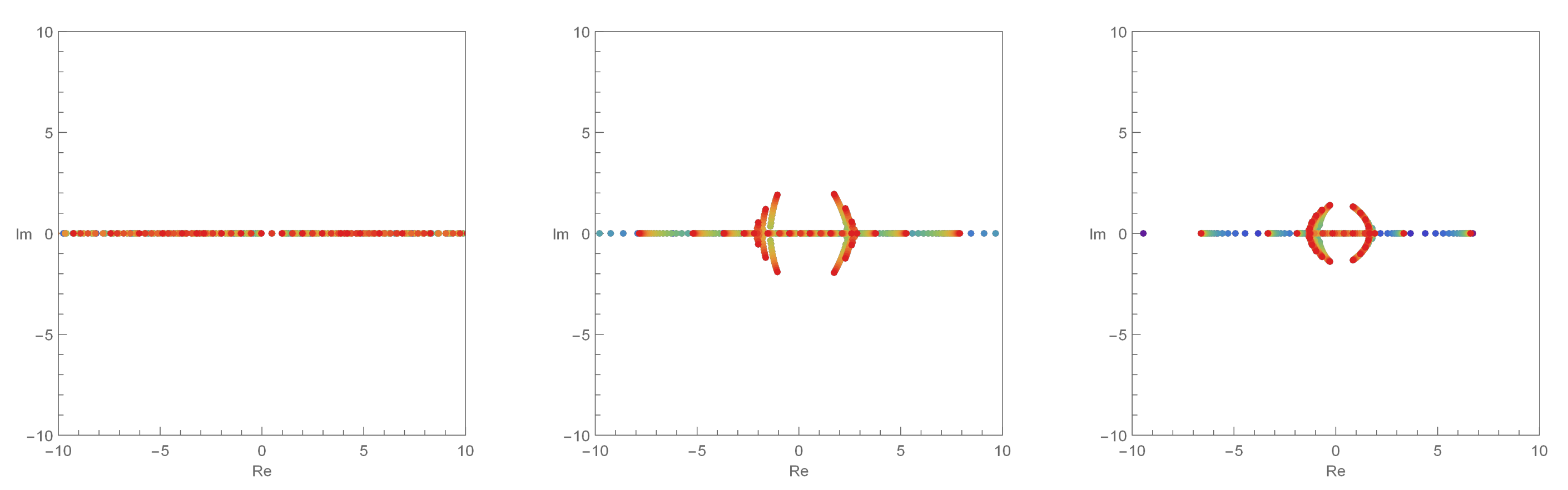
Figure 1 shows the structure of the approximate roots for q-cosine Euler polynomials. Let $y=7$ and $1\le n\le 30$. The left graph in Figure 1 is q=0.99, the middle graph is $q=0.9$, and the right graph is $q=0.8$. The blue color denotes that n is small, and the red color denotes that n is 30. In Figure 1, we show that the approximate roots of q-cosine Euler polynomials include all real numbers in $q=0.99$ when $n=30$. In addition, we conject that the approximate roots of q-cosine Euler polynomials show a circle structure near 0 when q approaches 0 and n continues to increase.

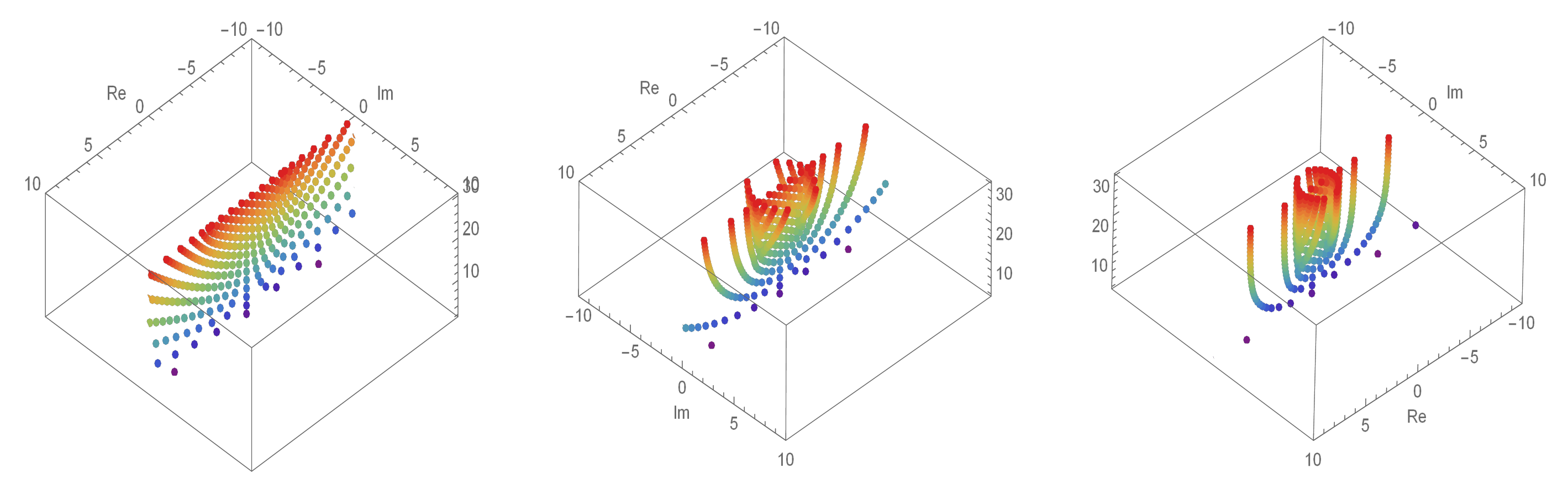
Figure 2 shows the 3D structure of Figure 1 under the same conditions. The left shape is the approximate roots of q-cosine Euler polynomials when $q=0.99$, $y=7$, and $1\le n\le 30$. This shape indicates that all the approximate roots are located on an imaginary axis. The middle shape in Figure 2 shows the approximate roots of q-cosine Euler polynomials when $q=0.9$, $y=7$, and $1\le n\le 30$. Here, we can observe the movement of the approximate roots. When $q=0.8$ and $y=7$, we can see the right shape of Figure 2. The shape variation in Figure 2 implies that the approximate roots change to imaginary numbers from real numbers and that the root structure for q-cosine Euler polynomials vary according to q.

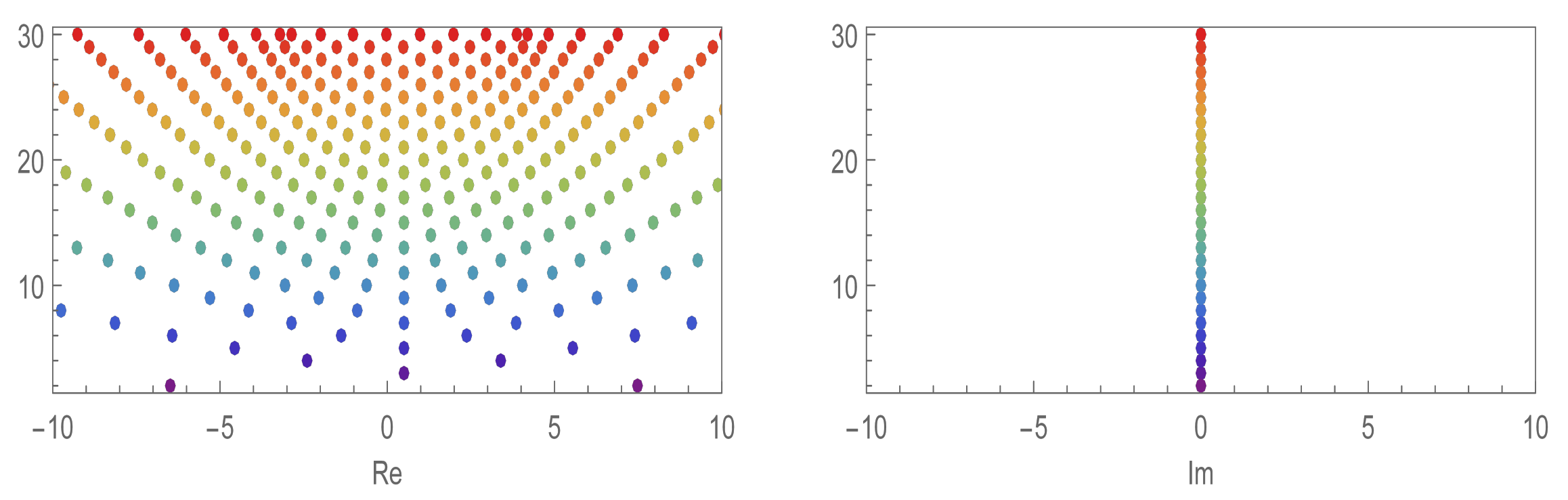
Conjecture 1.

If n increases and $q\to 0$, then the approximate roots of q-cosine Euler polynomials display a circle shape near the origin except for some zeros.

In Figure 3, $q=0.99$ and $y=7$ when $1\le n\le 30$. Under these conditions, we observe that the approximate roots of q-cosine Euler polynomials have a symmetric property and include all real numbers. By observing the right graphs in Figure 1 and Figure 3, we can consider Conjecture 2.

Conjecture 2.

Prove that ${}_C{\mathcal{E}}_{n,q}(x,y)$ is reflection symmetry analytic complex functions which has $\mathrm{Re}\left(x\right)=1/2$ in addition to the usual $\mathrm{Im}\left(x\right)=0$, when y is a fixed point in real numbers.

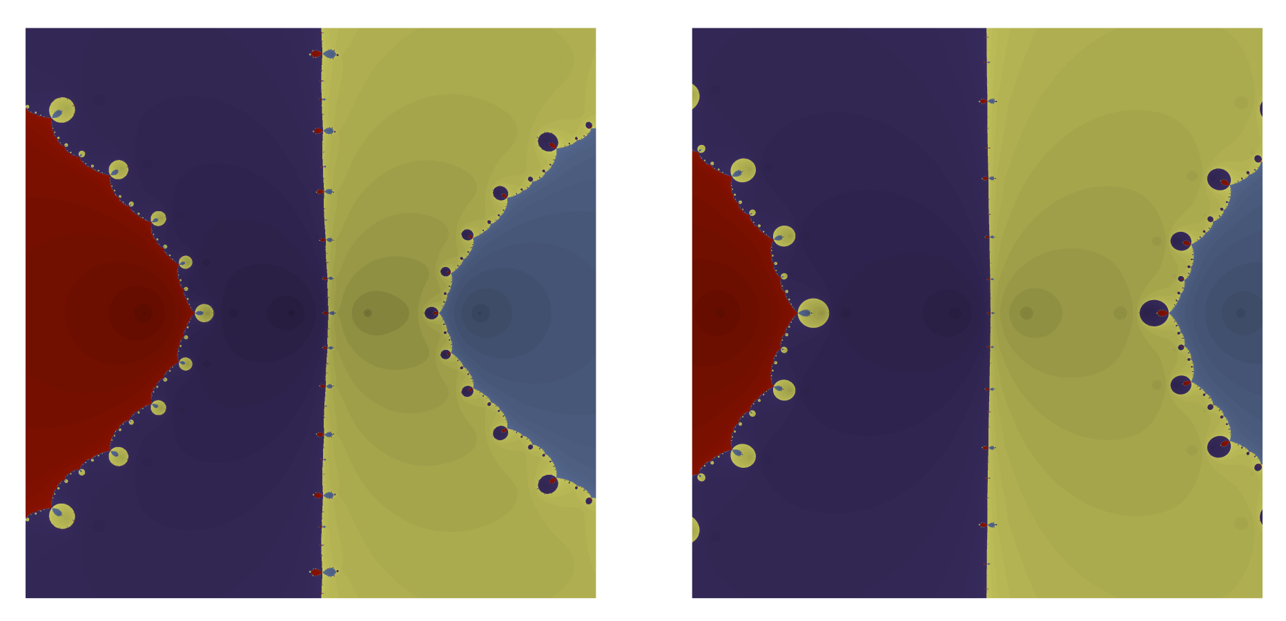
By using the Newton’s method(see [22]), we see the following Example 1. The equation of the left figure in Example 3 is $1.1965181875000004+2.912903125000001x-5.745637500000002x^2-0.5555x^3+x^4$, that is $q=0.1$. In Table 1, we note that the approximate roots are $-2.33937,-0.271276,0.795233,$ and $2.37091$, where $q=0.1$ and $y=7$. When we choose $-4\le \mathrm{Re}\left(x\right)\le 4$ and $-4\le \mathrm{Im}\left(x\right)\le 4$, we obtain the left figure in a complex plane. The complex numbers in the red, violet, yellow, and sky-blue ranges move to $-2.3397$, $-0.271276$, $0.795233$, and $2.37091$, respectively. The right figure in Example 3 illustrates the 4-th q-cosine Euler polynomials when $q=0.5$ and $y=7$. Numbers of the red, violet, yellow, and sky-blue ranges in the complex plane become $-7.20113$, $-0.610105$, $1.36484$, and $7.3839$, respectively (Figure 4).

Example 3.

The 4-th q-cosine Euler polynomials display the following figures in a complex plane:

5. Conclusions

In this paper, we have identified several properties of q-cosine Euler polynomials and q-sine Euler polynomials. In addition, the relationship between polynomials was confirmed according to the various conditions of the variables. We were able to assume the structure of the approximate roots of the q-cosine Euler polynomials and the q-sine Euler polynomials and finally, produce some speculations. The structure of the approximate roots will come out in various ways depending on the condition of the variables, and new methods and theorems related to approaching this needs to be created and proved.