Article

Color Image Quantization Based on the Artificial Bee Colony and Accelerated K-means Algorithms

Department of Computer Science, National Pingtung University, Pingtung City, Pingtung County 90003, Taiwan
Symmetry 2020, 12(8), 1222; https://doi.org/10.3390/sym12081222
Submission received: 20 June 2020 / Revised: 15 July 2020 / Accepted: 23 July 2020 / Published: 25 July 2020
(This article belongs to the Section Computer)

Abstract

:
Color image quantization techniques have been widely used as an important approach in color image processing and data compression. The key to color image quantization is a good color palette. A new method for color image quantization is proposed in this study. The method consists of three stages. The first stage is to generate N colors based on 3D histogram computation, the second is to obtain the initial palette by selecting K colors from the N colors based on an artificial bee colony algorithm, and the third is to obtain the quantized images using the accelerated K-means algorithm. In order to reduce the computation time, the sampling process is employed. The closest color in the palette for each sampled color pixel in the color image is efficiently determined by the mean-distance-ordered partial codebook search algorithm. The experimental results show that the proposed method can generate high-quality quantized images with less time consumption.

1. Introduction

Color image quantization is one of the digital image processing techniques [1]. Color image quantization consists of two steps. The first step is to generate a set of representative colors in order to obtain a color palette. The second is to map each pixel in the color image to one color in the color palette. The main purpose of color image quantization is to reduce the storage requirements and the transfer time of the image.
Hsieh and Fan [2] proposed a method for color image quantization based on an adaptive clustering algorithm and a pixel-mapping algorithm. Omran et al. [3] developed a color image quantization algorithm based on particle swarm optimization and the K-means algorithm. The main disadvantage of their method is the high computational cost. Hu and Lee [4] introduced the use of stable flags for palette entries in order to accelerate the K-means algorithm for palette design. Celebi [5] implemented the fast and exact variants of K-means with several initialization schemes. Su and Hu [6] proposed a color image color quantization algorithm based on self-adaptive differential evolution. El-Said [7] proposed a fuzzy clustering algorithm, which combines the artificial fish swarm algorithm and an efficient extension of fuzzy c-means (FCM), for color image quantization. Schaefer and Nolle [8] introduced a new approach to color image quantization. In their method, the color palette is derived by the simulated annealing algorithm in order to provide good image quality according to S-CIELAB. In 2015, a color quantization method, called ATCQ, was proposed by Pérez-Delgado [9]. ATCQ adapted some of the features of the basic Ant-tree to obtain a quicker algorithm for color image quantization. Ueda et al. [10] described a modification of the median cut algorithm. In their method, a combination of linear discriminant analysis and principal analysis was used to accomplish effective partitioning of the color space. In 2019, application of the shuffled-frog leaping algorithm to perform color image quantization was proposed by Pérez-Delgado [11]. Each frog represented a quantized palette and the objective function considered is the mean square error.
Although some existing methods can obtain high-quality quantized images, these methods suffer from the drawback of high computational cost. In order to obtain the quantized images with high image quality and low computational cost, a color image quantization technique is proposed in this study. Experimental results show that the proposed method can generate high-quality quantized images with less time consumption.
The rest of this paper is organized as follows. In Section 2, some related works are reviewed. In Section 3, the color image quantization method is described. In Section 4, some experimental results are presented. Finally, some conclusions are given in Section 5.

2. Related Works

In this section, the artificial bee colony algorithm and the mean-distance-ordered partial codebook search algorithm will be reviewed.

2.1. Artificial Bee Colony (ABC) Algorithm

The artificial bee colony algorithm [12,13,14,15,16,17,18,19,20,21,22] was first proposed by Karaboga and was inspired by the foraging behaviors of bee colonies. In this study, the number of food sources is denoted by SN, and the position of a food source represents a possible solution to the optimization problem. Each solution si (i = 0, 1, 2, …, SN − 1) is a K-dimensional vector. Here, K is the color number of a color palette.
In the employed bee phase, a new solution vi is produced by the i-th employed bee as follows:
v i , j = s i , j + φ i j ( s i , j s t , j )
where st is a food source selected randomly, j is selected from the set {0, 1, 2, …, K − 1}, and φ i j is a random number within the range [−1, 1]. In the onlooker bee phase, each onlooker bee selects a food source depending on probi which is calculated by the following expression:
p r o b i = f i t n e s s ( s i ) j = 0 S N 1 f i t n e s s ( s j )
where fitness(si) is the fitness value of the solution si. Then, the onlooker bees try to improve the solutions by using Equation (1).
The main steps of the ABC algorithm (Algorithm 1) are shown as follows:
Algorithm 1: ABC algorithm [12]
 Step 1: Generate the initial population si, i = 0, 1, 2, …, SN − 1
   triali = 0, i = 0, 1, 2, …, SN − 1. In the ABC algorithm, trial is a vector holding trial numbers
   through which solutions cannot be improved
   Set cycle to 1
 Step 2: Evaluate the fitness fitness(si) of the population and memorize the best solution so far
Repeat
 Step 3: Employed bee phase
 Step 4: Compute the values probi (i = 0, 1, 2, …, SN − 1) by using Equation (2)
 Step 5: Onlooker bee phase
 Step 6: Memorize the best solution so far
 Step 7: Scout bee phase
  cycle = cycle + 1
Until cycleABC_cycle

2.2. Mean-Distance-Ordered Partial Codebook Search (MPS) Algorithm

The MPS algorithm is a fast search algorithm for vector quantization [23,24]. Here, the MPS algorithm is employed to achieve reduction in computation time for color image quantization. For each color pixel in the color image, the closest color in the palette can be efficiently determined by the MPS algorithm.
For the color pixel x and the palette color c in the palette, the squared Euclidean distance (SED) and the squared sum distance (SSD) are defined as follows.
S E D ( x , c )   =   j = 1 3 ( x j c j ) 2
S S D ( x , c )   =   ( j = 1 3 x j j = 1 3 c j ) 2
The following inequality that holds true for the color pixel x and the palette color c is described as follows [23]:
S S D ( x , c )     3 × S E D ( x , c )
In the MPS algorithm, the test condition was employed to reject some impossible palette colors:
3 × d min   <   S S D ( x , c )
where dmin denotes the minimal SED between the color pixel x and the closest color cmin found so far. The inequality dmin < SED(x,c) can be derived from Equations (5) and (6), and thus the palette color c cannot be the closest color.
If the color pixel x = (100, 50, 80), the sorted palette of K colors is as depicted in Figure 1a. In this study, the initial searched palette color for the color pixel x is the palette color with the closest mean value to x. The initial searched palette color can be found by the binary search technique. In this case, the palette color with the closest mean value to x is (101, 52, 78); therefore, the searching order of colors in the palette is depicted in Figure 1b.
It is noted that the MPS test condition has two properties. Here, mean (c), mean (c1), and mean (x) denote the mean value of palette color c, the mean value of palette color c1, and the mean value of color pixel x, respectively. The first property is that if mean (c) is less than mean (x), when the palette color c is rejected, the palette color c1 is also rejected if mean (c1) is less than mean (c). The second property is that if mean (c) is greater than mean (x), when the palette color c is rejected, the palette color c1 is also rejected if mean (c1) is greater than mean (c).

3. Proposed Color Image Quantization Algorithm

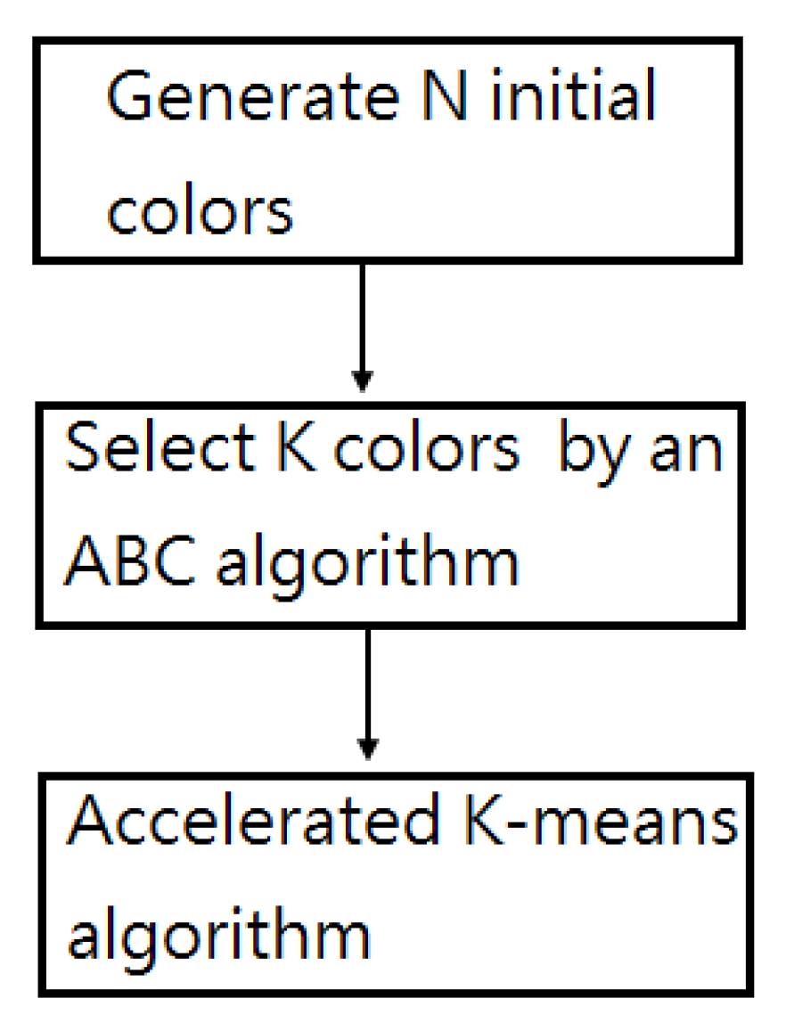
The method consists of three stages. The system flowchart is shown in Figure 2. The three stages are described in this section.

3.1. Generate N Initial Colors

The RGB color system is adopted in this study. The R, G and B values range from 0 to 255. For the Lake image, Figure 3 shows its 3D histogram. The RGB values of each pixel in an image correspond to a point of its 3D histogram. In the proposed scheme, the 3D RGB space is divided into non-overlapping cubes, and the size of each cube is 16 × 16 × 16. There are (256 × 256 × 256)/(16 × 16 × 16) = 4096 cubes in total. It is observed that many cubes contain no point. If the point number contained in the cube is equal to or larger than the threshold PixelThr, then the cube will be preserved. Assume that the number of the preserved cube is N. The point number contained in the i-th preserved cube is denoted by initialn[i] (i = 0, 1, 2, …, N − 1), and the center of all the points in the i-th preserved cube is denoted by initialc[i]. The colors initialc[0], initialc[1], …,initialc[N − 1] are called the N initial colors.
For example, there are 8 cubes shown in Figure 4, and they contain 0, 0, 10, 1, 0, 12, 2, and 0 points, respectively. Assume the value of PixelThr is set to 5. Cubes 2 and 5 will be preserved because the point numbers contained within them are equal to or larger than 5. Hence, the values of N, initialn[0] and initialn[1] are 2, 10 and 12, respectively. The center of the 10 points contained in cube 2 is called initialc[0]. Consequently, the center of the 12 points contained in cube 5 is called initialc[1].

3.2. Select K Colors by an ABC Algorithm

In this study, an ABC algorithm is employed to select K colors from the N initial colors to form the initial palette. The basic components of the artificial bee colony algorithm for solving this problem are described in the following subsections.

3.2.1. Representation of Solutions and Fitness Function

The proposed method considers the N initial colors and their corresponding point numbers in order to generate the initial palette. In the initialization phase, the SN solution si (i = 0, 1, 2, …, SN − 1) is generated, where si = (si,0, si,1, si,2,…, si,K−1), si,j is an integer number and the 0 ≤ si,j < si,j+1N − 1 for j = 0, 1, 2,…, K − 2. Solution si indicates that the set of initial palette colors is {initialc[si,0], initialc[si,1], initialc[si,2], …,initialc[si,K−1]}. Then, the fitness, fitness(si), of a solution si is defined as
f i t n e s s ( s i ) = 1 1 + M S E 1   , M S E 1 = j = 0 N 1 i n i t i a l n [ j ] × D ( i n i t i a l c [ j ] , s i ) j = 0 N 1 i n i t i a l n [ j ]   ,
where D(initialc[j], si) = min{SED(initialc[j], initialc[si,0]), SED(initialc[j], initialc[si,1]), …, SED(initialc[j], initialc[si,K−1])}.

3.2.2. Generation of a New Solution vi

As described in Section 2.1, the structure of the original ABC is suitable for continuous problems. Thus, Equation (1) needs to be modified for this specific problem. Let si = (si,0, si,1, si,2, …, si,K−1) be the present solution, while st = (st,0, st,1, st,2, …,st,K−1) is the randomly selected solution. The proposed method will generate the new solution vi. The new solution vi is the same as si except that si,j is replaced by vi,j, where j is selected from the set {0, 1, 2,…, K − 1}.
The value of vi,j (Algorithm 2) is computed by the following steps:
Algorithm 2: The steps of computing the value of vi,j
Step 1: Range1 = si,j − abs(si,j − st,j),
   Range2 = si,j + abs(si,j − st,j),
    If (Range1 < 0) { Range1 = 0; }
    If (Range2 > (N − 1)) { Range2 = N − 1; }
Step 2: SetX = {};
   for (y = Range1; yRange2; y++)
     { If (y is not an element of si) SetX = SetX ∪ {y}; }
Step 3: If (SetX == {}) { vi,j = si,j; }
    else { Assume SetX = { y0, y1, …, ym−1}, the probability of the value of vi,j is set to yr being
      initialn(yr)/(initialn[y0] + initialn[y1] +… + initialn[ym−1]) for r = 0, 1, …, m − 1; }

3.2.3. The Search Process

In the employed bee phase, the i-th employed bee produces a new solution vi by the method described in Section 3.2.2. If fitness(vi) > fitness(si) then si is replaced by vi and triali is set to 0 else triali = triali + 1. In the onlooker bee phase, each onlooker bee which selects a solution si depending on probi also produces a new solution vi by the method described in Section 3.2.2. If fitness(vi) > fitness(si) then si is replaced by vi and triali is set to 0 else triali = triali+1. In the scout bee phase, the scout bee randomly produces the new solution to replace si if the triali of solution si is more than the parameter ‘limit’. In this study, the value of the parameter ‘limit’ is set to 10. The ABC algorithm is finished if the criterion cycle > ABC_cycle is satisfied. The best solution found so far is output and it represents the initial palette in this study.
In the second stage, the criterion N K must be satisfied. If the value of N obtained is less than the value of K, the proposed method will decrease the value of PixelThr in order to satisfy the criterion N K. When the value of PixelThr is set to 1 and the value of N obtained is less than the value of K, the proposed method will skip the second stage and set K = N. That is, the color number of a color palette is N.

3.3. Accelerated K-means Algorithm

The K-means algorithm is the most commonly used algorithm for data clustering. It is found that the computational cost of the K-means algorithm for color image quantization is very high. Hence, the accelerated K-means algorithm is employed for color image quantization in this study.
In order to achieve reduction in computation time, the sampling process is employed in this study. First, the color image is divided into many non-overlapping blocks. When every pixel of the color image is sampled it indicates that the sampling rate = 1, when only one pixel is sampled for a 2 × 2 block it indicates that the sampling rate = 0.25, when only two pixels are sampled for a 4 × 4 block it indicates that the sampling rate = 0.125, and when only one pixel is sampled for a 4 × 4 block it indicates that the sampling rate = 0.0625. Then, the sampled pixels and the initial palette serve as the input of the accelerated K-means algorithm. Detailed descriptions of the accelerated K-means algorithm (Algorithm 3) for color image quantization are given below.
Algorithm 3: Accelerated K-means algorithm for color image quantization
Step 1: The initial palette is generated by selecting K colors from the N initial colors based on an
   ABC algorithm.
   Set cycle to 1
Step 2: For each sampled color pixel in the color image, the closest color in the palette is efficiently
   determined by the MPS algorithm. If the index value of its closest palette color is j, the
   sampled color pixel is classified into the j-th group.
Step 3: The mean values of these K groups are computed. These K values are sorted in the
   ascending order of their means in order to generate the new color palette.
   cycle = cycle + 1
Step 4: If the stopping criterion cycle > K_means_cycle is satisfied, then the algorithm stops.
   Otherwise, go to Step 2.

4. Experimental Results

The proposed algorithm was implemented in C language and executed on a PC running under the operating system of Windows 7 with Intel Core 3.6 GHz CPU and 32 GBytes of RAM. The five color images Lena, Baboon, Lake, Peppers and Airplane with a size of 512 × 512 were used for conducting the experiments. The following parameters were used in the experiments: PixelThr = 30, SN = 20, ABC_cycle = 15 and K_means_cycle = 20.
In the experiments, the proposed algorithm was executed 20 times for each given image. Table 1 shows the experimental results. The results presented are the solutions with the average mean square error, the standard deviation (S.D.), and average computation time. The mean square error (MSE) was defined as follows:
M S E = 1 512 × 512 i = 0 511 j = 0 511 S E D ( f ( i , j ) , f ( i , j ) ) ,
where f is the original color image, and f′ is the quantized image. It was observed that when K increased, the average mean square error decreased and the average computation time increased. When the sampling rate increased, the average computation time increased for all cases, and the average mean square error decreased in most cases.
In the proposed method, the total computation time was the summation of computation time for initial palette generation and computation time for clustering by the accelerated K-means algorithm. Table 2 shows the computation time for color image quantization. These results were obtained by the proposed method with a sampling rate of 0.125. It was observed that the computation time for initial palette generation always increased with the increase in K. Similarly, the computation time for clustering by accelerated K-means algorithm always increased with the increase in K.
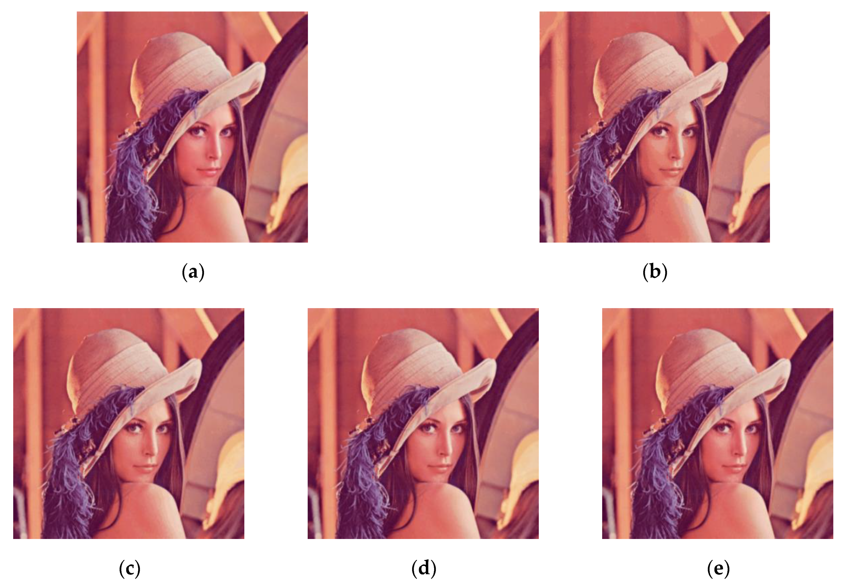
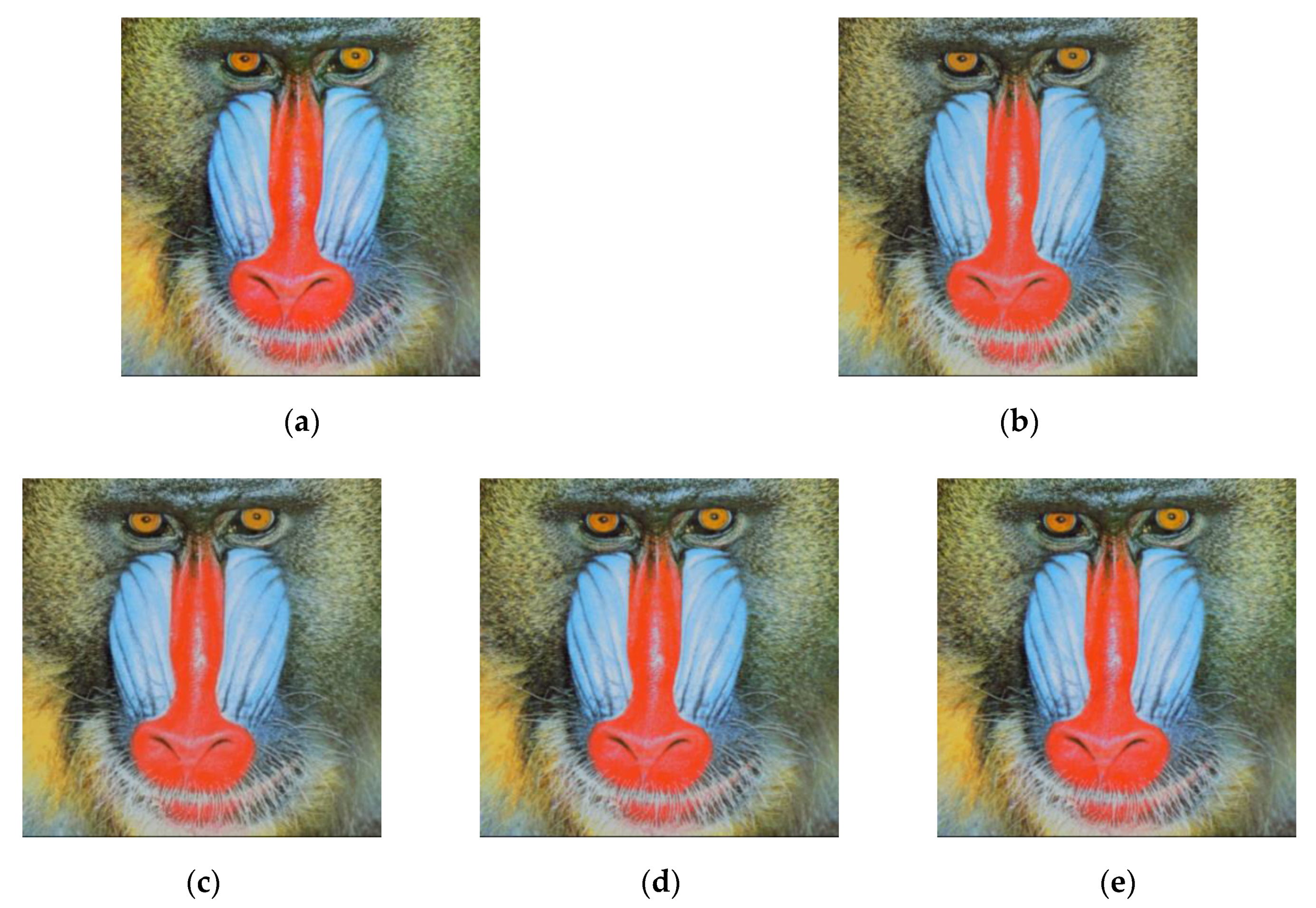
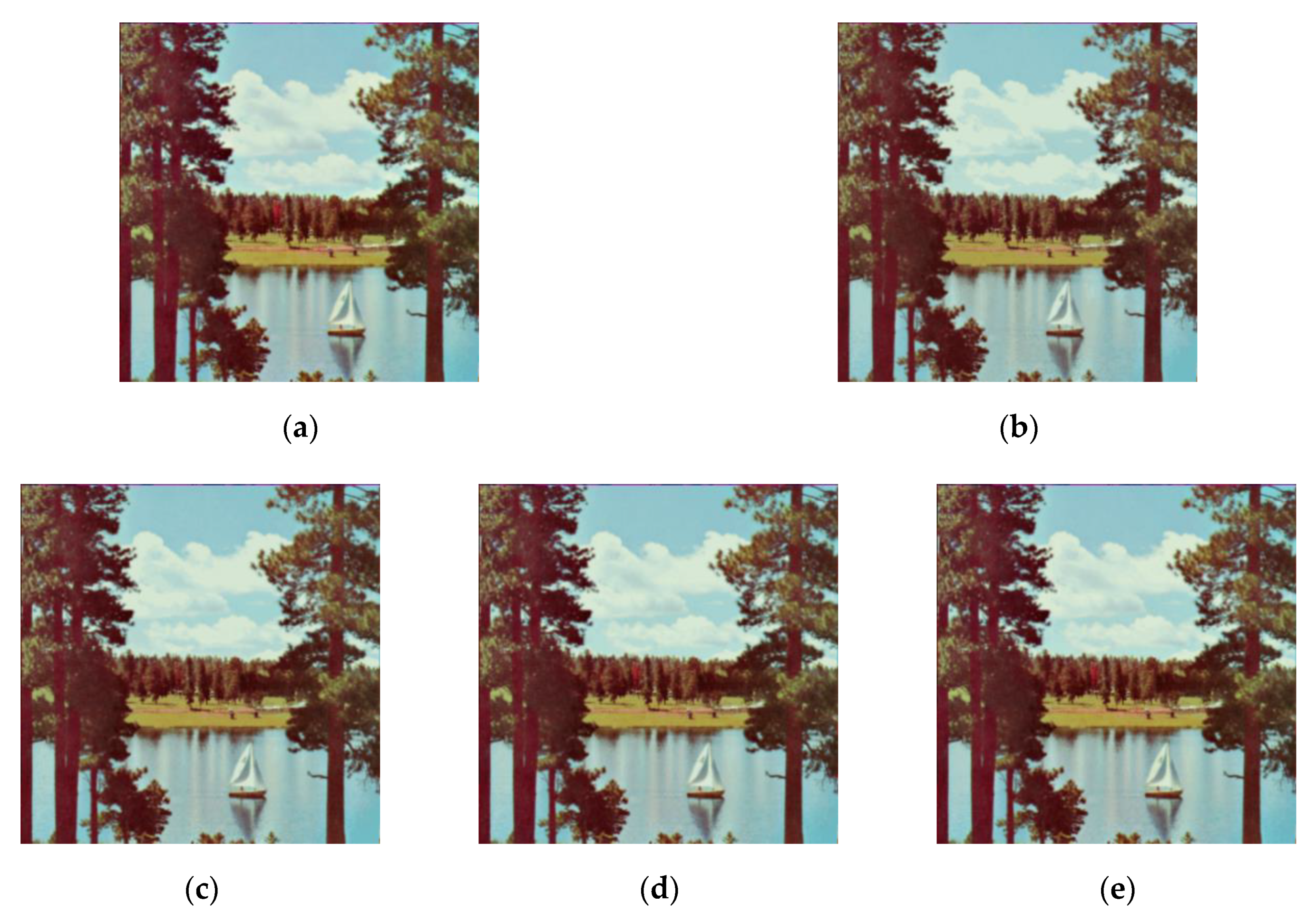
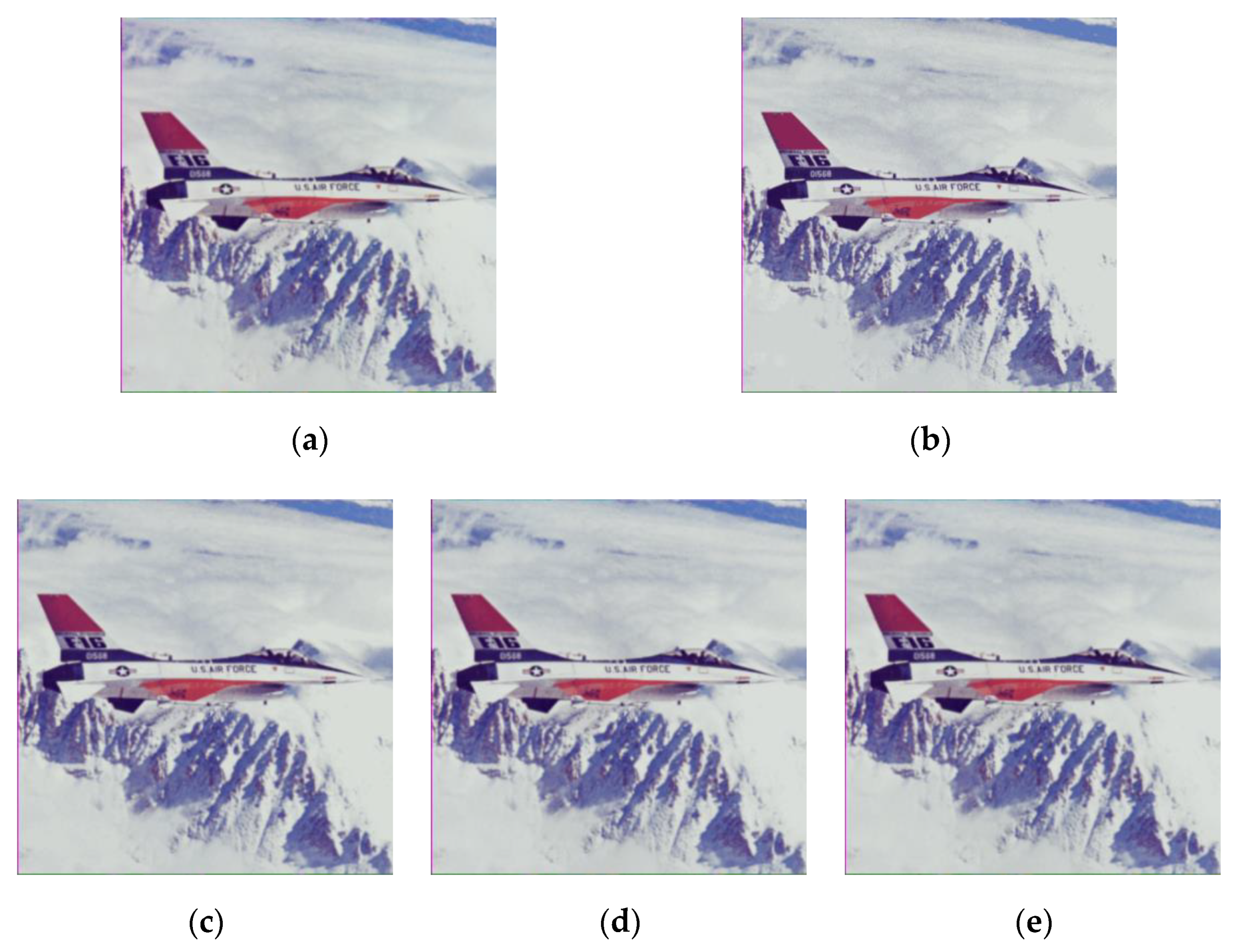
Figure 5, Figure 6, Figure 7, Figure 8 and Figure 9 illustrate the quantized images of Lena, Baboon, Lake, Peppers, and Airplane, respectively, corresponding to K = 32, 64, 128 and 256. These figures were obtained by the proposed method with a sampling rate of 0.125. It shows that the proposed method can generate high-quality quantized images. We can observe that there is no visual difference between the original and the 256 colors quantized images. In Figure 8a, there is a red tree in the middle region. However, the color of this tree is not red in Figure 8b. That is, there are some visual differences between the original and the 32 colors quantized images.

4.1. The Effect of the Algorithm Parameters

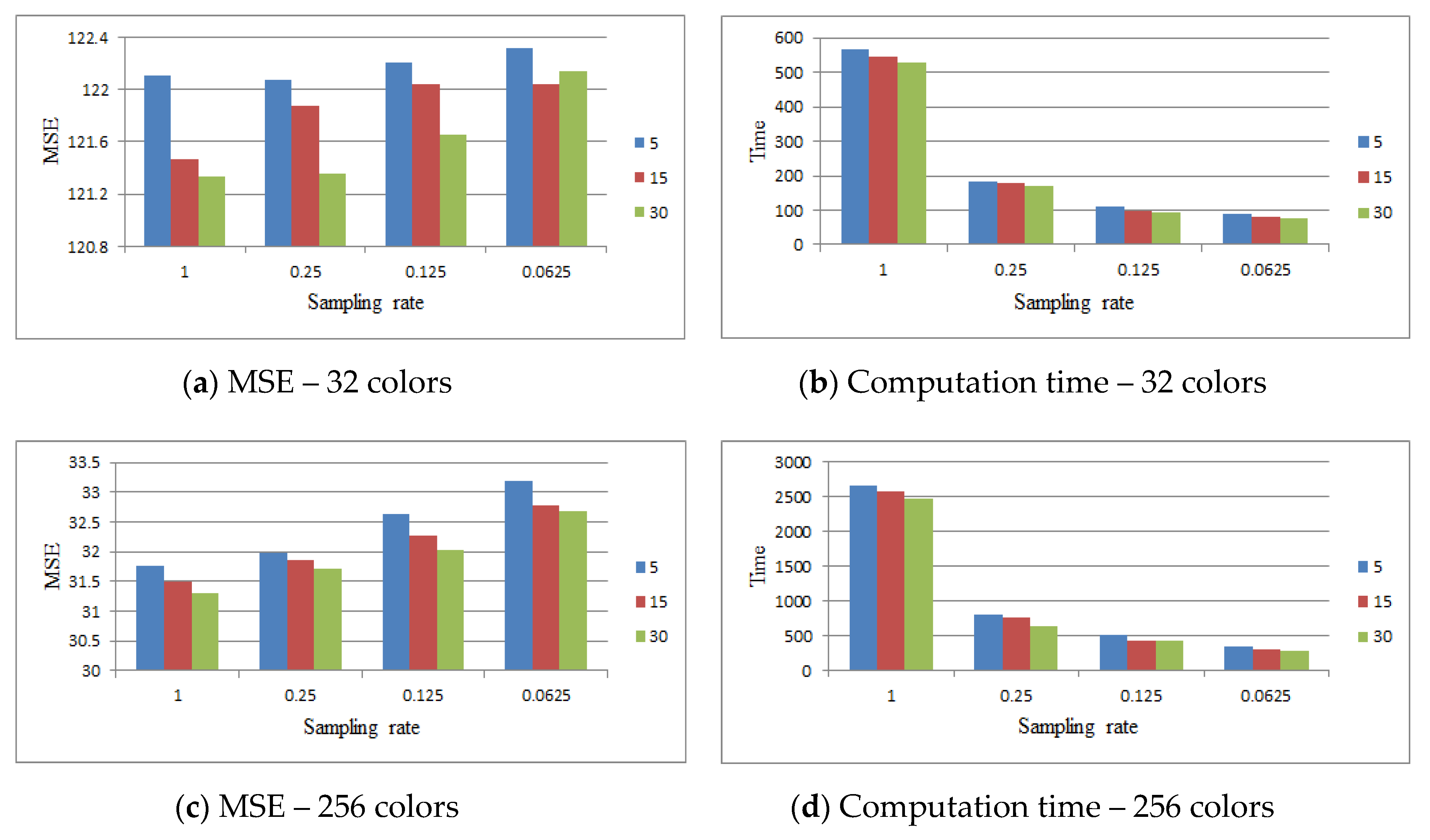
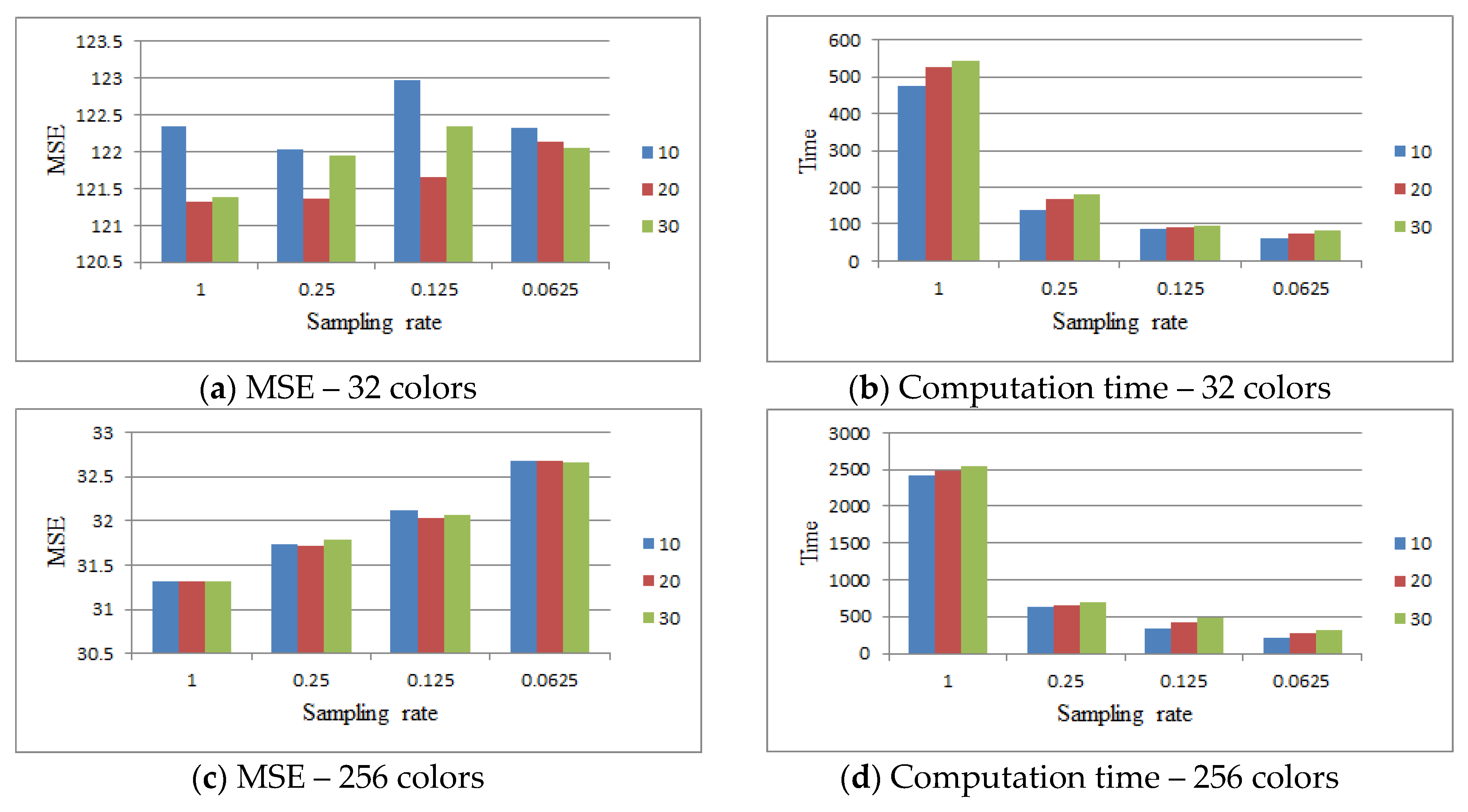
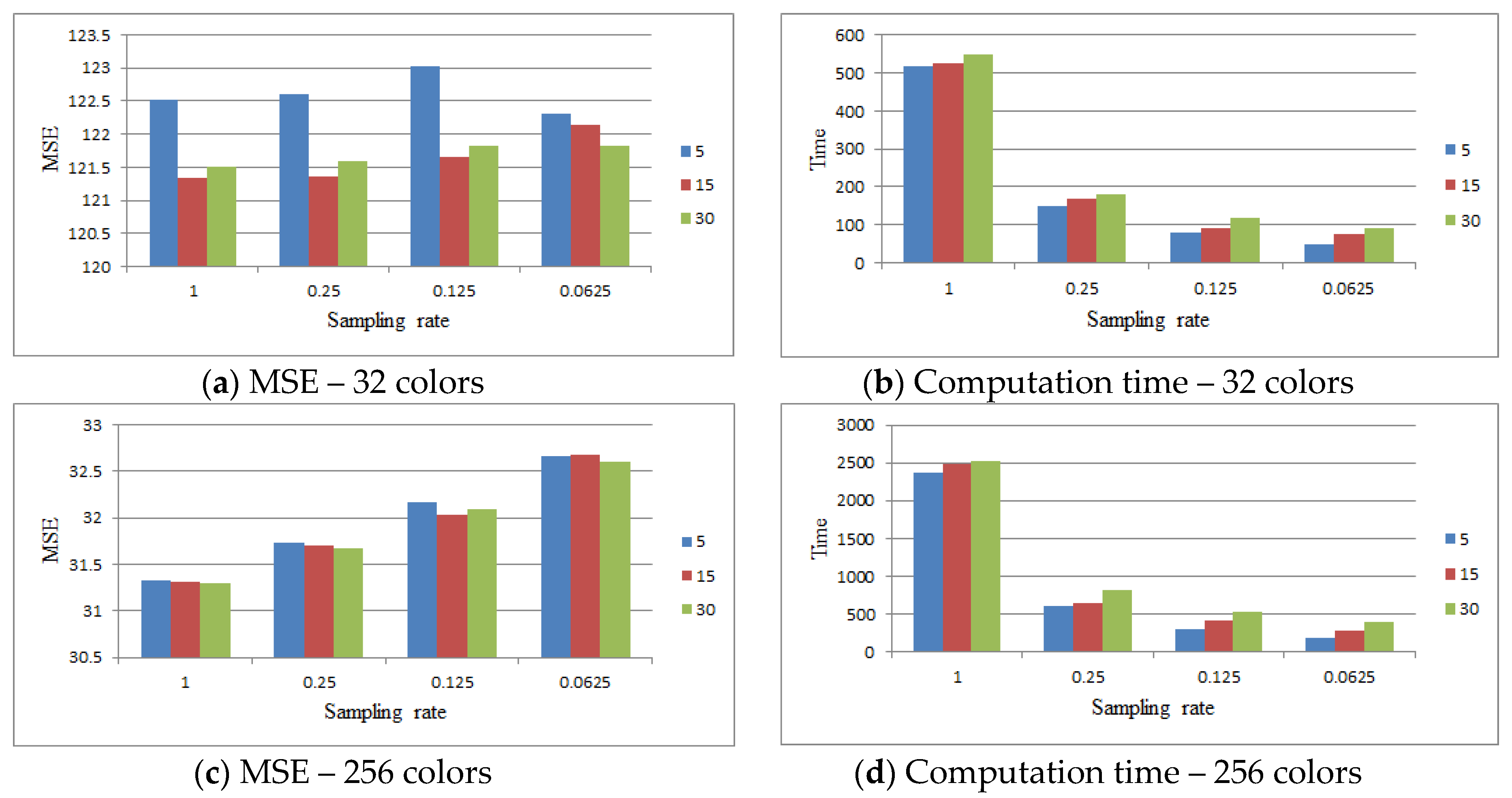
This subsection analyzes the effect of the algorithm parameters on the solution. The comparison was applied to the Lena image quantized to 32 and 256 colors. The following parameters were used in the experiments: PixelThr = 30, SN = 20, ABC_cycle = 15 and K_means_cycle = 20. When a parameter was analyzed, the other parameters remained unchanged, and the average MSE and the average computation time (milliseconds) obtained will be shown in a figure for comparison.
As described in Section 3.1, the 3D RGB space was divided into non-overlapping cubes, and the size of each cube was 16 × 16 × 16. If the point number contained in the cube was equal to or larger than the threshold PixelThr, then the cube was preserved. The number of the preserved cube was N in this study. Figure 10 compares the results of PixelThr = {5, 15, 30}. This figure shows that as PixelThr increased, the computation time decreased slightly for all cases. When PixelThr increased, the MSE value decreased slightly in most cases.
SN is the number of food sources in the ABC algorithm. The ABC algorithm was employed to select K colors from the N initial colors to form the initial palette in this study. Figure 11 compares the results of SN = {10, 20, 30}. This figure shows that as SN increased, the computation time increased slightly for all cases. It was observed that the MSE value does not always decrease with the increase in SN.
The ABC algorithm was finished if the criterion cycle > ABC_cycle was satisfied. Figure 12 compares the results of ABC_cycle = {5, 15, 30}. This figure shows that as ABC_cycle increased, the computation time increased slightly for all cases. It was observed that the MSE value does not always decrease with the increase in ABC_cycle.
In the accelerated K-means algorithm, the algorithm stops if the criterion cycle > K_means_cycle is satisfied. Figure 13 compares the results of K_means_cycle = {5, 10, 20}. This figure shows that as K_means_cycle increased, the computation time increased and the average MSE decreased for all cases.

4.2. Comparison with the Method Proposed by Pérez-Delgado

In 2019, the application of the shuffled-frog leaping algorithm to perform color quantization was proposed by Pérez-Delgado [11], and this method is identified as SFLA-CQ. The SFLA-CQ algorithm was coded in C language and executed on a PC running under the Linux operating system with 8 GBytes of RAM and an AMD Ryzen 7 1800X Turbo processor (4.0 GHz). Table 3 shows the results obtained by SFLA-CQ.
The performance of the proposed method with sampling rate = 0.125 was compared to SFLA-CQ with sampling rate = 0.1. For the Lena image, the average MSE obtained by the proposed method was near to that obtained by SFLA-CQ. For the Baboon image, the average MSE obtained by the proposed method was slightly higher than that obtained by SFLA-CQ. For the Pepper and Lake images, the average MSE obtained by the proposed method was slightly lower than that obtained by SFLA-CQ when K = 64, 128 and 256. For the Airplane image, the average MSE obtained by the proposed method was lower than that obtained by SFLA-CQ. These results clearly show that the computation time of SFLA-CQ is greater than that of the proposed method.
In summary, the proposed method can generate high-quality quantized images. These results reveal that the proposed method is superior to SFLA-CQ in terms of average computation time.

5. Conclusions

A new method is presented for color image quantization in this study. The method consists of three stages. The first stage is to generate N colors based on 3D histogram computation, the second is to obtain the initial palette by selecting K colors from the N colors based on an ABC algorithm, and the third is to obtain the quantized images using the accelerated K-means algorithm. In order to achieve reduction in computation time, the sampling process and the MPS algorithm are employed in this study.
Experimental results show that the proposed method can generate high-quality quantized images. When the sampling rate = 0.125, the average computation time of the proposed method is less than 1 s for all cases. The main contributions of this paper are that the proposed method can generate high-quality quantized images with less time consumption, and the experimental results reveal the feasibility of the proposed approach.

Funding

This research received no external funding.

Acknowledgments

This work was supported by the Ministry of Science and Technology, Taiwan, under Grant MOST 104-2221-E-153-012.

Conflicts of Interest

The author declares that there is no conflict of interest.

References

  1. Gonzalez, R.C.; Woods, R.E. Digital Image Processing, 4th ed.; Pearson: New York, NY, USA, 2018. [Google Scholar]
  2. Hsieh, I.S.; Fan, K.C. An adaptive clustering algorithm for color quantization. Pattern Recognit. Lett. 2000, 21, 337–346. [Google Scholar] [CrossRef]
  3. Omran, M.G.; Engelbrecht, A.P.; Salman, A. A color image quantization algorithm based on particle swarm optimization. Informatica 2005, 29, 261–269. [Google Scholar]
  4. Hu, Y.C.; Lee, M.G. K-means-based color palette design scheme with the use of stable flags. J. Electron. Imaging 2007, 16. [Google Scholar] [CrossRef]
  5. Celebi, M.E. Improving the performance of k-means for color quantization. Image Vis. Comput. 2011, 29, 260–271. [Google Scholar] [CrossRef] [Green Version]
  6. Su, Q.; Hu, Z. Color image quantization algorithm based on self-adaptive differential evolution. Comput. Intell. Neurosci. 2013, 2013. [Google Scholar] [CrossRef] [Green Version]
  7. El-Said, S.A. Image quantization using improved artificial fish swarm algorithm. Soft Comput. 2015, 19, 2667–2679. [Google Scholar] [CrossRef]
  8. Schaefer, G.; Nolle, L. A hybrid color quantization algorithm incorporating a human visual perception model. Comput. Intell. 2015, 31, 684–698. [Google Scholar] [CrossRef]
  9. Pérez-Delgado, M.L. Colour quantization with ant-tree. Appl. Soft Comput. 2015, 36, 656–669. [Google Scholar] [CrossRef]
  10. Ueda, Y.; Koga, T.; Suetake, N.; Uchino, E. Color quantization method based on principal component analysis and linear discriminant analysis for palette-based image generation. Opt. Rev. 2017, 24, 741–756. [Google Scholar] [CrossRef]
  11. Pérez-Delgado, M.L. Color image quantization using the shuffled-frog leaping algorithm. Eng. Appl. Artif. Intell. 2019, 79, 142–158. [Google Scholar] [CrossRef]
  12. Karaboga, D.; Basturk, B. A powerful and efficient algorithm for numerical function optimization: Artificial bee colony (ABC) algorithm. J. Glob. Optim. 2007, 39, 459–471. [Google Scholar] [CrossRef]
  13. Karaboga, D.; Basturk, B. On the performance of artificial bee colony (ABC) algorithm. Appl. Soft Comput. 2008, 8, 687–697. [Google Scholar] [CrossRef]
  14. Karaboga, D.; Akay, B. A comparative study of artificial bee colony algorithm. Appl. Math. Comput. 2009, 214, 108–132. [Google Scholar] [CrossRef]
  15. Karaboga, D.; Ozturk, C. Neural networks training by artificial bee colony algorithm on pattern classification. Neural Netw. World 2009, 19, 279–292. [Google Scholar]
  16. Karaboga, D.; Ozturk, C. A novel clustering approach: Artificial bee colony (ABC) algorithm. Appl. Soft Comput. 2011, 11, 652–657. [Google Scholar] [CrossRef]
  17. Draa, A.; Bouaziz, A. An artificial bee colony algorithm for image contrast enhancement. Swarm Evol. Comput. 2014, 16, 69–84. [Google Scholar] [CrossRef]
  18. Ozturk, C.; Hancer, E.; Karaboga, D. A novel binary artificial bee colony algorithm based on genetic operators. Inf. Sci. 2015, 297, 154–170. [Google Scholar] [CrossRef]
  19. Huang, S.C. High-quality codebook generation of vector quantization using the HT-ABC-LBG algorithm. J. Inf. Sci. Eng. 2018, 34, 81–102. [Google Scholar]
  20. Saad, E.; Elhosseini, M.A.; Haikal, A.Y. Culture-based artificial bee colony with heritage mechanism for optimization of wireless sensors network. Appl. Soft Comput. 2019, 79, 59–73. [Google Scholar] [CrossRef]
  21. Chen, X.; Tianfield, H.; Li, K. Self-adaptive differential artificial bee colony algorithm for global optimization problems. Swarm Evol. Comput. 2019, 45, 70–91. [Google Scholar] [CrossRef] [Green Version]
  22. Gorkemli, B.; Karaboga, D. A quick semantic artificial bee colony programming (qsABCP) for symbolic regression. Inf. Sci. 2019, 502, 346–362. [Google Scholar] [CrossRef]
  23. Ra, S.W.; Kim, J.K. A fast mean-distance-ordered partial codebook search algorithm for image vector quantization. IEEE Trans. Circuits Syst. II Analog. Digit. Signal. Process. 1993, 40, 576–579. [Google Scholar] [CrossRef]
  24. Hu, Y.C.; Su, B.H.; Tsou, C.C. Fast VQ codebook search algorithm for grayscale image coding. Image Vis. Comput. 2008, 26, 657–666. [Google Scholar] [CrossRef]
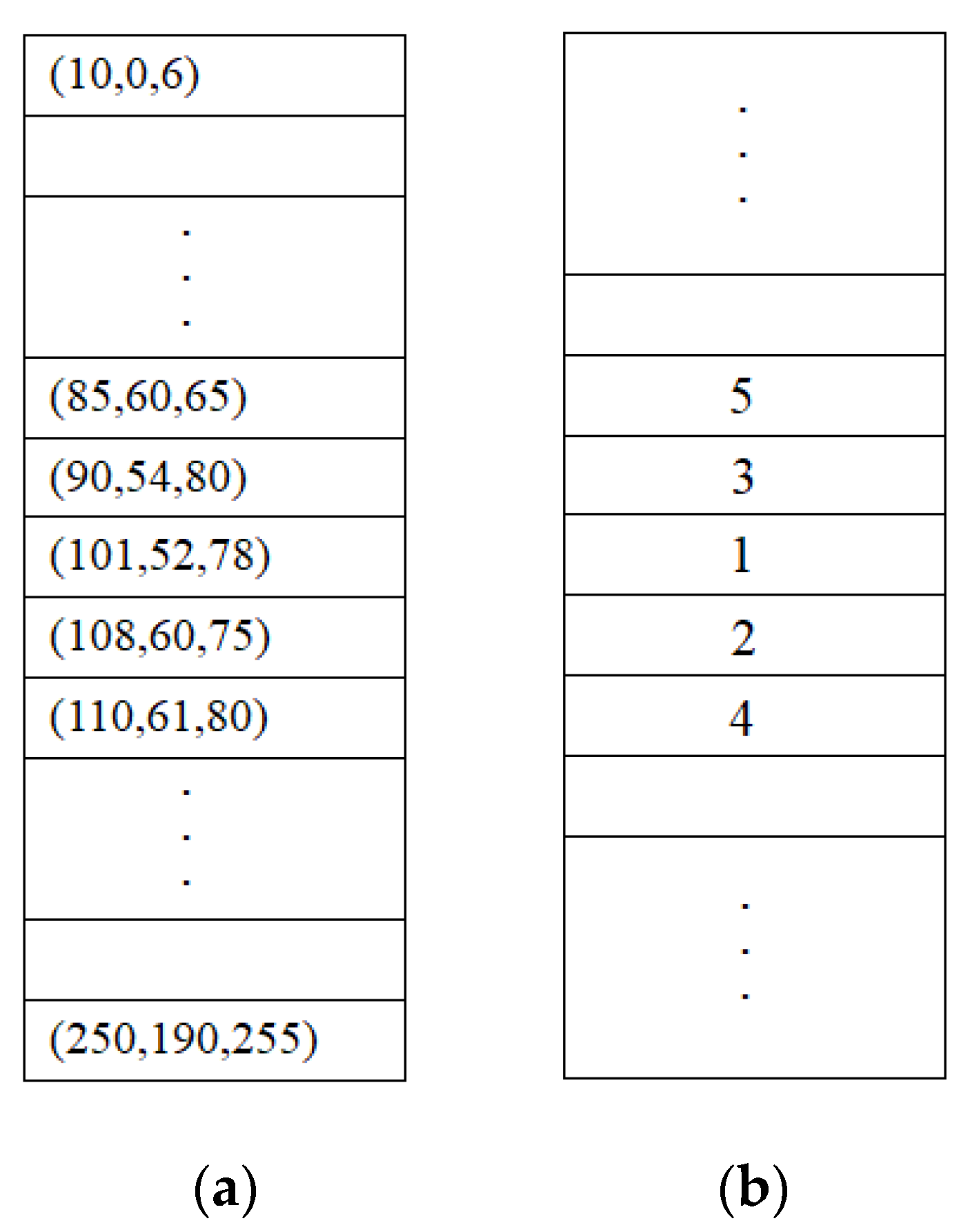
Figure 1. (a) The sorted palette of K colors; (b) the searching order of colors if the color pixel x = (100, 50, 80).
Symmetry 12 01222 g001
Figure 2. The system flowchart.
Symmetry 12 01222 g002
Figure 3. An example of a 3D histogram.
Symmetry 12 01222 g003
Figure 4. Cubes 0–7 contain 0, 0, 10, 1, 0, 12, 2, and 0 points, respectively.
Symmetry 12 01222 g004
Figure 5. (a) The Lena image, (b) 32 colors quantized image, (c) 64 colors quantized image, (d) 128 colors quantized image, (e) 256 colors quantized image.
Symmetry 12 01222 g005
Figure 6. (a) The Baboon image, (b) 32 colors quantized image, (c) 64 colors quantized image, (d) 128 colors quantized image, (e) 256 colors quantized image.
Symmetry 12 01222 g006
Figure 7. (a) The Pepper image, (b) 32 colors quantized image, (c) 64 colors quantized image, (d) 128 colors quantized image, (e) 256 colors quantized image.
Symmetry 12 01222 g007
Figure 8. (a) The Lake image, (b) 32 colors quantized image, (c) 64 colors quantized image, (d) 128 colors quantized image, (e) 256 colors quantized image.
Symmetry 12 01222 g008
Figure 9. (a) The Airplane image, (b) 32 colors quantized image, (c) 64 colors quantized image, (d) 128 colors quantized image, (e) 256 colors quantized image.
Symmetry 12 01222 g009
Figure 10. Comparing the results of PixelThr = {5, 15, 30} for the Lena image.
Symmetry 12 01222 g010
Figure 11. Comparing the results of SN = {10, 20, 30} for the Lena image.
Symmetry 12 01222 g011
Figure 12. Comparing the results of ABC_cycle = {5, 15, 30} for the Lena image.
Symmetry 12 01222 g012
Figure 13. Comparing the results of K_means_cycle = {5, 10, 20} for the Lena image.
Symmetry 12 01222 g013
Table 1. Results of the proposed method with PixelThr = 30, SN = 20, ABC_cycle = 15 and K_means_cycle = 20. (Sr: sampling rate, MSEa: average mean square error (MSE), T: average computation time (milliseconds)).
K = 32K = 64K = 128K = 256
ImageSrMSEaS.D.TMSEaS.D.TMSEaS.D.TMSEaS.D.T
Lena1.0121.331.5252773.841.0284847.530.53146031.310.122484
0.25121.361.6717074.130.8925247.660.4341431.710.14644
0.125121.661.839374.170.7315648.030.4823732.030.11422
0.0625122.141.327574.50.8111048.580.4116832.680.11275
Baboon1.0382.574.7835242.191.71226155.611.51962100.160.83259
0.25383.015.0260242.682.9413155.951.9677100.520.81145
0.125383.424.7193242.762.5273157.061.6461101.850.8783
0.0625387.064.3146244.461.9218158.061.4351103.440.8606
Peppers1.0236.773.2659141.734.0102986.453.3164455.460.42876
0.25237.313.0207141.953.933186.513.553956.050.4908
0.125237.874.6129141.722.720987.373.331856.810.3565
0.0625239.286.987143.033.513788.343.223758.070.4408
Lake1.0207.733.2651134.881.6100187.411.4153857.090.52665
0.25208.382.6217135.191.634388.581.151457.710.6818
0.125208.953.6120135.831.819289.10.931658.570.8532
0.0625210.293.5100137.592.413290.451.022260.240.7387
Airplane1.068.563.832241.912.538026.521.160118.190.41136
0.2568.972.610541.622.012327.111.022418.460.4440
0.12569.693.55642.262.18327.051.414618.820.4292
0.062570.173.65142.491.86327.751.010819.050.5241
Table 2. The computation time (milliseconds) for color image quantization.
ImageKComputation Time for Initial Palette GenerationComputation Time for Clustering by Accelerated K-means AlgorithmTotal Computation Time
Lena32316293
6446110156
12878159237
256141281422
Baboon3278115193
64117156273
128227234461
256409374783
Peppers326366129
6484125209
128115203318
256222343565
Lake325268120
6478114192
128146170316
256224308532
Airplane32263056
64424183
1287868146
256167125292
Table 3. Results of the method proposed by Pérez-Delgado [11]. (Sr: sampling rate, MSEa: average MSE, T: average computation time (milliseconds)).
K = 32K = 64K = 128K = 256
ImageSrMSEaS.D.TMSEaS.D.TMSEaS.D.TMSEaS.D.T
Lena1.0120.371.21865473.760.981702247.640.573513431.060.2470477
0.5120.500.74457974.321.52858947.320.401788831.190.3935801
0.2121.271.63190873.870.53354847.740.75719331.560.2514665
0.1121.562.2195574.791.01186548.230.76371431.960.317626
Baboon1.0379.103.78089238.871.615768153.010.83284398.050.465011
0.5381.484.24102239.031.87966153.691.21673498.550.531460
0.2379.653.01688239.691.63310154.030.8672299.410.512806
0.1382.093.7892240.771.21721154.770.73500100.580.66586
Peppers1.0233.982.37962140.553.61476787.203.42938655.600.558755
0.5235.593.64026141.833.7751887.102.91514955.890.630413
0.2236.745.21678141.254.3310989.214.2606956.560.612313
0.1234.862.5884143.663.2163588.453.3322157.240.76323
Lake1.0205.861.88147133.611.41474988.141.02932857.950.857507
0.5205.921.64181133.941.4743088.511.11485658.450.828967
0.2206.641.91716136.193.0307589.401.1616559.160.811931
0.1206.912.2892136.003.0158089.371.1310560.161.06257
Airplane1.0112.4214.8775559.768.11540037.552.42993923.391.260463
0.5105.4112.2388560.557.1776935.881.51508123.211.030198
0.2123.1114.0167258.614.4330534.972.2618023.341.012669
0.1111.9811.485457.475.3164936.491.9314623.360.86507