An Explicit Hybrid Method for the Nonlocal Allen–Cahn Equation

Abstract

We extend the explicit hybrid numerical method for solving the Allen–Cahn (AC) equation to the scheme for the nonlocal AC equation with isotropically symmetric interfacial energy. The proposed method combines the previous explicit hybrid method with a space-time dependent Lagrange multiplier which enforces conservation of mass. We perform numerical tests for the area-preserving mean curvature flow, which is the basic property of the nonlocal AC equation. The numerical results show good agreement with the theoretical solutions. Furthermore, to demonstrate the usefulness of the proposed method, we perform a cell growth simulation in a complex domain. Because the proposed numerical scheme is explicit, it is remarkably simple to implement the numerical solution algorithm on complex discrete domains.

1. Introduction

The phase-field model is one of the representatives of the interface capturing approach and has been widely investigated in order to interpret the interfacial dynamics [1]. The Allen–Cahn (AC) equation, which is a phenomenological model for antiphase domain coarsening in a binary mixture [2], is one of the most popular phase-field models and is given as

$$\begin{array}{c}\hfill \frac{\partial \varphi (\mathbf{x},t)}{\partial t}=-\frac{F^{\prime }\left(\varphi (\mathbf{x},t)\right)}{{ϵ}^2}+\Delta \varphi (\mathbf{x},t),\mathbf{x}\in \Omega ,t>0,\end{array}$$

(1)

where $\Omega$ is a bounded domain in ${\mathbb{R}}^d(d=1,2,3)$, t is time, $\varphi (\mathbf{x},t)$ is an order parameter, $F\left(\varphi \right)=0.25{({\varphi }^2-1)}^2$, and $ϵ$ is a positive constant related to the interfacial energy. Here, we use the homogenous Neumann boundary condition, i.e., $\mathbf{n}·\nabla \varphi (\mathbf{x},t)=0$ for $\mathbf{x}\in \partial \Omega ,$ where n is the unit outer normal vector on the domain boundary $\partial \Omega$. The AC equation has been applied to phase transition, image processing, motion by mean curvature, multiphase flows, and dendritic growth (see e.g., [3,4,5,6,7,8] and the references therein). However, there are some mathematical problems that cannot be solved using the original form of the classical AC equation. For instance, the long range interactions in the interfacial dynamics is difficult to investigate using the original AC equation, therefore the AC equation with nonlocal diffusion (fractional) operator was analyzed in [9]. Meanwhile, the AC equation is not conservative, and Brassel and Bretin [10] proposed the nonlocal AC equation with the time-dependent Lagrange multiplier which preserves the shape of interface in local coordinates unlike the multiplier presented earlier in [11]. This equation has both nonlocal and local effects, even though the mass conservation property can be achieved in the local AC equation; hence we adopt the nonlocal equation in [10] and propose an explicit hybrid method in this paper for the following nonlocal AC equation with isotropically symmetric interfacial energy:

$$\begin{array}{c}\hfill \frac{\partial \varphi (\mathbf{x},t)}{\partial t}=-\frac{F^{\prime }\left(\varphi (\mathbf{x},t)\right)}{{ϵ}^2}+\Delta \varphi (\mathbf{x},t)+\beta \left(t\right)\sqrt{F\left(\varphi \right(\mathbf{x},t\left)\right)},\mathbf{x}\in \Omega ,t>0,\end{array}$$

(2)

where $\beta \left(t\right)={\int }_{\Omega }{F}^{\prime }\left(\varphi (\mathbf{x},t)\right)\mathrm{d}\mathbf{x}/\left[{ϵ}^2{\int }_{\Omega }\sqrt{F\left(\varphi \right(\mathbf{x},t\left)\right)}\mathrm{d}\mathbf{x}\right]$ to possess the total mass conservation property [12], i.e.,

$$\begin{array}{ccc}\hfill \frac{\mathrm{d}}{\mathrm{d}t}{\int }_{\Omega }\varphi \mathrm{d}\mathbf{x}& =& {\int }_{\Omega }{\varphi }_t\mathrm{d}\mathbf{x}={\int }_{\Omega }\left[-\frac{F^{\prime }\left(\varphi \right)}{{ϵ}^2}+\Delta \varphi +\beta \left(t\right)\sqrt{F\left(\varphi \right)}\right]\mathrm{d}\mathbf{x}\hfill \\ & =& -\frac{1}{{ϵ}^2}{\int }_{\Omega }{F}^{\prime }\left(\varphi \right)\mathrm{d}\mathbf{x}+{\int }_{\partial \Omega }\mathbf{n}·\nabla \varphi \mathrm{d}s+\beta \left(t\right){\int }_{\Omega }\sqrt{F\left(\varphi \right)}\mathrm{d}\mathbf{x}\hfill \\ & =& -\frac{1}{{ϵ}^2}{\int }_{\Omega }{F}^{\prime }\left(\varphi \right)\mathrm{d}\mathbf{x}+\beta \left(t\right){\int }_{\Omega }\sqrt{F\left(\varphi \right)}\mathrm{d}\mathbf{x}=0.\hfill \end{array}$$

Please note that if $\beta \left(t\right)=0$, then Equation (2) becomes the classical AC Equation (1). The nonlocal AC equation with mass conservation has been investigated numerically and analytically [13,14,15,16,17,18,19]. In particular, the AC equation is of second order; hence the nonlocal AC model can partially replace the Cahn–Hilliard type model, which is of fourth order and conserves mass but is relatively costly to obtain numerical solutions. Therefore, the nonlocal AC equation can be used to apply various mathematical models. In this regard, there is an advantage of presence of the mass conservation property to implement mass conservative models such as the lattice Boltzmann (LB) method [13]. Proposing two simple LB methods, the authors in [13] conducted comparative studies of both the local and nonlocal AC equations with mass conservation. Moreover, Zhang et al. [14] proposed an unconditionally energy stable second-order non-iterative method to the anisotropic AC equation based on scalar auxiliary variable approach. The authors treated the nonlinear terms as a source, this linear stabilization provides stability for a large time step and hence computational efficiency. Guan et al. [15] proposed the concrete convergence analysis about the discrete second-order convex splitting scheme for the nonlocal AC equation. One of the widely used numerical methods to solve the AC equation with mass conservation is the Fourier spectral method. The authors in [16] employed the Fourier spectral method for nonlocal diffusion operators. Using the Fourier spectral approximation, a hybrid algorithm was presented and applied to the nonlocal AC equation. Furthermore, a mass conserving high-order method for solving the nonlocal AC equation was developed in [17]. The author employed the spectral method in space and three stage multiple-order semi-implicit Runge–Kutta method in time, and emphasized that the existing methods did not actually achieve mass conservation property by numerical simulations. The authors in [18] presented a second-order fast explicit operator splitting (FEOS) method based on the Fourier spectral method. The authors further provided the convergence analysis, investigated the discrete maximum principle of the proposed scheme, and presented various numerical experiments. Zhai et al. [19] solved the fractional nonlocal AC equation numerically using the FEOS method with adaptive time-stepping algorithm. It was taken the advantage of being able to adjust time step to multiscale temporal characteristic of the phase separation and coarsening process. The nonlocal AC model can be applied to multiphase models coupled with incompressible Navier–Stokes (NS) equations [20,21,22]. Specifically, under the framework of the LB method, Ren et al. [20] incorporated the incompressible hydrodynamic equations with the conservative AC equation and provided an effective solution for binary flow modeling, which had been difficult due to the interface limitations and numerical dispersion. Aihara et al. [21] developed a new multiphase method using the conservative AC equation and showed the accurate evaluation in the movement of bubbles interacting with the liquid-liquid interface. Furthermore, Joshi and Jaiman [22] proposed a nonlinear adaptive variational method to solve the coupled AC and NS equations for fluid-fluid phase flows, which is formulated by the finite element approach. The proposed algorithm was proved to be energy stable and nonlocal mass conserving through the spinodal decomposition.

While much of the literature dealt with implicit schemes, the main purpose of this article is to propose an explicit hybrid numerical method for Equation (2). Basically, it is easy to implement and can be applied directly to various types of domain, thus it consumes relatively less computational cost than implicit methods unless the long term simulation is conducted. Furthermore, the advantages to employ the proposed explicit hybrid method can be maximized since the AC model is of second order as mentioned above.

The article is organized as follows. In Section 2, we describe a numerical algorithm using an operator splitting method. Several numerical results that demonstrate the accuracy and usefulness of the proposed numerical method are presented in Section 3. Conclusions are made in Section 4.

2. Numerical Algorithm

We present the explicit hybrid numerical solution algorithm for solving the nonlocal AC equation, which is an extension of the algorithm for the AC equation [4]. Let us consider a computational domain $\Omega =(a,b)\times (c,d)$ partitioned into a uniform mesh with space step size $h=(b-a)/N_x=(d-c)/N_y$, where $N_x$ and $N_y$ are the numbers of cells in x- and y- directions, respectively. We denote by ${\varphi }_{ij}^n$ the numerical approximations of $\varphi (x_i,y_j,n\Delta t)$. Here, $(x_i,y_j)=(a+(i-0.5)h,c+(j-0.5)h)$ for $i=1,\dots ,N_x$ and $j=1,\dots ,N_y$ and $\Delta t$ is the time step.

Let us rewrite Equation (2) before applying an operator splitting method as follows:

$$\begin{array}{c}\hfill {\varphi }_t=f_1\left(\varphi \right)+f_2\left(\varphi \right)+f_3\left(\varphi \right),\end{array}$$

where $f_1\left(\varphi \right)=\Delta \varphi$, $f_2\left(\varphi \right)=-F^{\prime }\left(\varphi \right)/{ϵ}^2$, and $f_3\left(\varphi \right)=\beta \sqrt{F\left(\varphi \right)}$. The explicit hybrid method consists of three steps:

$$\begin{array}{cc}\hfill \mathbf{Step}\mathbf{1}.& {\varphi }_t=\Delta \varphi ,\hfill \end{array}$$

(3)

$$\begin{array}{cc}\hfill \mathbf{Step}\mathbf{2}.& {\varphi }_t=-\frac{F^{\prime }\left(\varphi \right)}{{ϵ}^2},\hfill \end{array}$$

(4)

$$\begin{array}{cc}\hfill \mathbf{Step}\mathbf{3}.& {\varphi }_t=\beta \sqrt{F\left(\varphi \right)}.\hfill \end{array}$$

(5)

First, the diffusion Equation (3) is solved by using the explicit Euler method.

$$\begin{array}{c}\hfill \frac{{\varphi }_{ij}^{n+1,1}-{\varphi }_{ij}^n}{\Delta t}={\Delta }_d{\varphi }_{ij}^n,\end{array}$$

(6)

where ${\Delta }_d{\varphi }_{ij}^n=({\varphi }_{i-1,j}^n+{\varphi }_{i+1,j}^n+{\varphi }_{i,j-1}^n+{\varphi }_{i,j+1}^n-4{\varphi }_{ij}^n)/h^2$ with the zero Neumann boundary condition

$$\begin{array}{cc}\hfill {\varphi }_{0j}^n={\varphi }_{1j}^n,{\varphi }_{N_x+1,j}^n={\varphi }_{N_{x}j}^n,& \mathrm{for}j=1,\dots ,N_y,\hfill \\ \hfill {\varphi }_{i0}^n={\varphi }_{i1}^n,{\varphi }_{i,N_y+1}^n={\varphi }_{i{N}_y}^n,& \mathrm{for}i=1,\dots ,N_x.\hfill \end{array}$$

Next, we solve Equation (4) analytically. That is, we solve $\partial \psi /\partial t=(\psi -{\psi }^3)/{ϵ}^2$ with the initial condition $\psi \left(0\right)={\varphi }^{n+1,1}$ using the method of separation of variables [23] to get ${\varphi }^{n+1,2}=\psi (\Delta t)$. Refer to Appendix A for more details. Then,

$$\begin{array}{c}\hfill {\varphi }_{ij}^{n+1,2}=\frac{{\varphi }_{ij}^{n+1,1}}{\sqrt{e^{-\frac{2\Delta t}{{ϵ}^2}}+{\left({\varphi }_{ij}^{n+1,1}\right)}^2\left(1-e^{-\frac{2\Delta t}{{ϵ}^2}}\right)}}.\end{array}$$

(7)

Finally, Equation (5) can be discretized as

$$\begin{array}{c}\hfill \frac{{\varphi }_{ij}^{n+1}-{\varphi }_{ij}^{n+1,2}}{\Delta t}={\beta }^{n+1,2}\sqrt{F\left({\varphi }_{ij}^{n+1,2}\right)}.\end{array}$$

(8)

From Equation (8), we get ${\varphi }_{ij}^{n+1}={\varphi }_{ij}^{n+1,2}+\Delta t{\beta }^{n+1,2}\sqrt{F\left({\varphi }_{ij}^{n+1,2}\right)}$. By the mass conservation, the following holds

$$\begin{array}{c}\hfill \sum _{i=1}^{N_x}\sum _{j=1}^{N_y}{\varphi }_{ij}^0=\sum _{i=1}^{N_x}\sum _{j=1}^{N_y}{\varphi }_{ij}^{n+1}=\sum _{i=1}^{N_x}\sum _{j=1}^{N_y}\left({\varphi }_{ij}^{n+1,2}+\Delta t{\beta }^{n+1,2}\sqrt{F\left({\varphi }_{ij}^{n+1,2}\right)}\right).\end{array}$$

Thus,

$$\begin{array}{c}\hfill {\beta }^{n+1,2}=\frac{1}{\Delta t}\sum _{i=1}^{N_x}\sum _{j=1}^{N_y}({\varphi }_{ij}^0-{\varphi }_{ij}^{n+1,2})/\sum _{i=1}^{N_x}\sum _{j=1}^{N_y}\sqrt{F\left({\varphi }_{ij}^{n+1,2}\right)}.\end{array}$$

(9)

3. Numerical Results

In this section, we perform numerical experiments such as the temporal evolution of three disjoint disks and a growing cell inside a complex domain. For all tests, we use $ϵ={ϵ}_q=qh/\left[2\sqrt{2}{tanh}^{-1}\left(0.9\right)\right]$, where $qh$ is the width of the transition layer [24].

3.1. Evolution of Disks

The evolution equations for the radii of spheres in d-dimensional geometric flows are given in [25]. Let $R_i\left(t\right)$ be the radius of the ith-sphere at time t for $i=1,2,\dots ,m$. Then, the evolution equations are given by

$$\begin{array}{ccc}\hfill \frac{\mathrm{d}{R}_i\left(t\right)}{\mathrm{d}t}& =& {\kappa }_i-\frac{1}{{\sum }_{j=1}^m\left|{\mathsf{\Gamma }}_j\right|}\sum _{j=1}^m{\int }_{{\mathsf{\Gamma }}_j}{\kappa }_{j}ds\hfill \\ & =& \left(d-1\right)\left(-\frac{1}{R_i\left(t\right)}+\frac{{\sum }_{j=1}^m{R}_j^{d-2}\left(t\right)}{{\sum }_{j=1}^m{R}_j^{d-1}\left(t\right)}\right),i=1,2,\dots ,m,\hfill \end{array}$$

(10)

where ${\kappa }_i$ is the sum of principal curvatures of interface ${\mathsf{\Gamma }}_i$ and $|{\mathsf{\Gamma }}_i|$ is the perimeter. In this test, we consider three disjoint disks in two-dimensional space, i.e., $d=2$ and $m=3$. From Equation (10), we have

$$\begin{array}{ccc}\hfill \frac{\mathrm{d}{R}_1\left(t\right)}{\mathrm{d}t}& =& -\frac{1}{R_1\left(t\right)}+\frac{3}{R_1\left(t\right)+R_2\left(t\right)+R_3\left(t\right)},\hfill \end{array}$$

(11)

$$\begin{array}{ccc}\hfill \frac{\mathrm{d}{R}_2\left(t\right)}{\mathrm{d}t}& =& -\frac{1}{R_2\left(t\right)}+\frac{3}{R_1\left(t\right)+R_2\left(t\right)+R_3\left(t\right)},\hfill \end{array}$$

(12)

$$\begin{array}{ccc}\hfill \frac{\mathrm{d}{R}_3\left(t\right)}{\mathrm{d}t}& =& -\frac{1}{R_3\left(t\right)}+\frac{3}{R_1\left(t\right)+R_2\left(t\right)+R_3\left(t\right)}.\hfill \end{array}$$

(13)

Let us assume $0<R_1\left(0\right)\le R_2\left(0\right)\le R_3\left(0\right)$. Applying the explicit Euler method to Equations (11)–(13) with a temporal step size $\delta t$, we get

$$\begin{array}{ccc}\hfill R_1(t+\delta t)& =& R_1\left(t\right)+\delta t\left(-\frac{1}{R_1\left(t\right)}+\frac{3}{R_1\left(t\right)+R_2\left(t\right)+R_3\left(t\right)}\right),\hfill \end{array}$$

(14)

$$\begin{array}{ccc}\hfill R_2(t+\delta t)& =& R_2\left(t\right)+\delta t\left(-\frac{1}{R_2\left(t\right)}+\frac{3}{R_1\left(t\right)+R_2\left(t\right)+R_3\left(t\right)}\right),\hfill \end{array}$$

(15)

$$\begin{array}{ccc}\hfill R_3(t+\delta t)& =& R_3\left(t\right)+\delta t\left(-\frac{1}{R_3\left(t\right)}+\frac{3}{R_1\left(t\right)+R_2\left(t\right)+R_3\left(t\right)}\right).\hfill \end{array}$$

(16)

For simplicity of notation, let $R_i^k=R_i\left(k\delta t\right),(i=1,2,3)$. To investigate the relationship among $R_1$, $R_2$, and $R_3$, we first consider

$$\begin{array}{c}\hfill R_2^0>\frac{R_1^0+R_3^0}{2}.\end{array}$$

(17)

By mathematical induction, if $R_1^n>0$, then it can be shown that

$$\begin{array}{c}\hfill R_2^n>R_2^{n-1}\mathrm{and}{R}_2^n>\frac{R_1^n+R_3^n}{2}\mathrm{for}\mathrm{all}n\ge 1.\end{array}$$

(18)

Let us show Equation (18) is valid for $n=1$.

$$\begin{array}{ccc}\hfill R_2^1& =& R_2^0+\delta t\left(-\frac{1}{R_2^0}+\frac{3}{R_1^0+R_2^0+R_3^0}\right)\hfill \\ & =& R_2^0+\delta t\left(\frac{-R_1^0-R_3^0+2R_2^0}{R_2^0(R_1^0+R_2^0+R_3^0)}\right)>R_2^0,\hfill \end{array}$$

(19)

$$\begin{array}{ccc}\hfill R_1^1+R_3^1& =& R_1^0+R_3^0+\delta t\left(-\frac{1}{R_1^0}-\frac{1}{R_3^0}+\frac{6}{R_1^0+R_2^0+R_3^0}\right)\hfill \\ & =& R_1^0+R_3^0+\delta t\left(-\frac{(R_1^0+R_3^0)}{R_1^0{R}_3^0}+\frac{6}{R_1^0+R_2^0+R_3^0}\right)\hfill \\ & <& R_1^0+R_3^0+\delta t\left(-\frac{4}{R_1^0+R_3^0}+\frac{6}{R_1^0+R_2^0+R_3^0}\right)\hfill \\ & <& R_1^0+R_3^0<2R_2^0<2R_2^1,\hfill \end{array}$$

(20)

where we used the arithmetic–geometric–harmonic mean (AGHM). Next, assume that Equation (18) is true for $n=k$. Using the similar process in Equation (19), we get

$$\begin{array}{ccc}\hfill R_2^{k+1}& =& R_2^k+\delta t\left(-\frac{1}{R_2^k}+\frac{3}{R_1^k+R_2^k+R_3^k}\right)>R_2^k,\hfill \end{array}$$

(21)

where $2R_2^k>R_1^k+R_3^k$ is used. Furthermore, we get the other inequality as follows:

$$\begin{array}{ccc}\hfill R_1^{k+1}+R_3^{k+1}& =& R_1^k+R_3^k+\delta t\left(-\frac{1}{R_1^k}-\frac{1}{R_3^k}+\frac{6}{R_1^k+R_2^k+R_3^k}\right)\hfill \\ & <& R_1^k+R_3^k<2R_2^k<2R_2^{k+1}\hfill \end{array}$$

(22)

with the similar process by using the AGHM. Therefore, Equation (18) holds for $n=k+1$. That is, $R_2\left(t\right)$ is increasing if Equation (17) is satisfied. As $\delta t$ approaches 0, Equation (18) also holds for the analytical solution of Equations (11)–(13) as follows:

$$\begin{array}{c}\hfill R_2\left(t_2\right)>R_2\left(t_1\right)\mathrm{where}{t}_2>t_1,R_2\left(t\right)>\frac{R_1\left(t\right)+R_3\left(t\right)}{2}.\end{array}$$

(23)

To show Equation (18) numerically, we perform a test. In this test, we compare the result between the numerical solution of Equation (2) and the reference solution of Equations (11)–(13). We use a temporal step size $\Delta t=0.1h^2$ on $\Omega =(0,1.2)\times (0,1.2)$ with a mesh grid $256\times 256$ and $ϵ={ϵ}_6$ and set the initial condition for three disjoint disks as follows:

$$\begin{array}{ccc}\hfill \varphi (x,y,0)& =& 2.0+tanh\frac{R_1^0-\sqrt{{(x-0.3)}^2+{(y-0.3)}^2}}{\sqrt{2}ϵ}\hfill \\ & & +tanh\frac{R_2^0-\sqrt{{(x-0.85)}^2+{(y-0.275)}^2}}{\sqrt{2}ϵ}\hfill \\ & & +tanh\frac{R_3^0-\sqrt{{(x-0.6)}^2+{(y-0.8)}^2}}{\sqrt{2}ϵ}\hfill \end{array}$$

(24)

with $R_1^0=0.175$, $R_2^0=0.205$, and $R_3^0=0.225$. For the reference solutions of $R_1\left(t\right)$, $R_2\left(t\right)$, and $R_3\left(t\right)$, we solve Equations (11)–(13) numerically by adopting the explicit Euler method with a small temporal step size $\delta t=0.01h^2$. We note that a high-order method such as fourth-order Runge–Kutta method [26] can be used as a solver for ordinary differential systems. Figure 1a shows evolutions of the radii of the three distinct disks at t = 0, 17,500$\Delta t$, and 22,100$\Delta t$. The disk with radius $R_1\left(t\right)$ becomes smaller as time goes on, while the others get larger. Figure 1b shows that the reference solution and the numerical solutions of three distinct radii up to t = 62,500$\Delta t$. As shown in Figure 1b, $R_1\left(t\right)$ disappears at about t = 22,500$\Delta t$ and $R_2\left(t\right)$ increases until t = 22,500$\Delta t$. Subsequently, $R_2\left(t\right)$ is strictly decreasing.

Another initial condition is

$$\begin{array}{c}\hfill R_2^0=\frac{R_1^0+R_3^0}{2}.\end{array}$$

(25)

Using the same process of Equations (19)–(22), we obtain

$$\begin{array}{c}\hfill R_2^1=R_2^0,R_2^{n+1}>R_2^n,\mathrm{and}{R}_2^n>\frac{R_1^n+R_3^n}{2}\mathrm{for}\mathrm{all}n\ge 1.\end{array}$$

(26)

We take the numerical test for Equation (25) with the initial condition (24) where $R_1^0=0.175$, $R_2^0=0.2$, and $R_3^0=0.225$ under the same conditions above. Figure 2a shows evolutions of the radii of three distinct disks at t = 0, 19,000$\Delta t$, and 22,500$\Delta t$. The evolution of disks is similar to Figure 1a. Figure 2b shows that the reference solution and the numerical solutions of three distinct radii up to time t = 55,000$\Delta t$. As shown in Figure 2b, $R_1\left(t\right)$ disappears at about t = 25,000$\Delta t$ and $R_2\left(t\right)$ increases until t = 25,000$\Delta t$. On the other hand, the initial condition

$$\begin{array}{c}\hfill R_2^0<\frac{R_1^0+R_3^0}{2}\end{array}$$

(27)

results in the opposite direction. That is,

$$\begin{array}{c}\hfill R_2^n<R_2^{n-1}\mathrm{and}{R}_2^n<\frac{R_1^n+R_3^n}{2}\mathrm{for}\mathrm{all}n\ge 1.\end{array}$$

(28)

We conduct the numerical test for Equation (27) with the initial condition (24) where $R_1^0=0.175$, $R_2^0=0.18$, and $R_3^0=0.225$ under the same conditions above. Figure 3a shows evolutions of the radii of three distinct disks at t = 0, 13,000$\Delta t$, and 26,000$\Delta t$. The disks with radius $R_1\left(t\right)$ and $R_2\left(t\right)$ become smaller as time goes on, while the other gets larger. In Figure 3b, the reference solution and the numerical solution of three distinct radii are shown up to time t = 33,000$\Delta t$. The radius $R_3\left(t\right)$ grows monotonically with our numerical scheme while $R_1\left(t\right)$ and $R_2\left(t\right)$ decrease as time goes on.

3.2. Comparison Test with a Conventional Method

We present a comparison test with an implicit hybrid scheme [27]:

$$\begin{array}{ccc}\hfill \frac{{\varphi }_{ij}^{n+1,1}-{\varphi }_{ij}^n}{\Delta t}& =& {\Delta }_d{\varphi }_{ij}^{n+1,1},\hfill \\ \hfill {\varphi }_{ij}^{n+1,2}& =& \frac{{\varphi }_{ij}^{n+1,1}}{\sqrt{e^{-\frac{2\Delta t}{{ϵ}^2}}+{\left({\varphi }_{ij}^{n+1,1}\right)}^2\left(1-e^{-\frac{2\Delta t}{{ϵ}^2}}\right)}},\hfill \\ \hfill {\varphi }_{ij}^{n+1}& =& {\varphi }_{ij}^{n+1,2}+\Delta t{\beta }^{n+1,2}\sqrt{F\left({\varphi }_{ij}^{n+1,2}\right)}.\hfill \end{array}$$

(29)

Here, ${\beta }^{n+1,2}$ is the same as Equation (9). The authors in [27] used the multigrid method to solve Equation (29) implicitly. We use a tolerance, $tol$ = ${10}^{-10}$, for the V-cycle convergence in the multigrid method. Generally, the implicit methods can use large time steps. However, when the time step is large, then it is not accurate.

We consider the temporal evolution of two circles with different radii on $\Omega =(0,2)\times (0,2)$ with a mesh grid $128\times 128$. The reference time step size $\Delta t_{\mathrm{ref}}=0.1h^2$ and $ϵ={ϵ}_6$ are used. The initial condition is given by

$$\begin{array}{ccc}\hfill \varphi (x,y,0)& =& 1.0+tanh\frac{0.3-\sqrt{{(x-0.5)}^2+{(y-0.5)}^2}}{\sqrt{2}ϵ}\hfill \\ & & +tanh\frac{0.5-\sqrt{{(x-1.2)}^2+{(y-1.2)}^2}}{\sqrt{2}ϵ}.\hfill \end{array}$$

Figure 4a shows the evolution of two disks using the proposed method. We use the explicit Euler method with a small temporal step size $\delta t=0.01h^2$ to find the exact evolution of radii. The explicit hybrid scheme and implicit hybrid scheme using time step $\Delta t=\Delta t_{\mathrm{ref}}$ show highly accurate results compared to the exact radii. Next, we measure the CPU times to compare two schemes, the implicit hybrid scheme and the proposed scheme. The simulations are performed on Intel Core i5-6400 CPU @ 2.70 GHz processor and 4 GM RAM. The CPU time by using the proposed scheme with $\Delta t=\Delta t_{\mathrm{ref}}$ and $\mathrm{10,000}$ time steps is approximately $43.946$ s.

Table 1. CPU times of the implicit hybrid method and ratios between the implicit hybrid scheme and the proposed scheme. CPU time when using the explicit hybrid method and $\Delta t=\Delta t_{\mathrm{ref}}$ is $43.946$ s.

$\Delta \mathit{t}$	$\Delta {\mathit{t}}_{\mathbf{ref}}$	$2\Delta {\mathit{t}}_{\mathbf{ref}}$	$4\Delta {\mathit{t}}_{\mathbf{ref}}$	$8\Delta {\mathit{t}}_{\mathbf{ref}}$	$16\Delta {\mathit{t}}_{\mathbf{ref}}$
CPU time (sec)	198.452	94.984	48.499	29.000	17.124
Ratio	4.40	2.16	1.10	0.66	0.39

lists the CPU times by using the implicit hybrid scheme with $\Delta t=\Delta t_{\mathrm{ref}},2\Delta t_{\mathrm{ref}},4\Delta t_{\mathrm{ref}},8\Delta t_{\mathrm{ref}},$ and $16\Delta t_{\mathrm{ref}}$. The final time is 10,000$\Delta t_{\mathrm{ref}}$. The ratio is defined as the ratio of the CPU time for the implicit hybrid scheme to that for the proposed scheme. The implicit hybrid scheme with $\Delta t=\Delta t_{\mathrm{ref}},2\Delta t_{\mathrm{ref}},$ and $4\Delta t_{\mathrm{ref}}$ is slower than the proposed scheme. In contrast, the implicit hybrid scheme with $\Delta t=8\Delta t_{\mathrm{ref}}$ and $16\Delta t_{\mathrm{ref}}$ is faster than the proposed scheme. However, the results are less accurate than the explicit scheme as shown in Table 1. Therefore, the results suggest that the proposed method is more accurate than the implicit scheme under similar computational cost as shown in Figure 4b in the case of $\Delta t=4\Delta t_{\mathrm{ref}}$.

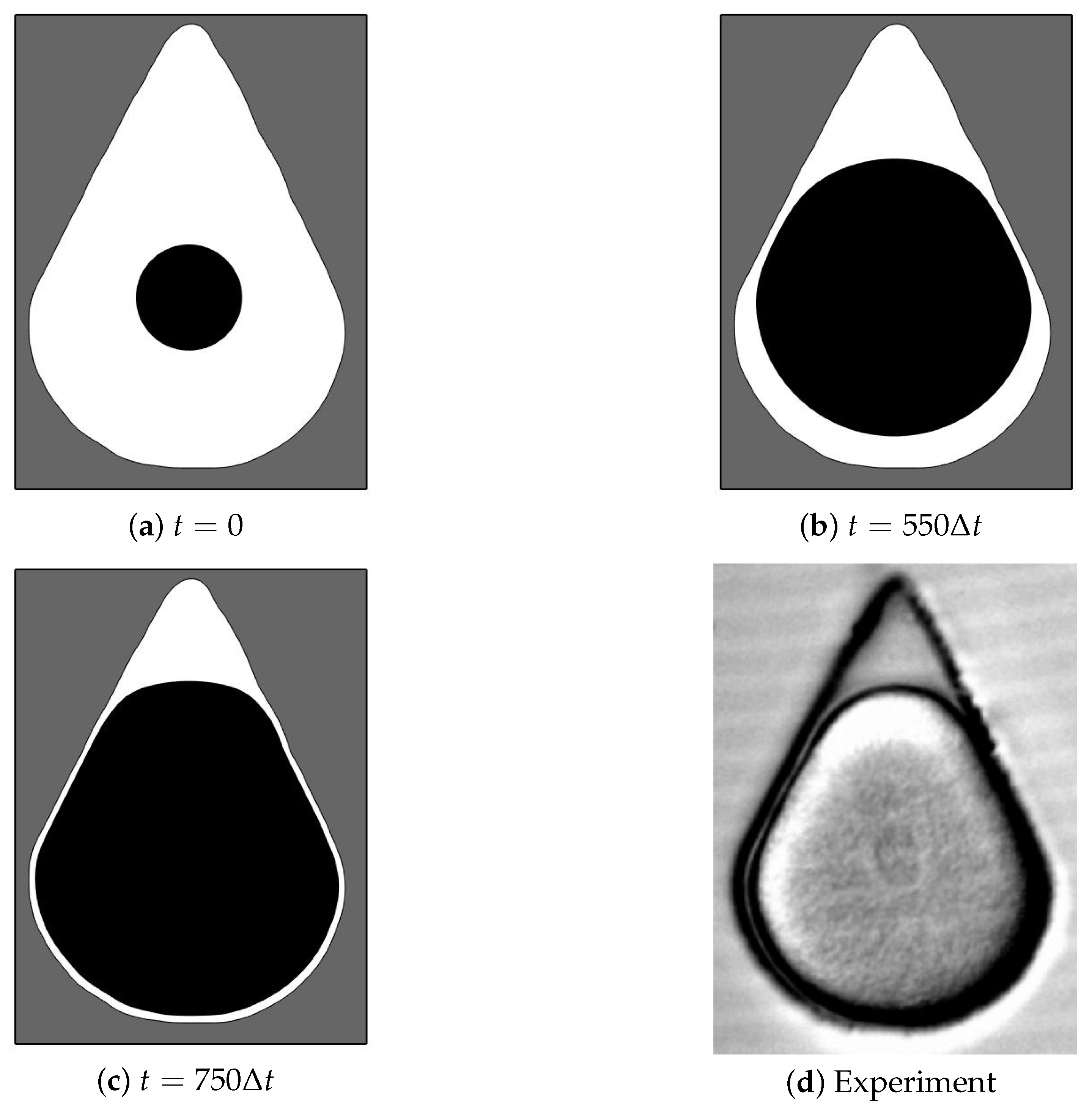
3.3. Cell Growth in a Complex Domain

In this section, we consider a growing cell inside a non-rectangular domain. To simulate cell growth, we set the time-dependent parameter $\beta \left(t\right)$ in Equation (2) as constant $\beta$. That is,

$$\begin{array}{c}\hfill \frac{\partial \varphi (\mathbf{x},t)}{\partial t}=-\frac{F^{\prime }\left(\varphi (\mathbf{x},t)\right)}{{ϵ}^2}+\Delta \varphi (\mathbf{x},t)+\beta \sqrt{F\left(\varphi \right(\mathbf{x},t\left)\right)},\mathbf{x}\in {\Omega }_{in},t>0,\end{array}$$

(30)

where ${\Omega }_{in}$ is a complex domain. Figure 5 illustrates the discrete complex domain ${\Omega }_{in}^h$ embedded in $\Omega$ and ${\Omega }_{out}^h=\Omega /{\Omega }_{in}^h$. The open and solid circles (∘, •) represent the grid points inside and outside the complex domain, respectively.

We present a numerical scheme for Equation (30) in a complex domain with the Dirichlet boundary condition, i.e., ${\varphi }_{ij}^n=-1$ for $(x_i,y_j)\in {\Omega }_{out}^h$. We solve Equation (30) only in ${\Omega }_{in}^h$ by using the operator splitting method (6)–(8). Here, we replace Equation (8) by

$$\begin{array}{c}\hfill \frac{{\varphi }_{ij}^{n+1}-{\varphi }_{ij}^{n+1,2}}{\Delta t}=\beta \sqrt{F\left({\varphi }_{ij}^{n+1,2}\right)}.\end{array}$$

(31)

Figure 6a–c shows the temporal evolutions of the initial disk in a complex domain which is star-shaped at $t=0,800\Delta t,$ and $1100\Delta t$. The shape of the domain is created with the image in Figure 6d. The initial condition on the embedding domain $\Omega =(0,1)\times (0,1)$ is defined by

$$\begin{array}{c}\hfill \varphi (x,y,0)=tanh\frac{0.15-\sqrt{{(x-0.43)}^2+{(y-0.5)}^2}}{\sqrt{2}ϵ}.\end{array}$$

Here, we use $N_x=N_y=125$, $h=1/124$, $\Delta t=0.1h^2$, $ϵ={ϵ}_{12}$, and $\beta =2h$ to make the cell grow.

In Figure 7a–c, we illustrate the temporal evolutions in a drop-shaped domain which we created with Figure 7d at $t=0,550\Delta t,$ and $750\Delta t$. We use $N_x=92$, $N_y=124$, $h=1/(N_x-1)$, $\Delta t=0.1h^2$, $ϵ={ϵ}_{12}$, and $\beta =2h$ to make the cell grow. The initial condition on the embedding domain $\Omega =(0,(N_x-1)h)\times (0,(N_y-1)h)$ is defined by

$$\begin{array}{c}\hfill \varphi (x,y,0)=tanh\frac{0.15-\sqrt{(x-0.5(N_x-1)h){)}^2+{(y-0.4(N_y-1)h)}^2}}{\sqrt{2}ϵ}.\end{array}$$

We can obtain a similar computational result with a much simpler proposed scheme compared to the previous complex method [29]. Moreover, while there is a restriction on the ratio of domain sizes when we use a multigrid method, we do not have that restriction in the proposed method.

4. Conclusions

We proposed the explicit hybrid numerical method for the nonlocal AC equation with isotropically symmetric interfacial energy in this paper. In general, an explicit time-stepping scheme is not suitable for solving large systems because it requires strong time step restrictions and this further causes a stability problem. Because the AC model is of the second order, however, this gives a rationale for solving such drawbacks. For example, the nonlocal AC equation can be applied to many fields by replacing the Cahn–Hillard equation which is a fourth-order equation [30]. The AC model does not take much time to evaluate numerical solutions; hence numerical solutions can be obtained at a relatively adequate time as depicted in Table 1 even though one uses the explicit hybrid scheme. Accordingly, robustness and accuracy can be also achieved simultaneously when a sufficiently small size of time step is applied. Numerical tests are presented to demonstrate the basic property of the nonlocal AC equation and usefulness of the proposed method. Moreover, we performed numerical experiments for the area-preserving mean curvature flow. There have been good agreements between the theoretical solutions and the computational results. Compared to the fully implicit scheme, the proposed method is more accurate with similar elapsed time though the implicit scheme is still suitable for long time simulation. In the last section, numerical simulations confirm that the proposed method is not affected by the shapes of domain. Considering that it is common to employ square grids when an implicit numerical scheme is used for complex domains, the proposed algorithm is much simpler and faster. This is the reason the proposed method is preferred over the existing methods, and there are some direct applications of it such as smoothing the surface with volume objects [31], direct computation in narrow band corresponding to surface [32], etc. Therefore, the proposed method can be used efficiently with little input cost and get accurate numerical solutions.

References

1. Stenger, F.; Voigt, A. Towards infinite tilings with symmetric boundaries. Symmetry 2019, 11, 444. [Google Scholar] [CrossRef] [Green Version]
2. Allen, S.M.; Cahn, J.W. A microscopic theory for antiphase boundary motion and its application to antiphase domain coarsening. Acta Metall. 1979, 27, 1085–1095. [Google Scholar] [CrossRef]
3. Broadbridge, P.; Triadis, D.; Gallage, D.; Cesana, P. Nonclassical symmetry solutions for fourth-order phase field reaction-diffusion. Symmtery 2018, 10, 72. [Google Scholar] [CrossRef] [Green Version]
4. Jeong, D.; Kim, J. An explicit hybrid finite difference scheme for the Allen–Cahn equation. J. Comput. Appl. Math. 2018, 340, 247–255. [Google Scholar] [CrossRef]
5. Lee, S.; Lee, D. The fractional Allen–Cahn equation with the sextic potential. Appl. Math. Comput. 2019, 351, 176–192. [Google Scholar] [CrossRef]
6. Li, C.; Huang, Y.; Yi, N. An unconditionally energy stable second order finite element method for solving the Allen–Cahn equation. J. Comput. Appl. Math. 2019, 353, 38–48. [Google Scholar] [CrossRef]
7. Lee, H.G.; Park, J.; Yoon, S.; Lee, C.; Kim, J. Mathematical model and numerical simulation for tissue growth on bioscaffolds. Appl. Sci. 2019, 9, 4058. [Google Scholar] [CrossRef] [Green Version]
8. Hu, X.; Li, Y.; Ji, H. A nodal finite element approximation of a phase field model for shape and topology optimization. Appl. Math. Comput. 2018, 339, 675–684. [Google Scholar] [CrossRef]
9. Sire, Y.; Valdinoci, E. Fractional Laplacian phase transitions and boundary reactions: A geometric inequality and a symmetry result. J. Funct. Anal. 2009, 256, 1842–1864. [Google Scholar] [CrossRef] [Green Version]
10. Brassel, M.; Bretin, E. A modified phase field approximation for mean curvature flow with conservation of the volume. Math. Methods Appl. Sci. 2011, 34, 1157–1180. [Google Scholar] [CrossRef]
11. Rubinstein, J.; Sternberg, P. Nonlocal reaction-diffusion equations and nucleation. IMA J. Appl. Math. 1992, 48, 249–264. [Google Scholar] [CrossRef]
12. Kim, J.; Lee, S.; Choi, Y. A conservative Allen–Cahn equation with a space-time dependent Lagrange multiplier. Int. J. Eng. Sci. 2014, 84, 11–17. [Google Scholar] [CrossRef]
13. Chai, Z.; Sun, D.; Wang, H.; Shi, B. A comparative study of local and nonlocal Allen–Cahn equations with mass conservation. Int. J. Heat Mass Transf. 2018, 122, 631–642. [Google Scholar] [CrossRef]
14. Zhang, J.; Chen, C.; Yang, X.; Chu, Y.; Xia, Z. Efficient, non-iterative, and second-order accurate numerical algorithms for the anisotropic Allen–Cahn Equation with precise nonlocal mass conservation. J. Comput. Appl. Math. 2020, 363, 444–463. [Google Scholar] [CrossRef]
15. Guan, Z.; Lowengrub, J.; Wang, C. Convergence analysis for second-order accurate schemes for the periodic nonlocal Allen–Cahn and Cahn–Hilliard equations. Math. Methods Appl. Sci. 2017, 40, 6836–6863. [Google Scholar] [CrossRef] [Green Version]
16. Du, Q.; Yang, J. Fast and accurate implementation of Fourier spectral approximations of nonlocal diffusion operators and its applications. J. Comput. Phys. 2017, 332, 118–134. [Google Scholar] [CrossRef] [Green Version]
17. Lee, H.G. High-order and mass conservative methods for the conservative Allen–Cahn equation. Comput. Math. Appl. 2016, 72, 620–631. [Google Scholar] [CrossRef]
18. Weng, Z.; Zhuang, Q. Numerical approximation of the conservative Allen–Cahn equation by operator splitting method. Math. Methods Appl. Sci. 2017, 40, 4462–4480. [Google Scholar] [CrossRef]
19. Zhai, S.; Weng, Z.; Feng, X. Fast explicit operator splitting method and time-step adaptivity for fractional non-local Allen–Cahn model. Appl. Math. Model. 2016, 40, 1315–1324. [Google Scholar] [CrossRef]
20. Ren, F.; Song, B.; Sukop, M.C.; Hu, H. Improved lattice Boltzmann modeling of binary flow based on the conservative Allen–Cahn equation. Phys. Rev. E 2016, 94, 023311. [Google Scholar] [CrossRef] [Green Version]
21. Aihara, S.; Takaki, T.; Takada, N. Multi-phase-field modeling using a conservative Allen–Cahn equation for multiphase flow. Comput. Fluids 2019, 178, 141–151. [Google Scholar] [CrossRef]
22. Joshi, V.; Jaiman, R.K. An adaptive variational procedure for the conservative and positivity preserving Allen–Cahn phase-field model. J. Comput. Phys. 2018, 366, 478–504. [Google Scholar] [CrossRef] [Green Version]
23. Li, Y.; Lee, H.G.; Jeong, D.; Kim, J. An unconditionally stable hybrid numerical method for solving the Allen–Cahn equation. Comput. Math. Appl. 2010, 60, 1591–1606. [Google Scholar] [CrossRef] [Green Version]
24. Kim, J. Phase-field models for multi-component fluid flows. Commun. Comput. Phys. 2012, 12, 613–661. [Google Scholar] [CrossRef]
25. Bronsard, L.; Stoth, B. Volume-preserving mean curvature flow as a limit of a nonlocal Ginzburg–Landau equation. SIAM J. Math. Anal. 1997, 28, 769–807. [Google Scholar] [CrossRef] [Green Version]
26. Kanagarajan, K.; Suresh, R. Runge–Kutta method for solving fuzzy differential equations under generalized differentiability. Comput. Appl. Math. 2018, 37, 1294–1305. [Google Scholar] [CrossRef]
27. Jeong, D.; Kim, J. Conservative Allen–Cahn–Navier–Stokes system for incompressible two-phase fluid flows. Comput. Fluids 2017, 156, 239–246. [Google Scholar] [CrossRef]
28. Minc, N.; Burgess, D.; Chang, F. Influence of cell geometry on division-plane positioning. Cell 2011, 144, 414–426. [Google Scholar] [CrossRef] [Green Version]
29. Li, Y.; Jeong, D.; Shin, J.; Kim, J. A conservative numerical method for the Cahn—Hilliard equation with Dirichlet boundary conditions in complex domains. Comput. Math. Appl. 2013, 65, 102–115. [Google Scholar] [CrossRef]
30. Yang, J.; Li, Y.; Lee, C.; Kim, J. Conservative Allen–Cahn equation with a nonstandard variable mobility. Acta Mech. 2020, 231, 561–576. [Google Scholar] [CrossRef]
31. Wang, J.; Li, Y.; Choi, Y.; Lee, C.; Kim, J. Fast and accurate smoothing method using a modified Allen—Cahn equation. Comput. Aided Des. 2020, 120, 102804. [Google Scholar] [CrossRef]
32. Kim, J.; Jeong, D.; Yang, S.D.; Choi, Y. A finite difference method for a conservative Allen–Cahn equation on non-flat surfaces. J. Comput. Phys. 2017, 334, 170–181. [Google Scholar] [CrossRef]
Figure 1. (a) Evolutions of the radii ( R 1 ( t ) , R 2 ( t ) , and R 3 ( t ) ) of three distinct disks at t = 0, 17,500 Δ t and 22,150 Δ t . (b) Comparison of the numerical solutions of three radii (star, circle, and diamond marks), the reference solution of three radii (solid line), and the reference solution of the average of R 1 ( t ) and R 3 ( t ) (dashed line).
Symmetry 12 01218 g001
Figure 2. (a) Evolutions of the radii ( R 1 ( t ) , R 2 ( t ) , and R 3 ( t ) ) of three distinct disks at t = 0, 19,000 Δ t and 22,500 Δ t . (b) Comparison of the numerical solutions of three radii (star, circle, and diamond marks), the reference solution of three radii (solid line), and the reference solution of the average of R 1 ( t ) and R 3 ( t ) (dashed line).
Symmetry 12 01218 g002
Figure 3. (a) Evolutions of the radii ( R 1 ( t ) , R 2 ( t ) , and R 3 ( t ) ) of three distinct disks with R 2 0 = 0.18 at t = 0, 13,000 Δ t , and 26,000 Δ t . (b) Comparison of the numerical solutions of three radii (star, circle, and diamond marks), the reference solution of three radii (solid line), and the reference solution of the average of R 1 ( t ) and R 3 ( t ) (dashed line).
Symmetry 12 01218 g003
Figure 4. (a) Evolutions of two disks with the explicit hybrid scheme at t = 0 (dotted line), 2000 Δ t (dashed line), and 4000 Δ t (solid line). (b) Evolution of two radii.
Symmetry 12 01218 g004
Figure 5. Discrete complex domain Ω i n h .
Symmetry 12 01218 g005
Figure 6. (ac) Evolutions of cell growth in a star-shaped domain. (d) Figure of the experiment in [28], which is reprinted with permission from Minc et al., Cell, 144, 414–426 (2011), ©2011, Elsevier.
Symmetry 12 01218 g006
Figure 7. (ac) Evolutions of cell growth in a drop-shaped domain. (d) Figure of the experiment in [28], which is reprinted with permission from Minc et al., Cell, 144, 414–426 (2011), ©2011, Elsevier.
Symmetry 12 01218 g007