Imbalanced Data Fault Diagnosis Based on an Evolutionary Online Sequential Extreme Learning Machine

Abstract
1. Introduction
2. ABC-OSELM
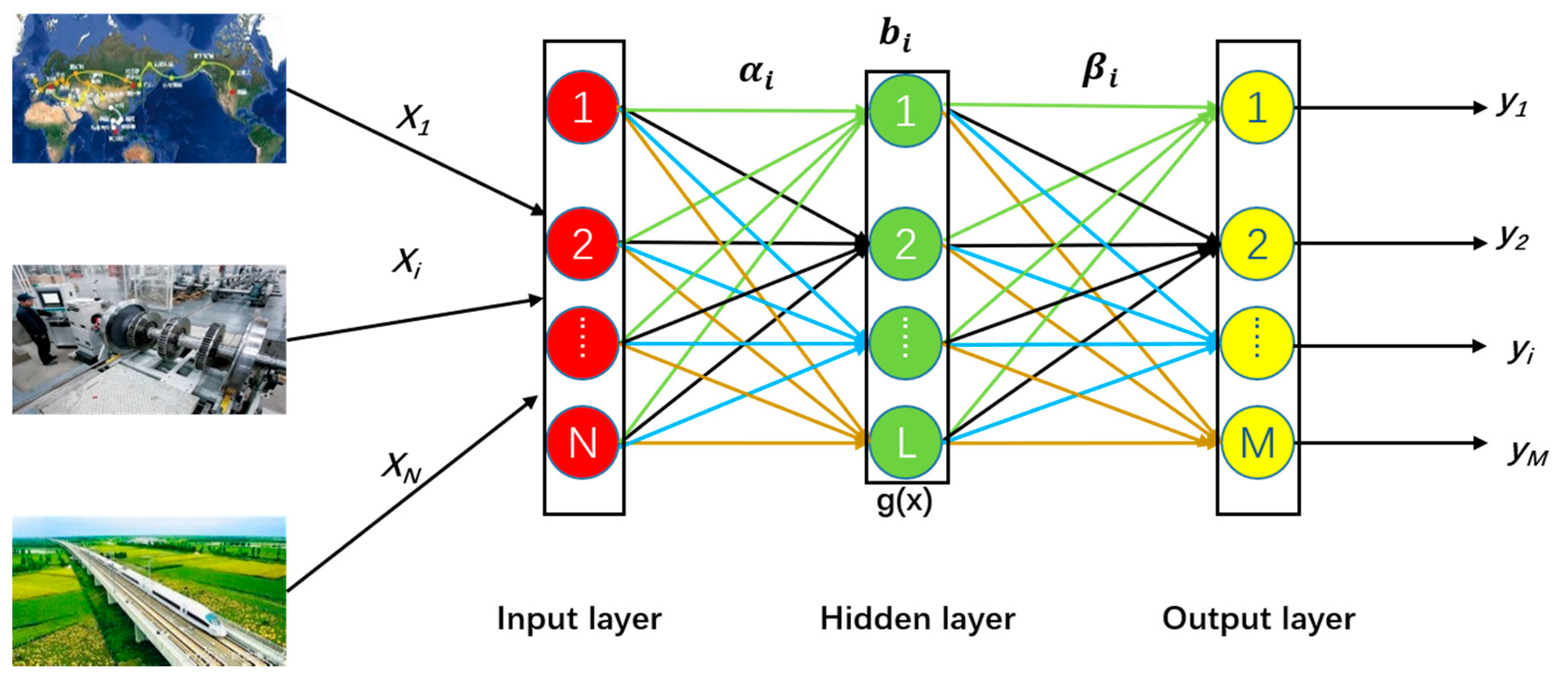
2.1. OS-ELM
2.1.1. Initialization
2.1.2. Online Sequential Learning
2.2. Artificial Bee Colony
2.2.1. Initialization
2.2.2. Optimization
Employed Bees
- The employed bees should exploit nectar sources and find out the amounts of nectar in food sources. Every one of the nectar sources represents a feasible solution to the problem, and the nectar amounts represent the fitness value of the solution.
- The employed bees then locate a new candidate source away from the previous one and compare the nectar amounts of the two, then choose the richer one. The new candidate source location is generated from its predecessor using Equation (16):where denotes the new location, while denotes the previous location and is an arbitrary source location in the neighborhood of the previous location, with the indices , where marks the colony scale, and where marks the dimensions of the problem. is a random number following a uniform distribution within .
Onlooker Bees
Scout Bees
2.3. ABC-OSELM
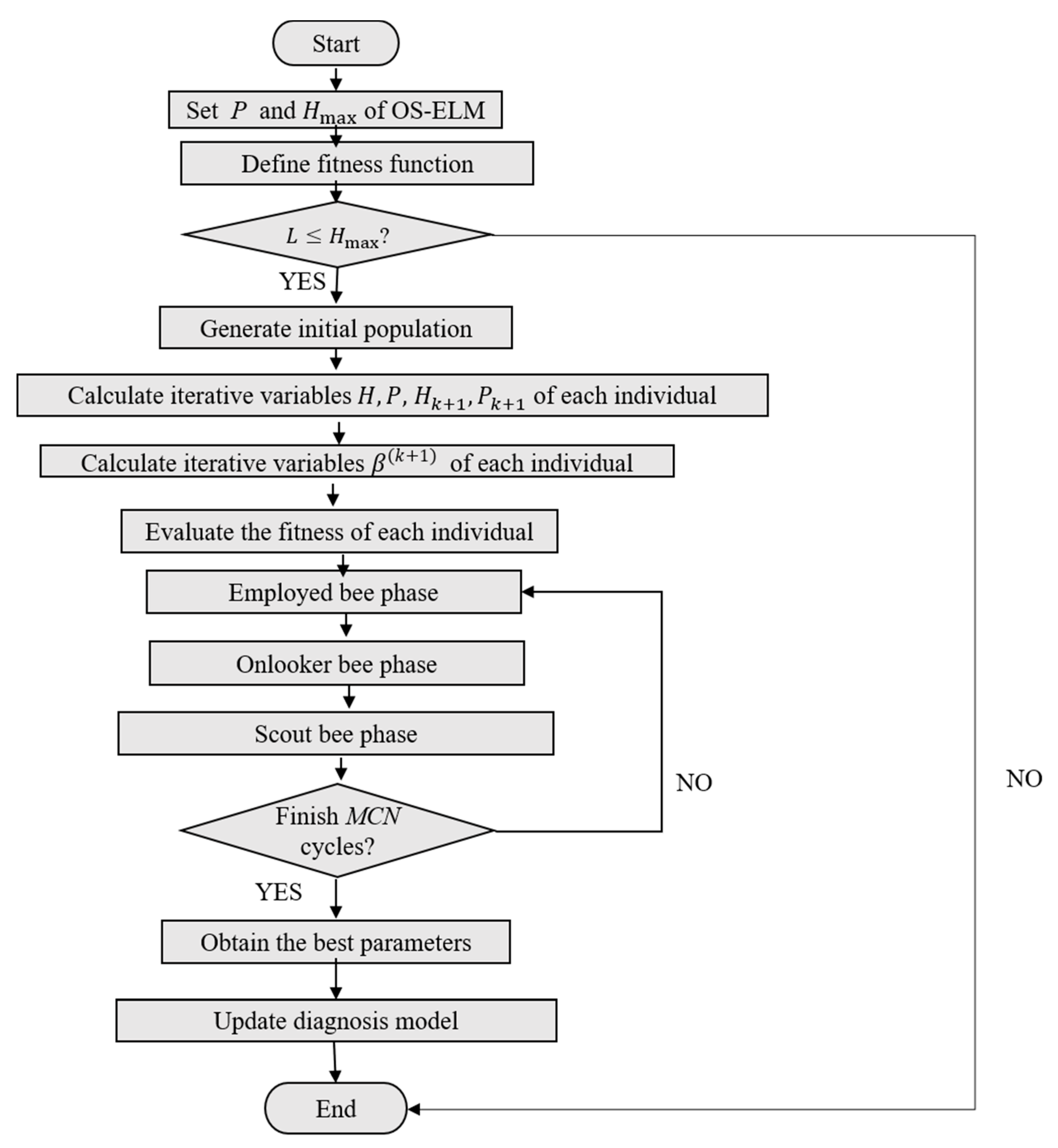
- Set the chunk size P and the maximum hidden layer nodes number .
- Generate the initial population randomly. Each initial solution vector contains input weights, a hidden layer bias, and the initialization parameters, i.e., MCN, limit, and upper/lower bounds of the search space need to be established depending on the number of hidden layer nodes:where n and m are the numbers of nodes in the input layer and the hidden layer, respectively.
- For each individual, calculate the output weight matrix
- Calculate the fitness value of each solution vector.
- Repeat the employed bees’, onlooker bees’, and scout bees’ search processes until MCN cycles are completed.
- Record the best parameters and update the diagnosis model.
3. Imbalanced Axle Box Bearing Fault Diagnosis Based on the Evolutionary OS-ELM
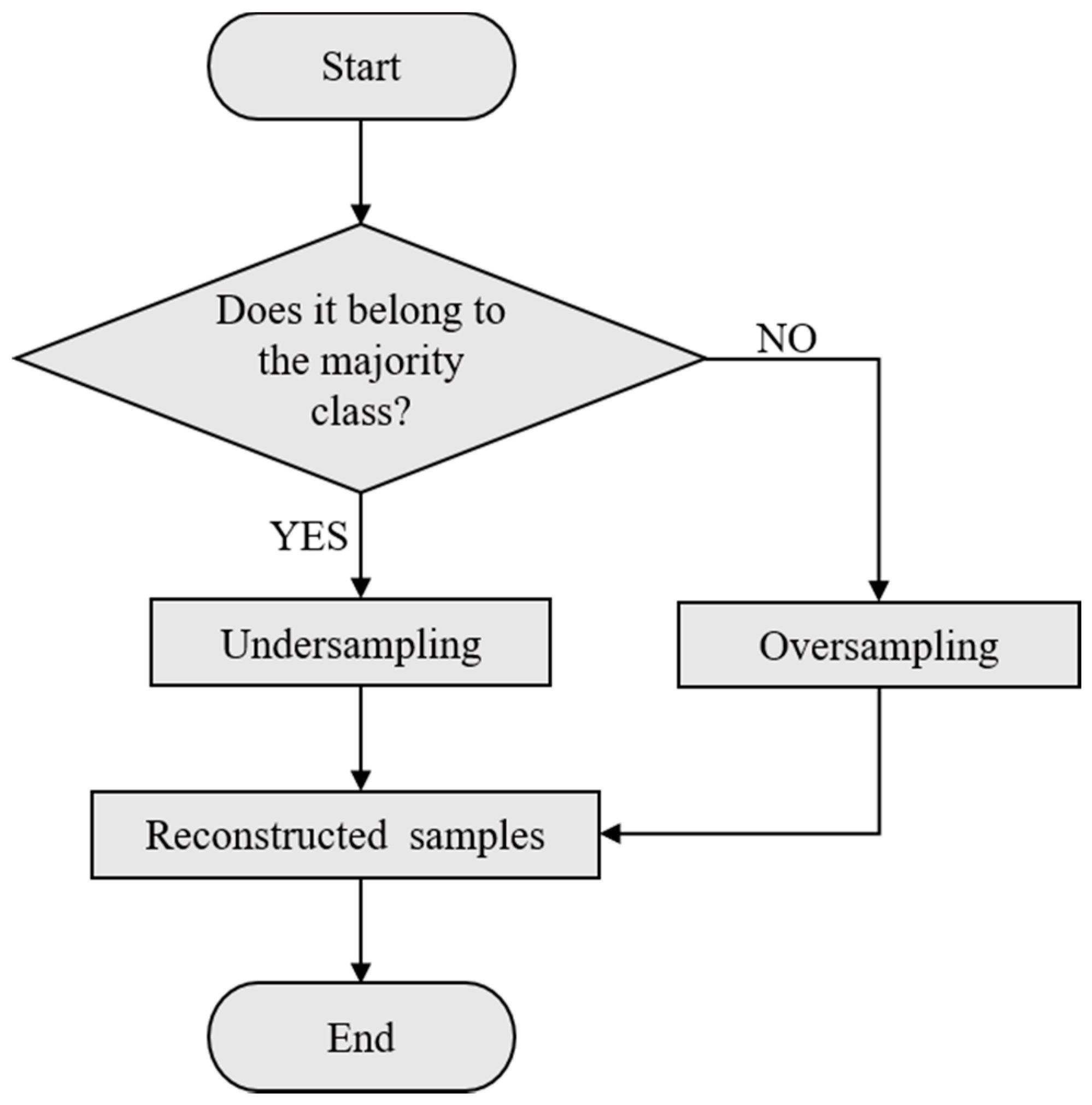
3.1. Imbalanced Data Mixed Resampling
- The sample set D made up of historical monitored data of high-speed EMU axle box bearings is classified according to the sample’s properties. The minority class sample set is defined as S. The majority class sample set is defined as M.
- Using the resampling empirical Equation (20) proposed in Porwik et al. [18] for the imbalanced data dichotomy, the resampling scales are set as follows:where is the oversampling scale for the minimum class () and is the undersampling scale for the maximum class (). R denotes the ratio of the number of the minority class samples to the number of majority class samples.
- Oversampling of the minority class samples using K-means SMOTE is based on the clustering distribution. In the beginning, filter the targeted clusters and save the ones that are numerically dominant within the minority class samples by generating k clusters using K-means algorithms. Then, distribute the quantity of the clustering samples while preferring the sparse groups. To prevent undesirable noise, only data relating to key indicators are oversampled, while the rest are kept in their original form to highlight the more informative and significant indicators. Finally, new samples are generated in each selected cluster with SMOTE and added to the minority class sample set M.
- Undersample the majority class samples in non-boundary domains with the method based on the Euclidean distance. First, locate the center of the majority class sample set M by calculating the distances between all the sample points to the center and ranking them in order. From the furthest sample point to the center, delete samples in M according to the undersampling magnification until M is quantitatively balanced with the minority class samples. This approach identifies the classification boundary and leaves out the insignificant and distant samples from the classification boundary in the majority class, which ensures that the training dataset is composed of safe samples.
- Derive a new sample set from the updated minority class samples and majority class samples.
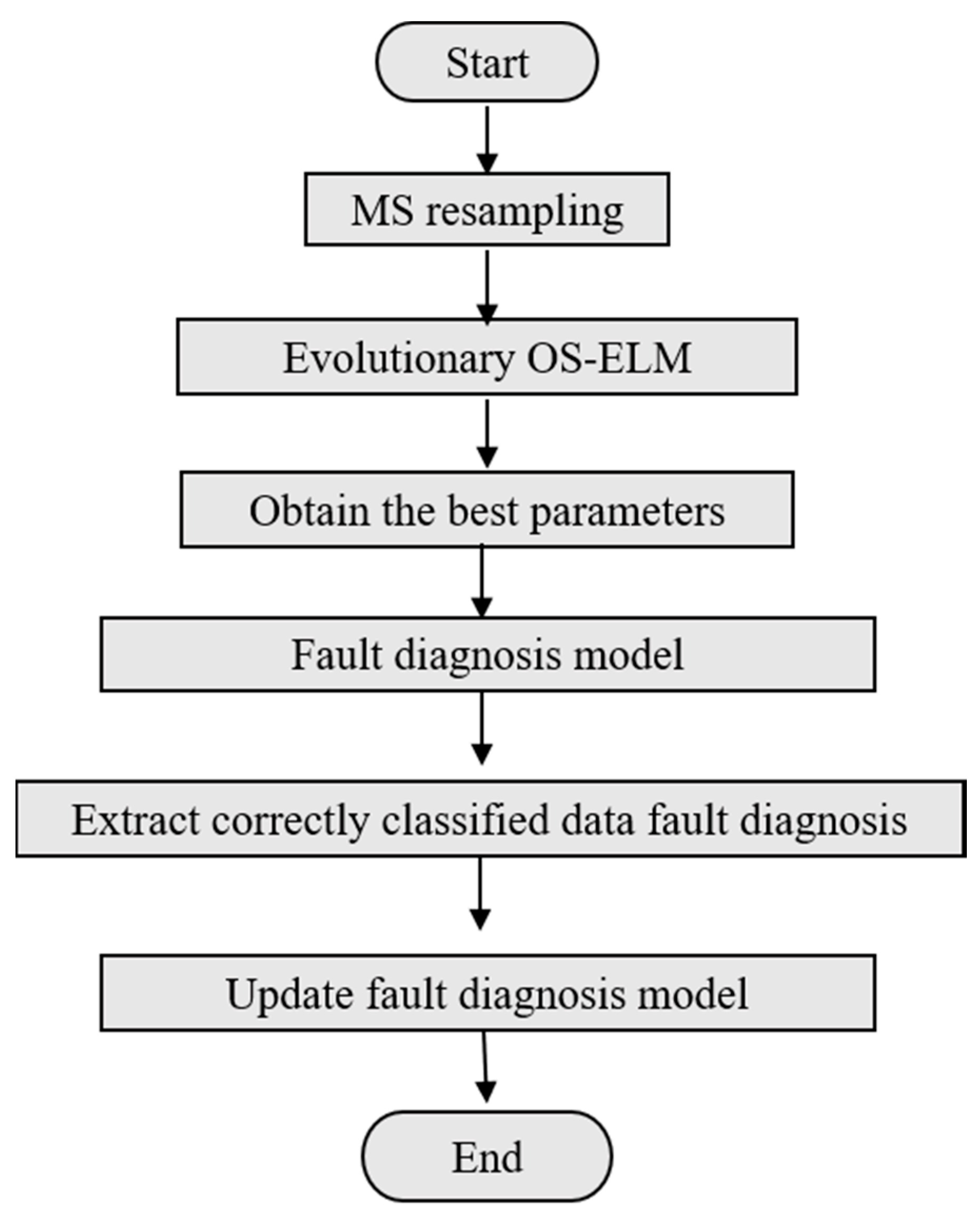
3.2. Diagnosis Process
- Resample the imbalanced data by extracting the required high-speed EMU axle box bearing data and dividing them into minority class samples and majority class samples. Determine the resampling scale of the imbalanced data and reconstruct the training dataset with mixed resampling methods to acquire new training samples.
- Use the evolutionary OS-ELM algorithm to search for the global optimum sets of the input weights and hidden layer bias under different numbers of hidden layer nodes for the OS-ELM, as discussed in Section 2.
- Report the best combination of variables and note down the optimized input weights and hidden layer bias with the number of hidden layer nodes.
- Establish the optimized diagnosis model.
- Update the fault diagnosis model using the accurately diagnosed historical data as the online sequential sample. These online sequential samples are then reconstructed to a balanced distribution. Compute and , then update the diagnosis model using the OS-ELM. Repeat step (5) and optimize the high-speed EMU axle box bearing fault diagnosis model through adaptive learning.
4. Experiments and Analysis
4.1. Dataset
4.2. Assessment Criteria
4.3. Analysis
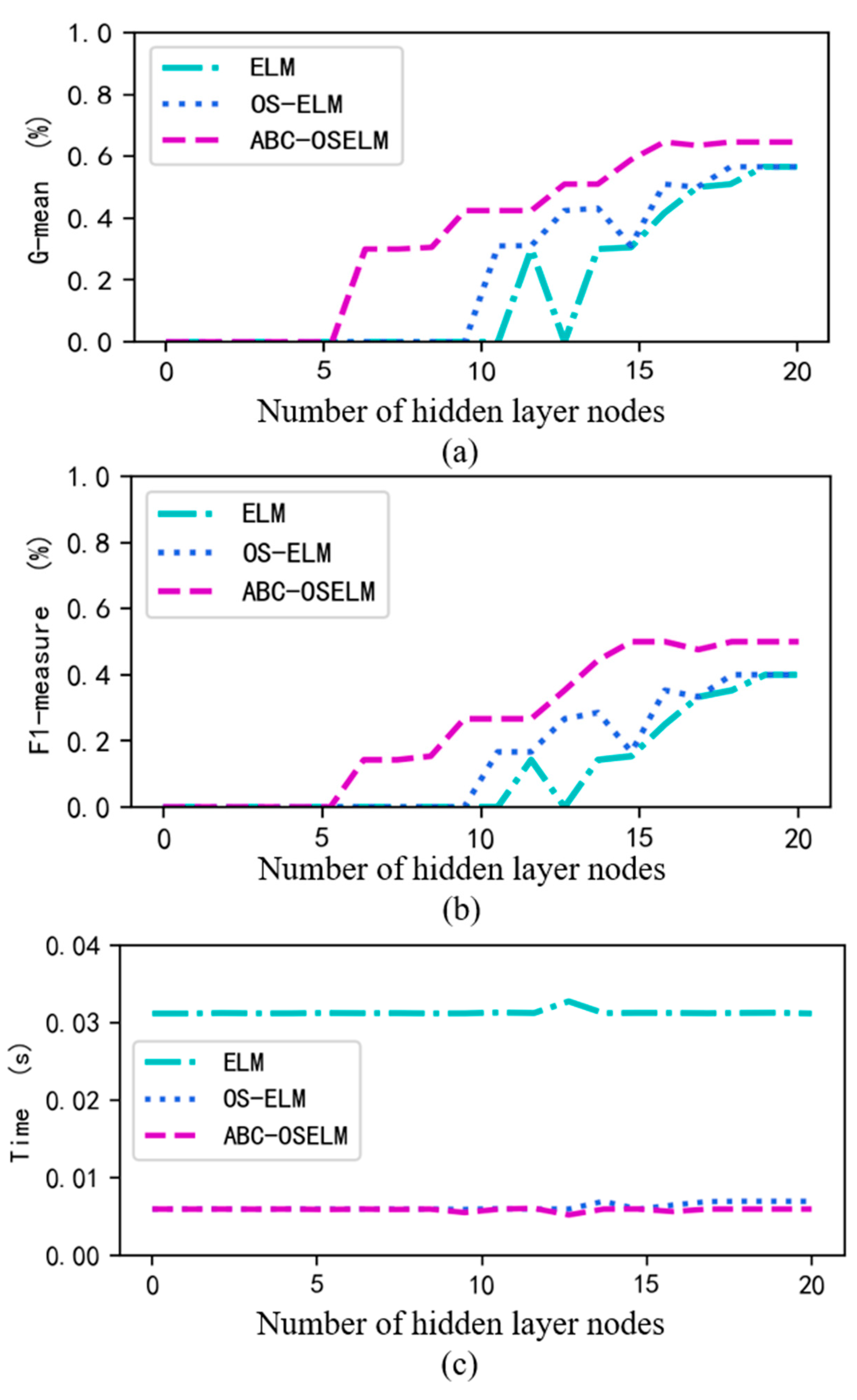
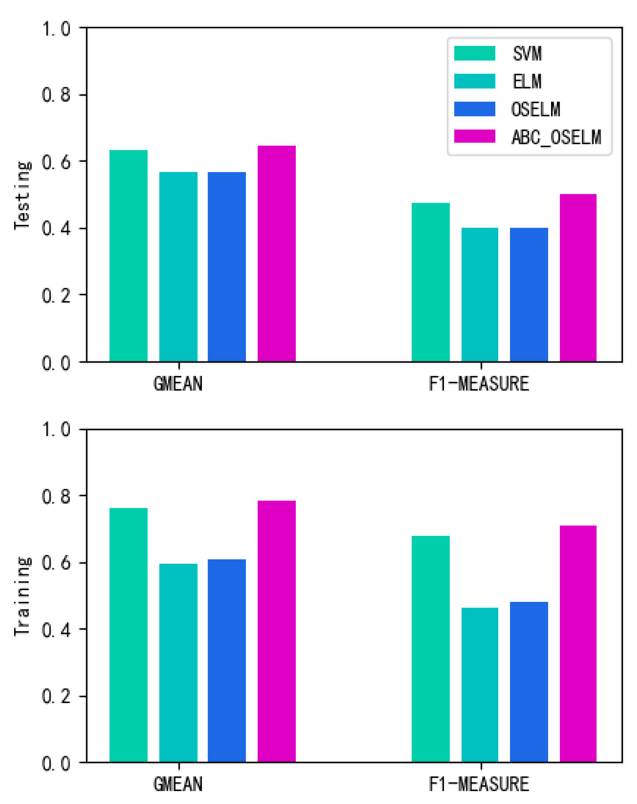
4.3.1. Algorithm Efficiency Analysis on the Original Dataset
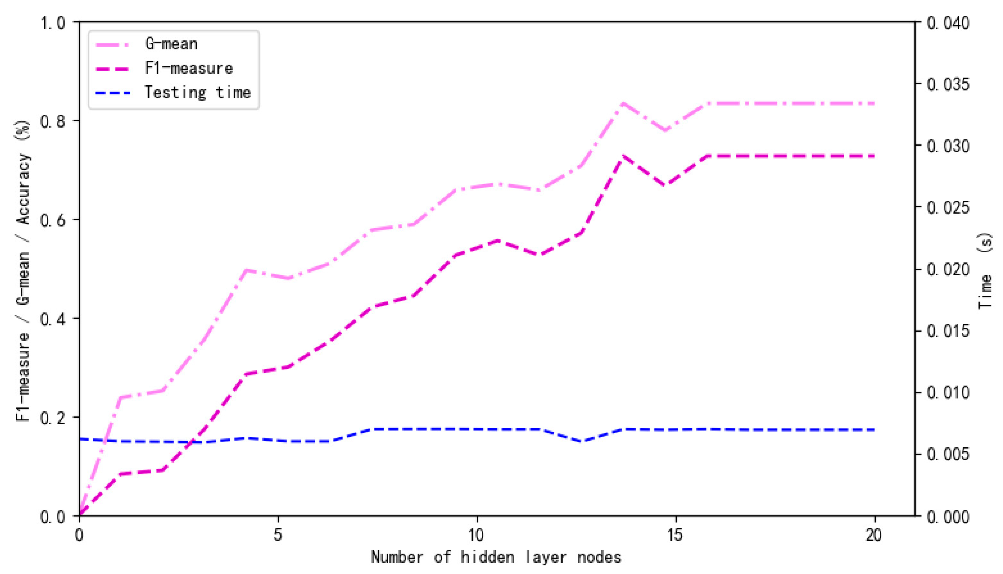
4.3.2. Algorithm Analysis on the Mixed Resampling Dataset
5. Conclusions
Author Contributions
Funding
Conflicts of Interest
References
- Zhao, B.; Yuan, Q.; Zhang, H. A Real-Time Fault Early Warning Method for a High-Speed EMU Axle Box Bearing. Sensors 2020, 20, 823. [Google Scholar]
- Qin, N.; Jin, W.; Huang, J.; Li, Z.M. Ensemble empirical mode decomposition and fuzzy entropy in fault feature analysis for high-speed train bogie. Control Theory Appl. 2014, 31, 1246–1251. [Google Scholar]
- Huang, X.W.; Liu, C.M.; Feng, C.; Wang, X.; Yu, F. Failure diagnosis system for CRH3 electrical multiple unit. Comput. Integr. Manuf. Syst. 2010, 16, 2311–2318. [Google Scholar]
- Zhou, B.; Xu, W. Improved parallel frequent pattern growth algorithm in EMU’s fault diagnosis knowledge mining. Comput. Integr. Manuf. Syst. 2016, 22, 2450–2457. [Google Scholar]
- Li, P.; Zheng, J. Fault Diagnosis Based on Multichannel Vibration Signal for Port Machine Trolley Wheel Bearings. Bearing 2007, 9, 35–38. [Google Scholar]
- Liu, J.; Zhao, Z.; Zhang, G.; Wang, G.M.; Meng, S.; Ren, G. Research on fault diagnosis method for bogie bearings of Metro vehicle. J. China Railw. Soc. 2015, 37, 30–36. [Google Scholar]
- Feng, H.; Yao, B.; Gao, Y.; Wang, H.; Feng, J. Imbalanced data processing algorithm based on boundary mixed sampling. Control Dec. 2017, 10, 1831–1836. [Google Scholar]
- Wuchu, T.; Minjie, W.; Guangdong, C.; Yuchao, S.; Li, X. Analysis on temperature distribution of failure axle box bearings of high-speed train. J. China Railw. Soc. 2016, 38, 50–56. [Google Scholar]
- Yin, H.X.; Wang, K.; Zhang, T.Z. Fault Prediction Based on PSO—BP Neural Network About Wheel and Axle Box of Bogie in Urban Rail Train. Complex Syst. Complex. Sci. 2015, 12, 97–103. [Google Scholar]
- Liu, J.; Zhao, Z.; Ren, G. An intelligent fault diagnosis method for bogie bearings of train based on wavelet packet decomposition and EEMD. J. China Railw. Soc. 2015, 37, 41–46. [Google Scholar]
- Liang, N.Y.; Huang, G.B.; Saratchandran, P.; Sundararajan, N. A Fast and Accurate Online Sequential Learning Algorithm for Feedforward Networks. IEEE Trans. Neural Netw. 2006, 17, 1411–1422. [Google Scholar] [CrossRef] [PubMed]
- Jia, P.; Wu, Q.; Li, L. Objective-driven dynamic dispatching rule for semiconductor wafer fabrication facilities. Comput. Integr. Manuf. Syst. 2014, 20, 2808–2813. [Google Scholar]
- Hussain, T.; Siniscalchi, S.M.; Lee, C.C.; Wang, S.S.; Tsao, Y.; Liao, W.H. Experimental study on extreme learning machine applications for speech enhancement. IEEE Access 2017, 5, 25542–25554. [Google Scholar] [CrossRef]
- Fan, J.M.; Fan, J.P.; Liu, F. A Novel Machine Learning Method Based Approach for Li-Ion Battery Prognostic and Health Management. IEEE Access 2019, 7, 160043–160061. [Google Scholar] [CrossRef]
- Lu, S.; Lu, Z.; Yang, J.; Yang, M.; Wang, S. A pathological brain detection system based on kernel based ELM. Multimed. Tools Appl. 2018, 77, 3715–3728. [Google Scholar] [CrossRef]
- Zhu, Q.Y.; Qin, A.K.; Suganthan, P.N.; Huang, G.B. Evolutionary extreme learning machine. Pattern Recognit. 2005, 38, 1759–1763. [Google Scholar] [CrossRef]
- Arar, Ö.F.; Ayan, K. Software defect prediction using cost-sensitive neural network. Appl. Soft Comput. 2015, 33, 263–277. [Google Scholar] [CrossRef]
- Porwik, P.; Orczyk, T.; Lewandowski, M.; Cholewa, M. Feature projection k-NN classifier model for imbalanced and incomplete medical data. Biocybern. Biomed. Eng. 2016, 36, 644–656. [Google Scholar] [CrossRef]
- Fiore, U.; De Santis, A.; Perla, F.; Zanetti, P.; Palmieri, F. Francesca Perla Using generative adversarial networks for improving classification effectiveness in credit card fraud detection. Inf. Sci. 2019, 479, 448–455. [Google Scholar] [CrossRef]
- Qian, Y.; Liang, Y.; Li, M.; Feng, G.; Shi, X. A resampling ensemble algorithm for classification of imbalance problems. Neurocomputing 2014, 143, 57–67. [Google Scholar] [CrossRef]
- Wang, J.; Xu, Z.; Che, Y. Power Quality Disturbance Classification Based on DWT and Multilayer Perceptron Extreme Learning Machine. Appl. Sci. 2019, 9, 2315. [Google Scholar] [CrossRef]
- Gu, Y.; Zeng, L.; Qiu, G. Bearing Fault Diagnosis with Varying Conditions using Angular Domain Resampling Technology, SDP and DCNN. Measurement 2020, 156, 10761. [Google Scholar] [CrossRef]
- Piri, S.; Delen, D.; Liu, T. A synthetic informative minority over-sampling (SIMO) algorithm leveraging support vector machine to enhance learning from imbalanced datasets. Decis. Support Syst. 2018, 106, 15–29. [Google Scholar] [CrossRef]
- García, V.; Sánchez, J.S.; Mollineda, R.A. On the effectiveness of preprocessing methods when dealing with different levels of class imbalance. Knowl. Based Syst. 2012, 25, 13–21. [Google Scholar] [CrossRef]
- Xiong, B.; Wang, G.; Deng, W. Under-Sampling method based on sample weight for imbalanced data. J. Comput. Res. Dev. 2016, 53, 2613–2622. [Google Scholar]
- Gu, X.; Jiang, Y.; Wang, S. Zero-order TSK-type fuzzy system for imbalanced data classification. Acta Autom. Sin. 2017, 43, 1773–1788. [Google Scholar]
- Ju, Z.; Cao, J.; Gu, H. A fuzzy support vector machine algorithm for imbalanced data classification. J. Dalian Univ. Technol. 2016, 56, 252–531. [Google Scholar]
- Huang, G.B.; Zhou, H.; Ding, X.; Zhang, R. Extreme learning machine for regression and multiclass classification. IEEE Trans. Syst. 2012, 42, 513–529. [Google Scholar]
- Karaboga, D.; Basturk, B. A powerful and efficient algorithm for numerical function optimization: Artificial bee colony (ABC) algorithm. J. Glob. Optim. 2007, 39, 459–471. [Google Scholar] [CrossRef]


| No. | Property |
|---|---|
| 1 | Environment temperature |
| 2 | Running speed |
| 3 | Channel 1 temperature |
| 4 | Channel 2 temperature |
| 5 | Temperature of the coaxial bearings |
| 6 | Temperature of the same-sided bearings |
| 7 | Preorder temperature |
| 8 | Mile |
| 9 | Acceleration |
| 10 | Load |
| Predicted Positive Sample | Predicted Negative Sample | |
|---|---|---|
| Actual positive sample | TP | FN |
| Actual negative sample | FP | TN |
| Evaluation Metrics | SVM 1 | ELM | OS-ELM | ABC-OSELM |
|---|---|---|---|---|
| Testing time | 0.582 | 0.031 | 0.007 | 0.006 |
| Testing G-mean | 0.633 | 0.566 | 0.566 | 0.646 |
| Testing F1-measure | 0.476 | 0.4 | 0.4 | 0.5 |
| Training G-mean | 0.762 | 0.594 | 0.607 | 0.781 |
| Training F1-measure | 0.679 | 0.464 | 0.48 | 0.708 |
| Optimum node | / | 19 | 18 | 15 |
| Evaluation Metrics | SVM 1 | ELM | OS-ELM | ABC-OSELM |
|---|---|---|---|---|
| Resampling dataset | 0.779 | 0.721 | 0.764 | 0.833 |
| Original dataset | 0.633 | 0.566 | 0.566 | 0.646 |
| Evaluation Metrics | SVM 1 | ELM | OS-ELM | ABC-OSELM |
|---|---|---|---|---|
| Resampling dataset | 0.667 | 0.6 | 0.636 | 0.727 |
| Original dataset | 0.476 | 0.4 | 0.4 | 0.5 |
© 2020 by the authors. Licensee MDPI, Basel, Switzerland. This article is an open access article distributed under the terms and conditions of the Creative Commons Attribution (CC BY) license (http://creativecommons.org/licenses/by/4.0/).
Share and Cite
Hao, W.; Liu, F. Imbalanced Data Fault Diagnosis Based on an Evolutionary Online Sequential Extreme Learning Machine. Symmetry 2020, 12, 1204. https://doi.org/10.3390/sym12081204
Hao W, Liu F. Imbalanced Data Fault Diagnosis Based on an Evolutionary Online Sequential Extreme Learning Machine. Symmetry. 2020; 12(8):1204. https://doi.org/10.3390/sym12081204
Chicago/Turabian StyleHao, Wei, and Feng Liu. 2020. "Imbalanced Data Fault Diagnosis Based on an Evolutionary Online Sequential Extreme Learning Machine" Symmetry 12, no. 8: 1204. https://doi.org/10.3390/sym12081204
APA StyleHao, W., & Liu, F. (2020). Imbalanced Data Fault Diagnosis Based on an Evolutionary Online Sequential Extreme Learning Machine. Symmetry, 12(8), 1204. https://doi.org/10.3390/sym12081204